Bird breeding Avian Data:
Bayesian Statistical Updating Prediction for
the Size of Closed Population on the Species
Richness Model Using Generalized Binomial
Model with New Mixture Unit Interval Type
Prior for Animal Ecology
Jamal A. Al-Saleh
1, and Satish K. Agarwal
21
Department of Statistics and Operation Research, Faculty of Science, Kuwait University, P.O. Box 5969, Safat, Kuwait
2
Department of Mathematics, College of Science, University of Bahrain, P.O. Box 32038, Bahrain
Abstract In this article a new way of statistical updating prediction and measuring behavior in the field of animal population dynamics and ecological data science is studied and examined on the species richness model. To estimate the size of closed population, with individual heterogeneity in detection probability, we have introduced and used generalized binomial model with five parameters GBM(n,p,π,ρ,τ) [[1] Al-Saleh at el. (2016)], as an alternative model to the standard Binomial model SBM(n,p). The generalized model is developed by introducing new parameters called indicator parameters. The main advantage of an indicator parameter, is that, it will equip the new generalized model accession, more approaches, and options in statistical estimation for close fitting and measuring behavior of the data. To help with the examination of the data more precisely, we also consider a new mixture unit interval type prior on (0,1) with two parameters UITP(α,β), as an alternative model to the uniform prior on (0,1). To be a contrivance, and intermediary updating prediction model to exiting model [[2] Royle and Dorazio (2008), Chapter 6], and reproduce more effective, generalized, and propagated model of particular importance for species richness populations, using capture–recapture model. The estimate of the total population size could be affected by the selection of the model suggested to fit the data. Therefore, we propose an expanded, generalized, and extended model with the advantage that the model parameters can be estimated using Bayesian methodology which serves as a subtle resource for model identification and classification. An illustration is provided using species richness model with the application to bird breeding survey (BBS) data set. The generalized posterior summaries using Markov Chain Monte Carlo (MCMC) Gibbs sampling approach, are presented for the new models. The study of the parameters of the new models would help the users to have more clarity and understanding about the role of the existing model. It is found that proposed new models is more resilience, litheness, and is fully adaptive to the available data and gives animal ecologist another option for modelling the data.
Keywords generalized species richness model, Bayesian data analysis, generalized binomial distribution, unit interval type prior
I. INTRODUCTION
In this article we will address the above proposition by introducing an efficient statistical estimation process, and procedure, with a computational updating prediction techniques for the first time in animal population ecology data science. It is done by proposing a new generalized Binomial statistical model, with new mixture unit interval type prior for species richness model for estimating the size of a closed population with individual heterogeneity in detection probability. With this generalization setting in mind, we can find proper and suitable solutions for the data.
Generally, problems involving new generalized and extended statistical models based prediction, are well suited for the Bayesian methodology [see [5] King and Brooks (2001), [6] Royle al et. (2007), [1] Al-Saleh at el. (2016), [4] Al-Saleh and Agarwal (2017), and [7] Limaa al et. (2018)]. The motivation of this work is to explore these new generalized statistical models which can be used to provide a righteous, veracious, and adequate fit for the real data, than the usage of standard models. The Markov Chain Monte Carlo (MCMC) Gibbs sampling methods are used to simulate direct draws from the new generalized statistical model of interest. In section 2, we have proposed and studied new Bayesian approach for modelling species richness model, estimating the size of closed population with individual heterogeneity. In section 3, we have developed the generalized procedure to estimate the parameters of new models using Bayesian methodology. The Bayesian estimates of the parameters are obtained using Markov Chain Monte Carlo (MCMC) simulation technique based on the assumption that the new priors are independent, The generalized posterior analysis is performed and estimated. We have examine the issue of model compatibility using predictive results. A real data set of bird breeding survey (BBS) are analysed for illustrating the application and the proposed Bayesian approach.
II. THE MODEL
To establish and promote an efficient statistical estimation process, and procedure, for the problem of estimating the size of closed population. We first, introduce the five parameters generalized binomial model GBM(n,p,π,ρ,τ) [see [1] Al-Saleh at el. (2016)] with the following probability function
(2.1) f(y) = , π> 0, ρ 0, τ 0. y=0,1,…,n.
The model in equation (2.1) is developed by introducing three more parameters called indicator parameters. The main advantage of an indicator parameter is to give the generalized binomial model accession, more approaches, and options for fitting the data. When π=1, ρ=1, and τ=0, model (2.1) is reduced to standard binomial model [i.e., GBM(n,p,1,1,0) SBM(n,p)]. Also, to help with the examination of the data more precisely, we introduce new mixture unit interval type prior UITP(α,β) on (0,1) with two parameters > 0, β > 0, and its pdf is given by,
(2.2) f(x) = , , > 0, β > 0.
The distribution function of model (2.2) is F(x) ,
When =0, and β=1, the model (2.2) reduces to standard uniform model [UITP(0,1)= SUM(0,1)]. In some particular cases the parameters α, and β of model (2.2) can be seen as providing not only an extra flexibility to the probability function, but also helps to express probability distribution as an exact form of mixture of probability distributions under certain conditions.
procedure and data analysis study here follows that of [[2] Royle and Dorazio (2008), Chapter 6]. The specific data set consists of observed detections for n1 = 71 bird in a Breeding Bird Survey study in Maryland. There
were k=50 samples of the population. In this study we deal with unknown N by data augmentation, therefore we introduce zero readings, = 0,...,yM = 0, and a set of implicit variables zi, i= 1,2,...,M with zi have a standard
Bernoulli model. If zi= 1, then element i of the list blend with a member of the population of size N, and if zi=0, it is an excess 0 relative to the binomial model. M is set arbitrarily large. It can be motivated as the upper limit of a discrete uniform type prior for N. That is, N ~ DiscreetUniform(0,M). The population size parameter is N= . In the following data analysis, we have augmented the data set with 250 yi = 0 subjects [see Table A].
(i) Model I: Standard Binomial model with uniform prior [see [2] Royle and Dorazio (2008), Chapter 6]
(1) zi ~ GBM(1,psi,1,1,0) # Bernolli
(2) y
i ~ GBM(k,zi*pi,1,1,0) # Binomial
(3) logit(pi) ~ Normal(mu, tau) for i = 1, 2, ...., M
Prior distributions are:
(1) psi~SUM(0,1)
(2) mu~Norm(0,0.001)
(3) tau~Gamma(0.001, 0.001); sigma=
(ii) Model II: Standard Binomial model with mixture unit interval prior
(1) zi~GBM(1,psi,1,1,0) # Bernolli (2) yi~GBM(k,zi*pi,1,1,0) # Binomial (3) logit(pi)~Normal(mu,tau) for i = 1, 2, ...., M
Prior distributions are:
(1) psi ~ UITP(α,β) # Mixture Unit Interval Prior
(2) mu ~ Normal(0,0.001)
(3) tau ~ Gamma(0.001,0.001) ; sigma=
Hyper-Prior distributions are:
(1) α ~ Gamma(1.00,1.00)
(2) β ~ Gamma(1.00,1.00)
(iii) Model III: Generalized Binomial model with mixture unit interval prior
(1) zi ~ GBM(1,psi,1,1,0) # Bernolli
(2) yi ~ GBM(K,zi*pi,π,ρ,τ) # Generalized Binomial (3) logit(pi)~Normal(mu,tau) for i = 1, 2, ...., M
Prior distributions are:
(1) psi ~ UITP(α,β) # Mixture Unit Interval Prior
(2) mu ~ Norm(0,0.001)
(3) tau ~ Gamma(0.001,0.001); sigma=
(4) π ~ Gamma(1.00,1.00)
(5) ρ ~ Gamma(1.00,1.00)
(6) τ ~ Gamma(1.00,1.00)
Hyper-Prior distributions are:
(1) α ~ Gamma(1.00,1.00)
III. BAYESIAN UPDATING PREDICTION DATA ANALYSIS
A realistic Bayesian model for the bird breading survey data is to suggest a hierarchical model. A Markov Chain Monte Carlo (MCMC) Gibbs sampling approach implemented in using OPENBUGS@ computer software can give an analysis of estimates of each parameter. A burn in of 1000 updates followed by a further 100k updates is implemented. The table 3.1, represent the estimates for model I, the table 3.2, represent the estimates for model II, where the table 3.3, represent the estimates for model III, along with standard deviation, mean and MC error.
Table 3.1 Bayesian summary of estimates for model I
Mean SD MC error 2.5% Median 97.5%
N 88.92 10.57 0.7905 75.0 87.0 118.0
mu -2.658 0.4078 0.03107 -3.678 -2.595 -2.046 psi 0.2783 0.04101 0.002505 0.2127 0.2744 0.3751 Sigma 1.649 0.2793 0.02167 1.188 1.628 2.287
Table 3.2 Bayesian summary of estimates for model II
Mean SD MC error 2.5% Median 97.5%
N 90.82 11.82 0.9928 76.0 88.0 122.0
α
1.069 1.112 0.0216 0.02423 0.7092 4.181β
0.7629 0.8244 0.01668 0.009912 0.4965 3.032 mu -2.736 0.4404 0.03818 -3.82 -2.649 -2.088 psi 0.2838 0.04488 0.003163 0.2138 0.2778 0.3897 sigma 1.702 0.3048 0.02594 1.233 1.666 2.422Table 3.3 Bayesian summary of estimates for model III
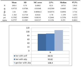
Mean SD MC error 2.5% Median 97.5%
N 108.4 9.74 0.6063 92.0 107.0 130.0
α
0.9735 0.9788 0.01048 0.02589 0.6685 3.681β
1.01 1.002 0.009612 0.02574 0.6994 3.716mu -1.363 0.1718 0.0161 -1.78 -1.359 -1.071 psi 0.3382 0.04004 0.00191 0.2646 0.3356 0.4252 sigma 0.2757 0.1283 0.01217 0.1156 0.251 0.6041
N
70 100 125 150
0
.
0
0
.
0
4
N
71 80 100 120 140
0
.
0
0
.
0
4
N
81 100 120 140
0
.
0
0
.
0
4
Fig 2a Model I Fig 2b Model II Fig 2c Model III
Fig 2 Comparisons of the size of the closed population estimate N between models I, II, and III
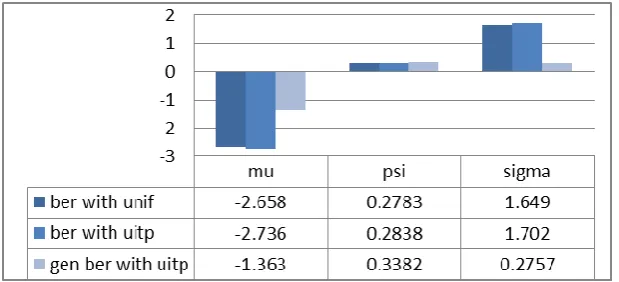
Fig 3 Comparisons of bird breeding data estimates between models I, II, and III
Examination of the above simulations (Tables 3.1–3.6 and Figures 1-3) yields the following observations:
1. The posterior mean of the estimate N of models I, II, and III are 88.92, 90.82, and 108.4, respectively. There is a clear and substantial shift of the posterior mean to the right. The posterior standard deviation (SD) is 10.57, 11.82 and 9.74, respectively, and hence a slight change in posterior SD. Comparison of the MC error for model I, II and III shows also a slight change in MC error.
2. The posterior mean of the estimate mu of models I, II, and III are -2.658, -2.736 and -1.363, respectively. There is a slight shift of the posterior mean to the right. The posterior standard deviation (SD) is 0.4078, 0.4404 and 0.1718, respectively, and hence a slight shift to the left in posterior SD. Comparison of the MC error for model I, II and III shows a slight change in MC error.
3. The posterior mean of the estimate psi of models I, II, and III are 0.2783, 0.2838 and 0.3382, respectively. There is a slight shift of the posterior mean to the right. The posterior standard deviation (SD) is 0.04101, 0.04488 and 0.04004, respectively, and hence it shows that they are about the same in posterior SD. Comparison of the MC error for model I, II and III shows a slight change in MC error.
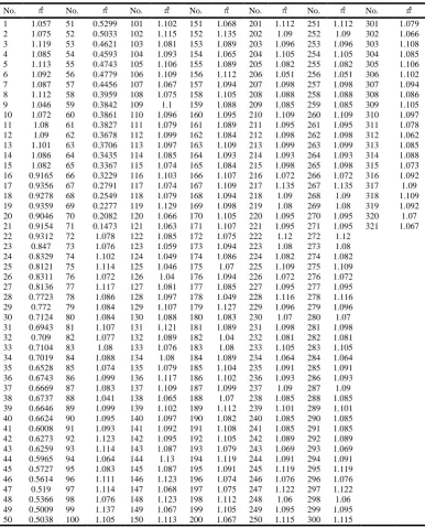
Table 3.4 Bayesian summary estimates for π, when π> 0, for model III
No. No. No. No. No. No. No.
1 1.057 51 0.5299 101 1.102 151 1.068 201 1.112 251 1.112 301 1.079 2 1.075 52 0.5033 102 1.115 152 1.135 202 1.09 252 1.09 302 1.066 3 1.119 53 0.4621 103 1.081 153 1.089 203 1.096 253 1.096 303 1.108 4 1.085 54 0.4593 104 1.093 154 1.065 204 1.105 254 1.105 304 1.085 5 1.113 55 0.4743 105 1.106 155 1.089 205 1.082 255 1.082 305 1.106 6 1.092 56 0.4779 106 1.109 156 1.112 206 1.051 256 1.051 306 1.102 7 1.087 57 0.4456 107 1.067 157 1.094 207 1.098 257 1.098 307 1.094 8 1.112 58 0.3959 108 1.075 158 1.105 208 1.088 258 1.088 308 1.086 9 1.046 59 0.3842 109 1.1 159 1.088 209 1.085 259 1.085 309 1.105 10 1.072 60 0.3861 110 1.096 160 1.095 210 1.109 260 1.109 310 1.097 11 1.08 61 0.3827 111 1.079 161 1.089 211 1.095 261 1.095 311 1.078 12 1.09 62 0.3678 112 1.099 162 1.084 212 1.098 262 1.098 312 1.062 13 1.101 63 0.3706 113 1.097 163 1.109 213 1.099 263 1.099 313 1.085 14 1.086 64 0.3435 114 1.085 164 1.093 214 1.093 264 1.093 314 1.088 15 1.082 65 0.3367 115 1.074 165 1.084 215 1.098 265 1.098 315 1.073 16 0.9165 66 0.3229 116 1.103 166 1.107 216 1.072 266 1.072 316 1.092 17 0.9356 67 0.2791 117 1.074 167 1.109 217 1.135 267 1.135 317 1.09 18 0.9278 68 0.2549 118 1.079 168 1.094 218 1.09 268 1.09 318 1.109 19 0.9359 69 0.2277 119 1.129 169 1.098 219 1.08 269 1.08 319 1.092 20 0.9046 70 0.2082 120 1.066 170 1.105 220 1.095 270 1.095 320 1.07 21 0.9154 71 0.1473 121 1.063 171 1.107 221 1.095 271 1.095 321 1.067 22 0.9312 72 1.078 122 1.085 172 1.075 222 1.12 272 1.12
23 0.847 73 1.076 123 1.059 173 1.094 223 1.08 273 1.08 24 0.8329 74 1.102 124 1.049 174 1.086 224 1.082 274 1.082 25 0.8121 75 1.114 125 1.046 175 1.07 225 1.109 275 1.109 26 0.8311 76 1.072 126 1.04 176 1.094 226 1.072 276 1.072 27 0.8136 77 1.117 127 1.081 177 1.085 227 1.095 277 1.095 28 0.7723 78 1.086 128 1.097 178 1.049 228 1.116 278 1.116 29 0.772 79 1.084 129 1.107 179 1.127 229 1.096 279 1.096 30 0.7124 80 1.084 130 1.088 180 1.083 230 1.07 280 1.07 31 0.6943 81 1.107 131 1.121 181 1.089 231 1.098 281 1.098 32 0.709 82 1.077 132 1.089 182 1.04 232 1.081 282 1.081 33 0.7104 83 1.08 133 1.076 183 1.08 233 1.105 283 1.105 34 0.7019 84 1.088 134 1.08 184 1.089 234 1.064 284 1.064 35 0.6528 85 1.074 135 1.079 185 1.104 235 1.091 285 1.091 36 0.6743 86 1.099 136 1.117 186 1.102 236 1.093 286 1.093 37 0.6669 87 1.083 137 1.109 187 1.099 237 1.09 287 1.09 38 0.6737 88 1.041 138 1.065 188 1.07 238 1.085 288 1.085 39 0.6646 89 1.099 139 1.102 189 1.112 239 1.101 289 1.101 40 0.6624 90 1.095 140 1.097 190 1.082 240 1.085 290 1.085 41 0.6008 91 1.093 141 1.092 191 1.108 241 1.085 291 1.085 42 0.6273 92 1.123 142 1.095 192 1.105 242 1.089 292 1.089 43 0.6259 93 1.114 143 1.087 193 1.079 243 1.069 293 1.069 44 0.5965 94 1.064 144 1.13 194 1.119 244 1.091 294 1.091 45 0.5727 95 1.083 145 1.087 195 1.091 245 1.119 295 1.119 46 0.5614 96 1.111 146 1.123 196 1.074 246 1.076 296 1.076 47 0.519 97 1.114 147 1.068 197 1.075 247 1.122 297 1.122 48 0.5366 98 1.076 148 1.123 198 1.112 248 1.06 298 1.06 49 0.5009 99 1.137 149 1.067 199 1.105 249 1.095 299 1.095 50 0.5038 100 1.105 150 1.113 200 1.067 250 1.115 300 1.115
5. The posterior mean of the estimate α of models II, and III are 1.069, and 0.9735, respectively. There is a clear shift of the posterior mean to the left. The posterior standard deviation (SD) is 1.112, and 0.9788, respectively, and hence a decrease in posterior SD. Comparison of the MC error for II, III shows that they are about the same.
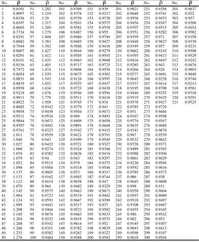
Table 3.5 Bayesian summary estimates for ρ, when ρ 0, for model III
No. No. No. No. No. No. No.
1 0.8161 51 1.282 101 0.9369 151 0.939 201 0.9821 251 0.9356 301 0.9637 2 0.8097 52 1.219 102 0.9376 152 0.9217 202 0.9648 252 0.9741 302 0.922 3 0.8336 53 1.29 103 0.9759 153 0.9738 203 0.9558 253 0.9453 303 0.957 4 0.8107 54 1.317 104 0.9541 154 0.9575 204 0.9456 254 0.9347 304 0.9306 5 0.8065 55 1.269 105 0.9581 155 0.9558 205 0.9707 255 0.9515 305 0.9454 6 0.7734 56 1.279 106 0.9487 156 0.955 206 0.9551 256 0.9282 306 0.9582 7 0.8291 57 1.404 107 0.9486 157 0.9704 207 0.9399 257 0.971 307 0.9358 8 0.8682 58 1.383 108 0.9485 158 0.9427 208 0.9448 258 0.9627 308 0.9339 9 0.7944 59 1.392 109 0.9506 159 0.9436 209 0.9349 259 0.957 309 0.9231 10 0.8007 60 1.427 110 0.9644 160 0.9279 210 0.9662 260 0.9245 310 0.9508 11 0.8201 61 1.412 111 0.9505 161 0.9545 211 0.9395 261 0.9413 311 0.9529 12 0.8101 62 1.425 112 0.9463 162 0.9668 212 0.9416 262 0.9447 312 0.9242 13 0.8156 63 1.401 113 0.9717 163 0.9725 213 0.9285 263 0.943 313 0.9476 14 0.7972 64 1.474 114 0.9606 164 0.9556 214 0.9266 264 0.926 314 0.9603 15 0.8054 65 1.529 115 0.9675 165 0.9302 215 0.9277 265 0.9681 315 0.9649 16 0.8831 66 1.545 116 0.9126 166 0.9597 216 0.9645 266 0.9238 316 0.9746 17 0.8839 67 1.652 117 0.9555 167 0.9457 217 0.9337 267 0.9414 317 0.9213 18 0.8958 68 1.634 118 0.9723 168 0.9438 218 0.9195 268 0.9708 318 0.9581 19 0.9218 69 1.676 119 0.9546 169 0.9594 219 0.9446 269 0.9252 319 0.9316 20 0.9011 70 1.779 120 0.9511 170 0.9418 220 0.9519 270 0.9425 320 0.9291 21 0.8822 71 1.958 121 0.9745 171 0.934 221 0.9578 271 0.9427 321 0.9525 22 0.8685 72 0.9342 122 0.9379 172 0.941 222 0.9785 272 0.9729
23 0.9858 73 0.9458 123 0.9564 173 0.9471 223 0.951 273 0.9464 24 0.9511 74 0.9534 124 0.969 174 0.9493 224 0.9167 274 0.9598 25 0.9844 75 0.9471 125 0.9409 175 0.9458 225 0.9774 275 0.9547 26 0.9707 76 0.9492 126 0.9891 176 0.9648 226 0.9635 276 0.9689 27 0.9761 77 0.9323 127 0.9342 177 0.9415 227 0.9341 277 0.9676 28 1.011 78 0.9559 128 0.9421 178 0.9791 228 0.967 278 0.9539 29 1.046 79 0.943 129 0.9399 179 0.9549 229 0.9532 279 0.9642 30 1.027 80 0.9423 130 0.9721 180 0.9327 230 0.9728 280 0.9371 31 1.068 81 0.9274 131 0.9324 181 0.9346 231 0.9489 281 0.9365 32 1.076 82 0.9382 132 0.9626 182 0.9434 232 0.9588 282 0.9306 33 1.079 83 0.94 133 0.943 183 0.9297 233 0.9661 283 0.9629 34 1.052 84 0.9515 134 0.979 184 0.9375 234 0.9226 284 0.9594 35 1.098 85 0.9584 135 0.9318 185 0.9546 235 0.9592 285 0.9616 36 1.137 86 0.9605 136 0.953 186 0.9317 236 0.9785 286 0.9375 37 1.133 87 0.9162 137 0.9403 187 0.9744 237 0.986 287 0.938 38 1.112 88 0.9414 138 0.9658 188 0.947 238 0.9645 288 0.9608 39 1.079 89 0.964 139 0.9482 189 0.9329 239 0.998 289 0.931 40 1.145 90 0.9575 140 0.9463 190 0.9671 240 0.9558 290 0.9604 41 1.094 91 0.9723 141 0.9519 191 0.9402 241 0.9597 291 0.9089 42 1.124 92 0.9593 142 0.9667 192 0.9399 242 0.9518 292 0.9497 43 1.099 93 0.9443 143 0.9317 193 0.937 243 0.9708 293 0.9467 44 1.208 94 0.9464 144 0.9522 194 0.9502 244 0.9455 294 0.9165 45 1.165 95 0.9676 145 0.9463 195 0.9433 245 0.986 295 0.9542 46 1.204 96 0.9232 146 0.9419 196 0.9575 246 0.962 296 0.953 47 1.268 97 0.9342 147 0.9614 197 0.952 247 0.9145 297 0.9307 48 1.266 98 0.9351 148 0.9782 198 0.9829 248 0.9043 298 0.9413 49 1.233 99 0.9382 149 0.9262 199 0.9322 249 0.9598 299 0.9347 50 1.276 100 0.9464 150 0.9588 200 0.9582 250 0.9618 300 0.9504
7. The posterior mean of the estimate π of models III (table 3.4) vary between (0.1473, 1.37). This indicate that the data are effected by the generalized model III. These findings do not sport the work done by [[2] Royle and Dorazio (2008), Chapter 6]. Who use SBM(n,p). We also note the following interesting readings that bird (No. 71) has the lowest estimated value α at 0.1473, with highest number of observed detection at 36 readings. This maybe, related to the factor effect of behavior and/or biology of the bird.
Table 3.6 Bayesian summary estimates for τ, when τ 0, for model III
No. No. No. No. No. No. No.
1 1.094 51 0.4792 101 1.058 151 1.12 201 1.082 251 1.092 301 1.073 2 1.107 52 0.4712 102 1.089 152 1.081 202 1.089 252 1.095 302 1.12 3 1.049 53 0.469 103 1.089 153 1.064 203 1.067 253 1.1 303 1.07 4 1.062 54 0.4974 104 1.073 154 1.058 204 1.111 254 1.09 304 1.08 5 1.056 55 0.473 105 1.057 155 1.113 205 1.086 255 1.102 305 1.104 6 1.032 56 0.4776 106 1.103 156 1.094 206 1.068 256 1.117 306 1.111 7 1.071 57 0.4419 107 1.103 157 1.105 207 1.071 257 1.099 307 1.09 8 1.094 58 0.3994 108 1.083 158 1.104 208 1.078 258 1.113 308 1.089 9 1.09 59 0.4168 109 1.131 159 1.129 209 1.085 259 1.151 309 1.112 10 1.073 60 0.3754 110 1.113 160 1.094 210 1.069 260 1.094 310 1.075 11 1.092 61 0.3774 111 1.081 161 1.069 211 1.081 261 1.082 311 1.073 12 1.061 62 0.4018 112 1.084 162 1.104 212 1.089 262 1.093 312 1.106 13 1.071 63 0.3707 113 1.069 163 1.094 213 1.097 263 1.108 313 1.09 14 1.059 64 0.3635 114 1.101 164 1.098 214 1.099 264 1.085 314 1.096 15 1.079 65 0.3677 115 1.083 165 1.084 215 1.094 265 1.079 315 1.105 16 0.878 66 0.3459 116 1.097 166 1.093 216 1.093 266 1.074 316 1.074 17 0.8868 67 0.3 117 1.068 167 1.103 217 1.109 267 1.079 317 1.103 18 0.9047 68 0.2873 118 1.085 168 1.089 218 1.089 268 1.102 318 1.135 19 0.9043 69 0.2746 119 1.068 169 1.083 219 1.082 269 1.102 319 1.111 20 0.9167 70 0.2686 120 1.077 170 1.107 220 1.084 270 1.115 320 1.109 21 0.9005 71 0.2235 121 1.107 171 1.109 221 1.058 271 1.116 321 1.081 22 0.8803 72 1.086 122 1.11 172 1.08 222 1.114 272 1.076
23 0.7933 73 1.134 123 1.107 173 1.081 223 1.118 273 1.115 24 0.8018 74 1.096 124 1.088 174 1.101 224 1.071 274 1.094 25 0.8243 75 1.092 125 1.096 175 1.08 225 1.092 275 1.125 26 0.7889 76 1.105 126 1.077 176 1.074 226 1.088 276 1.024 27 0.806 77 1.108 127 1.111 177 1.115 227 1.087 277 1.098 28 0.7128 78 1.102 128 1.098 178 1.099 228 1.106 278 1.09 29 0.7147 79 1.081 129 1.093 179 1.078 229 1.075 279 1.071 30 0.6464 80 1.096 130 1.122 180 1.108 230 1.109 280 1.106 31 0.6815 81 1.094 131 1.09 181 1.088 231 1.133 281 1.065 32 0.6848 82 1.112 132 1.086 182 1.125 232 1.152 282 1.108 33 0.6795 83 1.132 133 1.071 183 1.093 233 1.097 283 1.085 34 0.6768 84 1.104 134 1.129 184 1.141 234 1.084 284 1.083 35 0.6416 85 1.101 135 1.109 185 1.107 235 1.071 285 1.121 36 0.6329 86 1.058 136 1.108 186 1.089 236 1.109 286 1.131 37 0.6412 87 1.1 137 1.127 187 1.117 237 1.11 287 1.08 38 0.6259 88 1.111 138 1.083 188 1.117 238 1.114 288 1.111 39 0.6234 89 1.142 139 1.096 189 1.061 239 1.086 289 1.124 40 0.6357 90 1.081 140 1.073 190 1.118 240 1.091 290 1.089 41 0.5896 91 1.092 141 1.102 191 1.06 241 1.101 291 1.13 42 0.5828 92 1.082 142 1.086 192 1.072 242 1.06 292 1.135 43 0.5716 93 1.104 143 1.082 193 1.092 243 1.114 293 1.052 44 0.5832 94 1.129 144 1.141 194 1.098 244 1.1 294 1.101 45 0.5836 95 1.094 145 1.109 195 1.093 245 1.081 295 1.071 46 0.5348 96 1.1 146 1.129 196 1.072 246 1.071 296 1.108 47 0.5363 97 1.092 147 1.073 197 1.083 247 1.108 297 1.089 48 0.5127 98 1.103 148 1.091 198 1.101 248 1.096 298 1.052 49 0.4916 99 1.121 149 1.118 199 1.079 249 1.092 299 1.073 50 0.4987 100 1.107 150 1.103 200 1.094 250 1.069 300 1.085
9. The posterior mean of the estimate τ of models III (table 3.6) vary between (0.2235, 1.152). This indicate that the data are effected by the generalized model III. These findings do not sport the work done by [[2] Royle and Dorazio (2008), Chapter 6]. Who use SBM(n,p). We also note the following interesting reading that bird (No. 71) has the lowest estimated value α at 0.2235, with highest number of observed detection at 36 readings.
Royle and Dorazio (2008), Chapter 6]. The proposed class of generalized models thrust and interject more flexibility, litheness, and resilience, for Bayesian methods to choose among the existing classes of models.
IV. CONCLUSION
In this paper we examined the influence of having generalized models as an alternative model to the standard models. We have shown the importance and usefulness of the new models through the bird breeding survey (BBS) data set. Another feature of proposed generalized models is that under Bayesian perspective, it generalize the posterior of the parameters to predict the behavior and biology effect of the birds which make the generalized models more intrinsic and litheness. Unlike the work of [[2] Royle and Dorazio (2008), Chapter 6] who confined and limited there work only on standard models to analyse the bird breeding data. The present study will aid in identifying some problems involving uncertain events in ecology, and gives an efficient computational Bayesian approach with new ways of predicting and measuring behavior factors.
ACKNOWLEDGMENTS
The support by the Research Administration, Kuwait University, Kuwait, is acknowledged by the first author.
APPENDIX
The data set bellow (Table A) follows that of [[2] Royle and Dorazio (2008), Chapter 6]. It consists of observed detections for 71 birds in a Breeding Bird Survey (BBS) study in Maryland.
Table A
1 1 1 1 1 1 1 1 1 1 1 1 1 1 1 2 2 2
2 2 2 2 3 3 3 3 3 4 4 5 5 5 5 5 6 6
6 6 6 6 7 7 7 8 8 9 10 10 11 11 11 11 12 12
12 12 14 16 16 17 17 17 18 19 20 21 25 26 28 30 36 0
0 0 0 0 0 0 0 0 0 0 0 0 0 0 0 0 0 0
0 0 0 0 0 0 0 0 0 0 0 0 0 0 0 0 0 0
0 0 0 0 0 0 0 0 0 0 0 0 0 0 0 0 0 0
0 0 0 0 0 0 0 0 0 0 0 0 0 0 0 0 0 0
0 0 0 0 0 0 0 0 0 0 0 0 0 0 0 0 0 0
0 0 0 0 0 0 0 0 0 0 0 0 0 0 0 0 0 0
0 0 0 0 0 0 0 0 0 0 0 0 0 0 0 0 0 0
0 0 0 0 0 0 0 0 0 0 0 0 0 0 0 0 0 0
0 0 0 0 0 0 0 0 0 0 0 0 0 0 0 0 0 0
0 0 0 0 0 0 0 0 0 0 0 0 0 0 0 0 0 0
0 0 0 0 0 0 0 0 0 0 0 0 0 0 0 0 0 0
0 0 0 0 0 0 0 0 0 0 0 0 0 0 0 0 0 0
0 0 0 0 0 0 0 0 0 0 0 0 0 0 0 0 0 0
0 0 0 0 0 0 0 0 0 0 0 0 0 0 0
REFERENCES
[1] J. A. Al-Saleh, S. K. Agarwal, and R. Al-Bannay “EuroSCORE overestimated cardiac surgery related mortality: Comparing EuroSCORE model and Bayesian approach using new generalized probabilistic model with new form of prior information,”
International Journal of Medical Science, 3(12), 1-12. 2016.
[2] J. Royle, and R. Dorazio, “Hierarchical Modeling and Inference in Ecology: The Analysis of Data from Populations, Metapopulations and Communities.” First edition. Academic Press. 2008.
[3] J. A. Al-Saleh, S. K. Agarwal “Extended Weibull type distribution and finite mixture of distributions,” Statistical Methodology, 3, 224-233. 2006.
[4] J. A. Al-Saleh, and S. K. Agarwal “Reliability Prediction Updating Through Computational Bayesian for Mixed and Non-mixed Lifetime Data Using More Flexible New Extra Modified Weibull Model,” American Scientific Research Journal for Engineering, Technology, and Sciences, 38(1), 283-292. 2017.
[5] R. King, and S. P. Brooks “On the Bayesian analysis of population size” Biometrika, vol. 88(2), pp. 317-336. 2001.
[6] J. A. Royle, R. M. Dorazio, and W. N. Link “Analysis of Multinomial Models with Unknown Index Using Data Augmentation.”
Journal of Computational and Graphical Statistics. vol. 16(1), pp. 67-85. 2007.
[7] M. S. C. S. Limaa, J. Pederassib, and C. A. S. Souzac “Estimation of a closed population size of tadpoles in temporary pond.”
Brazelian Journal Biology, vol. 78(2), pp. 328-336. 2018.