On Generalized Bellman Equations and
Temporal-Difference Learning
Huizhen Yu [email protected]
Reinforcement Learning and Artificial Intelligence Group Department of Computing Science, University of Alberta Edmonton, AB, T6G 2E8, Canada
A. Rupam Mahmood [email protected]
Kindred Inc. 243 College St
Toronto, ON M5T 1R5, Canada
Richard S. Sutton [email protected]
Reinforcement Learning and Artificial Intelligence Group Department of Computing Science, University of Alberta Edmonton, AB, T6G 2E8, Canada
Editor:Csaba Szepesv´ari
Abstract
We consider off-policy temporal-difference (TD) learning in discounted Markov decision processes, where the goal is to evaluate a policy in a model-free way by using observations of a state process generated without executing the policy. To curb the high variance issue in off-policy TD learning, we propose a new scheme of setting the λ-parameters of TD, based on generalized Bellman equations. Our scheme is to setλaccording to the eligibility trace iterates calculated in TD, thereby easily keeping these traces in a desired bounded range. Compared with prior work, this scheme is more direct and flexible, and allows much largerλvalues for off-policy TD learning with bounded traces. As to its soundness, using Markov chain theory, we prove the ergodicity of the joint state-trace process under nonrestrictive conditions, and we show that associated with our scheme is a generalized Bellman equation (for the policy to be evaluated) that depends on both the evolution ofλ
and the unique invariant probability measure of the state-trace process. These results not only lead immediately to a characterization of the convergence behavior of least-squares based implementation of our scheme, but also prepare the ground for further analysis of gradient-based implementations.
Keywords: Markov decision process, approximate policy evaluation, generalized Bellman equation, reinforcement learning, temporal-difference method, Markov chain, randomized stopping time
1. Introduction
We consider discounted Markov decision processes (MDPs) and off-policy temporal-difference (TD) learning methods for approximate policy evaluation with linear function
approxima-c
tion. The goal is to evaluate a policy in a model-free way by using observations of a state process generated without executing the policy. Off-policy learning is an important part of the reinforcement learning methodology (Sutton and Barto, 1998) and has been studied in the areas of operations research and machine learning. (For an incomplete list of references, see e.g., Glynn and Iglehart, 1989; Precup et al., 2000, 2001; Randhawa and Juneja, 2004; Sutton et al., 2008, 2009; Maei, 2011; Yu, 2012; Dann et al., 2014; Geist and Scherrer, 2014; Mahadevan et al., 2014; Mahmood et al., 2014; Liu et al., 2015; Sutton et al., 2016; Dai et al., 2018.) Available TD algorithms, however, tend to have very high variances due to the use of importance sampling, an issue that limits their applicability in practice. The purpose of this paper is to introduce a new TD learning scheme that can help address this problem.
Our work is motivated by the recently proposed Retrace algorithm (Munos et al., 2016) and ABQ algorithm (Mahmood et al., 2017), and by the Tree-Backup algorithm (Precup et al., 2000) that existed earlier. These algorithms, as explained by Mahmood et al. (2017), all try to use theλ-parameters of TD to curb the high variance issue in off-policy learning. In particular, they all choose the values of λaccording to the current state or state-action pair in such a way that guarantees the boundedness of the eligibility traces in TD learning, which can help reduce significantly the variance of the TD iterates. A limitation of these algorithms, however, is that they tend to be over-conservative and restrictλto small values, whereas small λcan result in large approximation bias in TD solutions.
In this paper, we propose a new scheme of setting the λ-parameters of TD, based on generalized Bellman equations. Our scheme is to set λ according to the eligibility trace iterates calculated in TD, thereby easily keeping those traces in a desired bounded range. Compared with the schemes used in the previous work just mentioned, this is a direct way to bound the traces in TD, and it is also more flexible and allows much larger λvalues for off-policy learning.
Regarding generalized Bellman equations, in our context, they will correspond to a fam-ily of dynamic programming equations for the policy to be evaluated. These equations all have the true value function as their unique solution, and their associated operators have contraction properties, like the standard Bellman operator. We will refer to the associated operators as generalized Bellman operators or Bellman operators for short. Some authors have considered, at least conceptually, the use of an even broader class of equations for policy evaluation. For example, Ueno et al. (2011) have considered treating the policy evaluation problem as a parameter estimation problem in the statistical framework of esti-mating equations, and in their framework, any equation that has the true value function as the unique solution can be used to estimate the value function. The family of generalized Bellman equations we consider has a more specific structure. They generalize multistep Bellman equations, and they are associated with randomized stopping times and arise from the strong Markov property (see Section 3.1 for details).
to different Bellman operators. Early efforts that use this aspect to broaden the scope of TD algorithms and to analyze such algorithms include Sutton’s work (1995) on learning at multiple timescales and Tsitsiklis’ work on generalized TD algorithms in the tabular case (see the book by Bertsekas and Tsitsiklis, 1996, Chap. 5.3). In the context of off-policy learning, there are more recent approaches that try to utilize this connection of TD with generalized Bellman operators to make TD learning more efficient (Precup et al., 2000; Yu and Bertsekas, 2012; Munos et al., 2016; Mahmood et al., 2017). This is also our aim, in proposing the new scheme of setting the λ-parameters.
Our analyses of the new TD learning scheme will focus on its theoretical side. Using Markov chain theory, we prove the ergodicity of the joint state and trace process under nonrestrictive conditions (see Theorem 2.1), and we show that associated with our scheme is a generalized Bellman equation (for the policy to be evaluated) that depends on both the evolution of λ and the unique invariant probability measure of the state-trace process (see Theorem 3.2 and Corollary 3.1). These results not only lead immediately to a charac-terization of the convergence behavior of least-squares based implementation of our scheme (see Corollary 2.1 and Remark 3.2), but also prepare the ground for further analysis of gradient-based implementations. (The latter analysis has been carried out recently by Yu (2017); see Remark 3.3.)
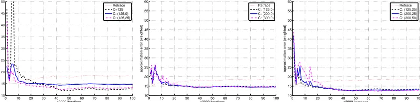
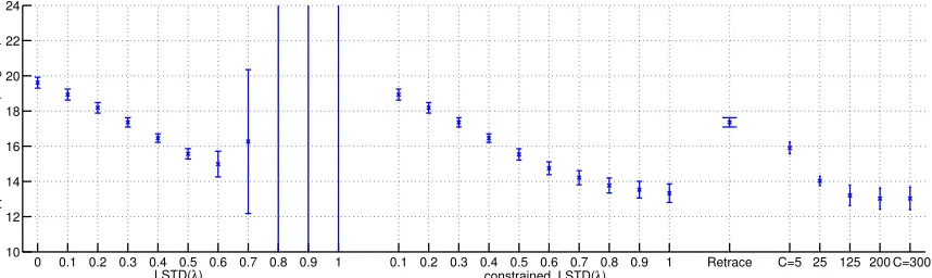
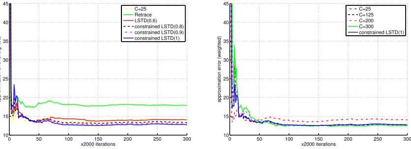
In addition to the theoretical study, we also present the results from a preliminary numerical study that compares several ways of setting λ for the least-squares based off-policy algorithm. The results demonstrate the advantages of the proposed new scheme with its greater flexibility.
We remark that although we shall focus exclusively on policy evaluation in this paper, approximate policy evaluation methods are highly pertinent to finding near-optimal policies in MDPs. They can be applied in approximate policy iteration, in policy-gradient algorithms for gradient estimation or in direct policy search (see e.g., Konda, 2002; Mannor et al., 2003). In addition to solving MDPs, they can also be used in artificial intelligence and robotics applications as a means to generate experience-based world models (see e.g., Sutton, 2009). It is, however, beyond the scope of this paper to discuss these applications of our results.
The rest of the paper is organized as follows. In Section 2, after a brief background in-troduction, we present our scheme of TD learning with bounded traces, and we establish the ergodicity of the joint state-trace process. In Section 3, we first discuss generalized Bellman operators associated with randomized stopping times, and we then derive the generalized Bellman equation associated with our scheme. In Section 4, we present the experimental results on the least-squares based implementation of our scheme. Appendices A-B include a proof for generalized Bellman operators and materials about approximation properties of TD solutions that are too long to include in the main text.
2. Off-Policy TD Learning with Bounded Traces
2.1 Preliminaries
The off-policy learning problem we consider in this paper concerns two Markov chains on a finite state spaceS ={1, . . . , N}. The first chain has transition matrixP, and the second
Po. Whatever physical mechanisms that induce the two chains shall be denoted byπandπo, and referred to as the target policy and behavior policy, respectively. The second Markov chain we can observe; however, it is the system performance of the first Markov chain that we want to evaluate.
Specifically, we consider a one-stage reward function rπ : S → < and an associated discounted total reward criterion with state-dependent discount factors γ(s)∈[0,1], s∈ S. Let Γ denote theN×N diagonal matrix with diagonal entriesγ(s). We assume thatP and
Po satisfy the following conditions:
Condition 2.1 (Conditions on the target and behavior policies)
(i) P is such that the inverse(I−PΓ)−1 exists, and
(ii) Po is such that for all s, s0 ∈ S,Psso0 = 0⇒Pss0 = 0, and moreover,Po is irreducible.
The performance ofπis defined as the expected discounted total rewards for each initial states∈ S:
vπ(s) :=Eπs[rπ(S0) +P∞t=1γ(S1)γ(S2) · · · γ(St)·rπ(St)], (2.1) where the notation Eπ
s means that the expectation is taken with respect to (w.r.t.) the Markov chain {St} starting fromS0 =sand induced by π (i.e., with transition matrixP). The function vπ is well-defined under Condition 2.1(i). It is called thevalue function of π, and by standard MDP theory (see e.g., Puterman, 1994), we can write it in matrix/vector notation as
vπ =rπ+PΓvπ, i.e., vπ = (I−PΓ)−1rπ.
The first equation above is known as the Bellman equation (or dynamic programming equation) for a stationary policy (cf. Footnote 2).
We compute an approximation of vπ of the form v(s) =φ(s)>θ, s ∈ S, where θ ∈ <n is a parameter vector and φ(s) is ann-dimensional feature representation for each states
(hereφ(s), θ are column vectors and the symbol>stands for transpose). Data available for this computation are:
(i) a realization of the Markov chain {St} with transition matrix Po generated by πo, and
(ii) rewardsRt=r(St, St+1) associated with state transitions, where the functionrrelates torπ(s) as rπ(s) =Eπs[r(s, S1)] for alls∈ S.1
To find a suitable parameter θ for the approximation φ(s)>θ, we use the off-policy TD learning scheme. Define ρ(s, s0) =Pss0/Po
ss0 (the importance sampling ratio),2 and write ρt=ρ(St, St+1), γt=γ(St).
1. One can add toRt a zero-mean finite-variance noise term. This makes little difference to our analyses,
so we have left it out for notational simplicity.
2. Our problem formulation entails both value function and state-action value function estimation for a stationary policy in the standard MDP context. In these applications, it is the state-action space of the
Given an initiale0 ∈ <n, for each t≥1, the eligibility trace vector et∈ <n and the scalar temporal-difference termδt(v) for any approximate value functionv:S → <are calculated according to
et=λtγtρt−1et−1+φ(St), (2.2)
δt(v) =ρt Rt+γt+1v(St+1)−v(St)
. (2.3)
Here λt ∈ [0,1], t ≥ 1, are important parameters in TD learning, the choice of which we shall elaborate on shortly.
There exist a number of TD algorithms that use et and δt to generate a sequence of parametersθtfor approximate value functions. One such algorithm is LSTD (Boyan, 1999; Yu, 2012), which obtainsθt by solving the linear equation forθ∈ <n,
1 t
Pt−1
k=0 ekδk(v) = 0, v = Φθ (2.4) (if it admits a solution), where Φ is a matrix with row vectorsφ(s)>, s∈ S. LSTD updates the equation (2.4) iteratively by incorporating one by one the observation of (St, St+1, Rt) at each state transition. We will discuss primarily this algorithm in the paper, as its behavior can be characterized directly using our subsequent analyses of the joint state-trace process. As mentioned earlier, our analyses will also provide bases for analyzing other gradient-based TD algorithms (e.g., Sutton et al., 2008, 2009; Maei, 2011; Mahadevan et al., 2014) by using stochastic approximation theory (Kushner and Yin, 2003; Borkar, 2008; Karmakar and Bhatnagar, 2018). Because of the complexity of this subject, however, we will not delve into it in the present paper, and we refer the reader to the recent work (Yu, 2017) for details.
2.2 Our Scheme of History-dependent λ
We now come to the choices ofλtin the trace iterates (2.2). For TD with function approxi-mation, one often letsλtbe a constant or a function ofSt(Sutton, 1988; Tsitsiklis and Van Roy, 1997; Sutton and Barto, 1998). If neither the behavior policy nor the λt’s are further constrained, {et} can have unbounded variances and is also unbounded in many natural situations (see e.g., Yu, 2012, Section 3.1), and this makes off-policy TD learning challeng-ing.3 If we let the behavior policy to be close enough to the target policy so that Po ≈P, then variance can be reduced, but it is not a satisfactory solution, for the applicability of off-policy learning would be seriously limited.
Without restricting the behavior policy, as mentioned earlier, the two recent papers (Munos et al., 2016; Mahmood et al., 2017), as well as the closely related early work by
corresponds to the pair of previous action and current state in the MDP, whereas for state-value function
estimation,Sthere corresponds to the current state-action pair in the MDP. The ratioρ(s, s0) =Pss0/Psso0
then comes out as the ratio of action probabilities underπandπo, the same as what appears in most of
the off-policy learning literature. For the details of these correspondences, see (Yu, 2012, Examples 2.1,
2.2). The third application is in a simulation context wherePo corresponds to a simulated system and
bothPo, P are known so that the ratioρ(s, s0
) is available. Such simulations are useful, for example, in studying system performance under perturbations, and in speeding up the computation when assessing
the impacts of events that are rare under the dynamicsP.
Precup et al. (2000), exploit state-dependent λ’s to control variance. Their choices of λt are such thatλtγtρt−1 <1 for allt, so that the trace iterates et are made bounded, which can help reduce the variance of the iterates.
Motivated by this prior work, our proposal is to setλtaccording toet−1 directly, so that we can keep et in a desired range straightforwardly and at the same time, allow a much larger range of values for the λ-parameters. As a simple example, if we use λt to scale the vector γtρt−1et−1 to be within a ball with some given radius, then we keep et always bounded.
In the rest of this paper, we shall focus on analyzing the iteration (2.2) with a particular choice of λt of the kind just mentioned. We want to be more general than the preceding simple example. However, since the dependence on the traceet−1would makeλtdependent on the entire past history (S0, . . . , St−1), we also want to retain certain Markovian properties that are very useful for convergence analysis. This leads us to consider λt being a certain
function of the previous trace and past states. More specifically, we will letλtbe a function of the previous trace et−1 and a certain memory state that is a summary of the states observed so far. The formulation is as follows.
2.2.1 Formulation and Examples
We denote the memory state at time t by yt. For simplicity, we assume that yt can only take values from a finite set M, and its evolution is Markovian: yt= g(yt−1, St) for some given function g. The joint process {(St, yt)} is then a simple finite-state Markov chain. Each yt is a function of the history (S0, . . . , St) and y0. We further require, besides the irreducibility of{St}(cf. Condition 2.1(ii)), that
Condition 2.2 (Evolution of memory states) Under the behavior policyπo, the Markov chain {(St, yt)} on S × Mhas a single recurrent class.
This recurrence condition is nonrestrictive: If the Markov chain has multiple recurrent classes, each recurrent class can be treated separately by using the same arguments we present in this paper. However, we remark that the finiteness assumption on M is a simplification. We choose to work with finiteMmainly for the reason that with the traces lying in a continuous space, to study the joint state and trace process, we need to resort to properties of Markov chains on infinite spaces. With an infinite M, we would need to introduce more technical conditions that are not essential to our analysis and can obscure our main arguments.
We thus let yt and λt evolve as
yt=g(yt−1, St), λt=λ(yt, et−1) (2.5)
whereλ:M × <n→[0,1]. We require the functionλto satisfy two conditions.
Condition 2.3 (Conditions for λ(·)) For some norm k · k on<n, the following hold for
each memory statey ∈ M:
(i) For any e, e0 ∈ <n, kλ(y, e)e−λ(y, e0)e0k ≤ ke−e0k.
(ii) For some constant Cy, kγ(s0)ρ(s, s0)·λ(y, e)ek ≤ Cy for all e∈ <n and all possible
In the above, the second condition is to restrict{et}in a desired range (as it makesketk ≤ maxy∈MCy+ maxs∈Skφ(s)k). The first condition is about the continuity of the function
λ(y, e)e in the trace variable e for each memory state y, and it plays a key role in the subsequent analysis, where we will use this condition to ensure that the traces et and the states (St, yt) jointly form a Markov chain with appealing properties. We shall defer a further discussion on the technical roles of these conditions to the end of Section 2.3 (cf. Remark 2.2).
Let us give a few simple examples of choosingλthat satisfy Condition 2.3. We will later use these examples in our experimental study (Section 4).
Example 2.1 We consider again the simple scaling example mentioned earlier and describe it using the terminologies just introduced. In this example, we letyt= (St−1, St). For each
y = (s, s0), we define the function λ(y,·) so that when multiplied with λ(y, e), the vector
γ(s0)ρ(s, s0)eis scaled down whenever its length exceeds a given thresholdCss0:
λ y, e= (
1 if γ(s0)ρ(s, s0)kek2≤Css0;
Css0
γ(s0)ρ(s,s0)kek
2 otherwise.
(2.6)
Condition 2.3(i) is satisfied because for y = (s, s0) with γ(s0)ρ(s, s0) = 0, λ y, e
e = e, whereas for y = (s, s0) with γ(s0)ρ(s, s0) 6= 0, λ y, e
e is simply the Euclidean projection of eonto the ball (centered at the origin) with radius Css0/(γ(s0)ρ(s, s0)) and is therefore
Lipschitz continuous in ewith modulus 1 w.r.t. k · k2. Corresponding to (2.6), the update rule (2.2) ofet becomes
et= (
γtρt−1et−1+φ(St) if γtρt−1ket−1k2 ≤CSt−1St; CSt−1St·
et−1
ket−1k2 +φ(St) otherwise.
(2.7)
Note that this scheme of setting λencourages the use of large λt: λt= 1 will be chosen whenever possible. A variation of the scheme is to multiply the right-hand side (r.h.s.) of (2.6) by another factor βss0 ∈ [0,1], so that λt can be at most βS
t−1St. In particular,
one such variation is to simply multiply the r.h.s. of (2.6) by a constant β ∈(0,1) so that
λt≤β <1 for allt.
Example 2.2 The Retrace algorithm (Munos et al., 2016) modifies the trace updates in off-policy TD learning by truncating the importance sampling ratios by 1. In particular, for the off-policy TD(λ) algorithm with a constant λ= β ∈ (0,1], Retrace modifies the trace updates to be
et=β γt·min{1, ρt−1} ·et−1+φ(St). (2.8) As pointed out by Mahmood et al. (2017), to retain the original interpretation of λ as a bootstrapping parameter in TD learning, we can rewrite the above update rule of Retrace equivalently as
et=λtγtρt−1et−1+φ(St) for λt=β·min{ρ1t−,ρ1t−1} (with 0/0 = 0). (2.9) Each λt here is a function of (St−1, St) only and does not depend on et−1, so this choice
(St−1, St). When the discount factors γ(s) are all strictly less than 1, ketk for all t are bounded by a deterministic constant that depends on the initial e0. Then for each initial
e0, Retrace’s choice of λcoincides with a choice in our framework, since theC-parameters in Condition 2.3(ii) can be made vacuously large so that the condition is satisfied by all the traces et that could be encountered by Retrace. Thus in this case our framework for choosingλeffectively encompasses the particular choice used by Retrace.
One can make variations on Retrace’s trace update rule. For example, instead of trun-cating each importance sampling ratio ρ(s, s0) by 1, one can truncate it by a constant
Kss0 ≥1, and then use a scaling scheme similar to Example 2.1 to bound the traces. The
simplest such variation is to choose two memory-independent positive constantsK and C, and replace the definition of λt in (2.9) by the following: with ˜λt= min{ρK,ρt−1t−1} (where we treat 0/0 = 0),
λt= (
βλ˜t if ˜λtγtρt−1ket−1k2≤C;
βλ˜t·λ˜tγtρt−C1ket−1k2 otherwise.
(2.10)
Correspondingly, instead of (2.8), the update rule ofet becomes
et= (
β γt·min{K, ρt−1} ·et−1+φ(St) if γt·min{K, ρt−1} · ket−1k2 ≤C;
β C· et−1
ket−1k2 +φ(St) otherwise.
(2.11)
These variations of Retrace are similar to Example 2.1 and satisfy Condition 2.3.4
2.2.2 Comparison with Previous Work
For policy evaluation, the Retrace algorithm (Munos et al., 2016) and the ABQ algorithm (Mahmood et al., 2017) are very similar (ABQ was actually developed independently of Retrace before the Munos et al. (2016) paper was published, although the ABQ paper itself was released much later). Both Retrace and ABQ include the Tree-Backup algorithm (Precup et al., 2000) as a special case. They can use additional parameters to selectλfrom a range of values, whereas Tree-Backup specifies λ, implicitly, in a particular way (which has the advantage of requiring no knowledge of the behavior policy) and does not have the freedom in choosingλ. Because of the relations between these algorithms, when comparing our method to them, we will compare it with Retrace only. In the experimental study given later in Section 4 on the performance of LSTD for various ways of settingλ, we will compare our scheme of choosingλwith that of Retrace forβ= 1, which lets Retrace use the largest
λthat it can take.
We see in Example 2.2 that the eligibility trace update rule of Retrace can be written in two equivalent forms, (2.8) and (2.9). The second form (2.9) has the advantage that theλ-parameters involved are shown explicitly. In TD learning, the λ-parameters directly affect the associated Bellman operators and can be meaningfully interpreted as stopping probabilities (see Section 3), whereas the importance sampling ratio terms in the eligibility
4. To see this, let the memory states beyt= (St−1, St). For eachy= (s, s0), letλ(y, e) be defined according
to (2.10), and let Cy in Condition 2.3(ii) be Css0 = ρ(s,s
0)
min{K, ρ(s,s0)}·C (treat 0/0 = 0). Then note that kλ(y, e)e−λ(y, e0)e0k2≤βmin
K
ρ(s,s0),1 · ke−e 0k
trace iterates are essentially unchanged, for they have to be there in order to correct for the discrepancy between the behavior and target policies. For this reason, we prefer (2.9) to (2.8) and prefer thinking in terms of the selection of λ-parameters to that of what occurs
apparently to those importance sampling ratio terms in the trace updates.
As mentioned in Example 2.2, the Munos et al. (2016) paper does not make the connec-tion between (2.8) and (2.9). Mahmood et al. (2017) recognized the role of theλ-parameters and made explicit use of it to derive the ABQ algorithm. However, in the ABQ paper, the discussion and the presentation of the algorithm still emphasize the apparent changes in those importance sampling ratio terms in the trace iterates. This is an unsatisfactory point in that paper that we hope we have clarified with our present work.
We mentioned in the introduction that Retrace, ABQ and Tree-Backup are too conser-vative and tend to use too small λ values. Let us now make this statement more precise and also explain the reason behind.
These algorithms tend to behave effectively like TD(λ) with small constant λ, despite that they can have λt = 1 at some time steps t. This is due to the nature of TD learning with time-varying λ, which is very different from that of TD with constant λ. For time-varying λ, a large λt at one time step need not mean that we are using the information of the cumulative rewards over a long time horizon to estimate the value at the state St encountered at time t. Because the next λt+1 could be very small or even zero, forcing a TD algorithm to “bootstrap” immediately. When largeλt’s are interleaved with small ones, we are effectively in the situation of TD with small λ. This could occur to our proposed scheme as well if, for example, in Example 2.1 the thresholdsCss0 are set too small. When we
use larger thresholds, we allow larger λ. By comparison, Retrace, ABQ, and Tree-Backup constrain the state-dependent λ-parameters to be small enough so that all the products
λtγtρt−1 < 1, and this makes them prone to the small-λ issue just mentioned. (See the experiments in Section 4.2 for demonstrations.)
While we consider Retrace for approximate policy evaluation, the Munos et al. (2016) paper actually focuses primarily on finding an optimal policy for an MDP, in the tabular case, and it has demonstrated good empirical performance of Retrace and Tree-Backup for that purpose. Despite this, its results are not adequate yet to establish asymptotic optimality of these algorithms in the online optimistic policy iteration setting (personal communication with Munos), and it is still an open theoretical question whether online TD algorithms can solve an MDP like the Q-learning algorithm (Watkins, 1989; Tsitsiklis, 1994), when positiveλ(small or not) and rapidly changing target policies are involved.
We also mention that for policy evaluation, Munos et al. (2016, Section 3.1) have also conceived the use of generalized Bellman operators, although they did not relate these operators explicitly to history-dependent λ’s and did not study corresponding algorithms in this general case.
2.3 Ergodicity Result
2017), although in this paper we discuss only the LSTD algorithm. In the next section we will also use the ergodicity result when we relate the LSTD equation (2.4) to a generalized Bellman equation for the target policy in order to interpret the LSTD solutions.
We note that to obtain the results in this subsection, we will follow similar lines of argument used in (Yu, 2012) for analyzing off-policy LSTD with constant λ. However, because λ is now history-dependent, some proof steps in (Yu, 2012) no longer apply. We shall explain this in more detail after we prove the main result of this subsection.
As another side note, one can introduce nonnegative coefficientsi(y) for memory states
y to weight the state features (similarly to the use of “interest” weights in the ETD algo-rithm (Sutton et al., 2016)) and update et according to
et=λtγtρt−1et−1+i(yt)φ(St). (2.12) The results given below apply to this update rule as well.
Let us start with two basic properties of{(St, yt, et)}that follow directly from our choice of the λfunction:
(i) By Condition 2.3(i), for each y, λ(y, e)e is a continuous function of e, and thus et depends continuously on et−1. This, together with the finiteness of S × M, ensures
that{(St, yt, et)} is a weak Feller Markov chain.5
(ii) Then, by a property of weak Feller Markov chains (Meyn and Tweedie, 2009, The-orem 12.1.2(ii)), the boundedness of {et} ensured by Condition 2.3(ii) implies that
{(St, yt, et)} has at least one invariant probability measure.
The third property, given in the lemma below, concerns the behavior of {et} for different initial e0. It is an important implication of Condition 2.3(i); actually, it is our purpose of introducing the condition 2.3(i) in the first place. In the lemma, a.s.→ stands for “converges almost surely to.”
Lemma 2.1 Let{et}and{eˆt}be generated by the iteration (2.2) and (2.5), using the same
trajectory of states{St}and initialy0, but with different initiale0andˆe0, respectively. Then
under Conditions 2.1(i) and 2.3(i), et−ˆet a.s.
→ 0.
Proof The proof is similar to that of (Yu, 2012, Lemma 3.2). Let ∆t=ket−eˆtk, and letFt denote theσ-algebra generated bySk, k≤t. Note that under our assumption, in the genera-tion of the two trace sequences{et}and{eˆt}, the states{St}and the memory states{yt}are the same, but theλ-parameters are different. Let us denote them by{λt}and {λˆt}for the two trace sequences, respectively. Then by (2.2),et−eˆt=γtρt−1(λtet−1−λˆtˆet−1), and by Condition 2.3(i),kλtet−1−ˆλteˆt−1k ≤ ket−1−ˆet−1k. Henceket−ˆetk ≤γtρt−1ket−1−eˆt−1k, so E∆t
Ft−1
≤ Eγtρt−1 Ft−1
·∆t−1 ≤ ∆t−1. This shows {(∆t,Ft)} is a nonnegative supermartingale. By the supermartingale convergence theorem (Dudley, 2002, Theorem 10.5.7 and Lemma 4.3.3), {∆t} converges a.s. to a nonnegative random variable ∆∞ with
E[∆∞]≤lim inft→∞E[∆t]. From the inequalityket−eˆtk ≤γtρt−1ket−1−ˆet−1kfor allt, we have ∆t≤∆0·Qtk=1γkρk−1, from which a direct calculation showsE
∆t
≤∆0·1>(PΓ)t1
5. This means that for any bounded continuous function f on S × M × <n
(endowed with the usual
topology), with Xt = (St, yt, et),E
f(X1)|X0 =x
is a continuous function of x(Meyn and Tweedie,
where1denotes then-dimensional vector of all 1’s. As t→ ∞, (PΓ)tconverges to the zero matrix under Condition 2.1(i). Therefore, lim inft→∞E[∆t] = 0 and consequently, we must have ∆∞= 0 a.s., i.e., ∆t
a.s.
→ 0.
We use Lemma 2.1 and ergodicity properties of weak Feller Markov chains (Meyn, 1989) to prove the ergodicity theorem below. A direct application to LSTD will be discussed immediately after the theorem, before we give its proof.
To state the result, we need some terminology and notation. For {(St, yt, et)} starting from the initial conditionx= (s, y, e), we writePx for its probability distribution, and we write “Px-a.s.” for “almost surely with respect toPx.” Theoccupation probability measures are denoted by{µx,t}, and they are random probability measures on S × M × <ngiven by
µx,t(D) := 1tPkt−=01 1 (Sk, yk, ek)∈D
∀ Borel setsD⊂ S × M × <n,
where 1(·) is the indicator function. We are interested in the asymptotic convergence of these occupation probability measures in the sense of weak convergence: for probability measures {µt} and µ on a metric space, {µt} converges weakly to µ if
R
f dµt → R
f dµ as
t→ ∞, for every bounded continuous functionf.
We shall also consider the Markov chain{(St, St+1, yt, et)}, whose occupation probability measures are defined likewise. This Markov chain is essentially the same as {(St, yt, et)}, but it is more convenient for applying our ergodicity result to TD algorithms because the temporal-difference term δt(v) involves (St, St+1, et). Regarding invariant probability measures of the two Markov chains, obviously, if ζ is an invariant probability measure of
{(St, yt, et)}, then an invariable probability measure of {(St, St+1, yt, et)}is the probability measure ζ1 composed from the marginal ζ and the conditional distribution of S1 given (S0, y0, e0) specified byPo; i.e.,
ζ1(D) =R Ps0∈SPsso01 (s, s0, y, e)∈D
ζ d(s, y, e)
∀ Borel setsD⊂ S2× M × <n. (2.13) (In the above, we used the notationR
f(x)ζ(dx) to write the integral off w.r.t. ζ, and the notationζ d(s, y, e)
is the same as ζ(dx) withx= (s, y, e).)
Theorem 2.1 Let Conditions 2.1-2.3 hold. Then {(St, yt, et)} is a weak Feller Markov
chain and has a unique invariant probability measure ζ. For each initial condition x := (s, y, e) of (S0, y0, e0), the occupation probability measures {µx,t} converge weakly to ζ,Px
-a.s.
Likewise, the same holds for {(St, St+1, yt, et)}, whose unique invariant probability
mea-sure is as given in (2.13).
If the initial distribution of (S0, y0, e0) is ζ, the state-trace process {(St, yt, et)} is sta-tionary. LetEζ denote expectation w.r.t. this stationary process. We now state a corollary of the above theorem for LSTD, before we prove the theorem.
Consider the sequence of equations in v, 1tPt−1
k=0 ekδk(v) = 0, appeared in (2.4) for LSTD. From the definition (2.3) ofδt(v),
δt(v) =ρt Rt+γt+1v(St+1)−v(St)
we see that for fixed v, every ekδk(v) can be expressed as f(Sk, Sk+1, ek) for a continu-ous function f. Since the traces and hence the entire process lie in a bounded set un-der Condition 2.3(ii), the weak convergence of the occupation probabilities measures of
{(St, St+1, yt, et)} shown by Theorem 2.1 implies that this sequence of equations has an asymptotic limit that can be expressed in terms of the stationary state-trace process as follows.
Corollary 2.1 Let Conditions 2.1-2.3 hold. Then for each initial condition of (S0, y0, e0),
almost surely, the sequence of linear equations in v, 1tPt−1
k=0 ekδk(v) = 0, tends
asymp-totically to Eζ[e0δ0(v)] = 0 (also a linear equation in v), in the sense that the random
coefficients in the former equations converge to the corresponding coefficients in the latter equation as t→ ∞.
In the rest of this section we prove Theorem 2.1. Broadly speaking, the line of argument is as follows: We first prove the weak convergence of occupation probability measures to the same invariant probability measure, for each initial condition. This will in turn imply the uniqueness of the invariant probability measure.
After the proof we will first comment in Remark 2.1 on the differences between our proof and that of a similar result in the previous work (Yu, 2012). We will then comment in Remark 2.2 about the technical roles of Condition 2.3 (which concerns the choice of the functionλ(·)) and whether some part of that condition can be relaxed.
Proof of Theorem 2.1 As we discussed before Lemma 2.1, under Conditions 2.3,
{(St, yt, et)} is weak Feller and has at least one invariant probability measure ζ. Then, by (Meyn, 1989, Prop. 4.1), there exists a set D ⊂ S × M × <n with ζ-measure 1 such that for each initial conditionx= (s, y, e)∈D, the occupation probability measures{µx,t} converge weakly,Px-a.s., to an invariant probability measure µx that depends only on the initial condition x. To prove the theorem using this result, we need to show that (i) all these{µx |x∈D}are the same invariant probability measure, and (ii) for allx6∈D,{µx,t} has the same weak convergence property.
To this end, we first consider an arbitrary pair (s, ys) in the recurrent class of{(St, yt)} (cf. Condition 2.2). Let us show that for all initial conditions x ∈ {(s, ys, e) | e ∈ <n},
{µx,t} converges weakly to the same invariant probability measure, almost surely.
Since the finite-state Markov chain{(St, yt)}has a single recurrent class (Condition 2.2) and its evolution is not affected by {et}, the marginal of ζ on S × M coincides with the unique invariant probability distribution of{(St, yt)}. So the fact thatζ(D) = 1 and (s, ys) is a recurrent state of {(St, yt)} implies that there exists some ˆe with (s, ys,eˆ) ∈ D. For the initial condition ˆx = (s, ys,ˆe), by the result of (Meyn, 1989) mentioned earlier, {µx,tˆ } converges weakly toµxˆ, almost surely.
Now consider x = (s, ys, e) for an arbitrary e ∈ <n. Generate iterates {ˆet} and {et} according to (2.2), using the same trajectory {(St, yt)} with (S0, y0) = (s, ys), but with ˆ
paths, it holds for all bounded Lipschitz continuous functionsf onS × M × <n that6
R
f dµx,tˆ − R
f dµx,t = 1 t
Pt−1
k=0f(Sk, yk,eˆk)−1t Pt−1
k=0f(Sk, yk, ek)
→0. (2.14) By the a.s. weak convergence ofµx,tˆ toµxˆ proved earlier, except on a null set,
R
f dµˆx,t → R
f dµxˆ for all such functions f. Combining this with (2.14) yields that almost surely, R
f dµx,t → R
f dµxˆ for all such f. By (Dudley, 2002, Theorem 11.3.3), this implies that almost surely, µx,t→µxˆ weakly.
Thus we have proved that for all initial conditionsx= (s, ys, e), e∈ <n,{µx,t}converges weakly, almost surely, to the same invariant probability measure µxˆ. Denote µ =µxˆ. Let us now show that for any initial conditionx,{µx,t}also converges toµ,Px-a.s.
Consider {(St, yt, et)} with an arbitrary initial condition ¯x = (¯s,y,¯ e¯). Letτ = min{t| (St, yt) = (s, ys)} (the pair (s, ys) is as in the proof above). Note thatτ <∞ a.s., because (s, ys) is a recurrent state of {(St, yt)}. Define ( ˜Sk,y˜k) = (Sτ+k, yτ+k), ˜ek=eτ+k fork≥0. By the strong Markov property (see e.g. Nummelin, 1984, Theorem 3.3), {( ˜Sk,y˜k)}k≥0 has the same probability distribution as the Markov chain {(St, yt)} that starts from (S0, y0) = (s, ys). Therefore, by the preceding proof, P¯x-almost surely, for all bounded continuous functionsf onS × M × <n,
lim m→∞
1 m
Pm−1
k=0 f( ˜Sk,y˜k,˜ek) = R
f dµ. (2.15)
Denote a∧b= min{a, b}. Using (2.15) and the fact τ < ∞ a.s., we have thatPx¯-almost surely,
lim t→∞
1 t
Pt−1
k=0f(Sk, yk, ek) = lim t→∞
1 t
Pt∧(τ−1)
k=0 f(Sk, yk, ek) + 1 t
Pt−1
k=τf(Sk, yk, ek)
= lim t→∞
1 t
Pt−τ−1
k=0 f(Sτ+k, yτ+k, eτ+k) = lim
m→∞
1 m
Pm−1
k=0 f( ˜Sk,y˜k,e˜k) = R
f dµ.
This proves that{µx,t} converges weakly to µalmost surely, for each initial condition x. It now follows that µmust be the unique invariant probability measure of{(St, yt, et)}. To see this, supposeζ is another invariant probability measure. For any bounded continuous function f, by stationarity, Eζ[1tPtk−=01 f(Sk, yk, ek)] =
R
f dζ for all t ≥ 1. On the other hand, the preceding proof has established that for all initial conditions x,
1 t
Pt−1
k=0f(Sk, yk, ek) = R
f dµx,t → R
f dµ, Px-a.s.,
which implies that ifζ is the initial distribution of (S0, y0, e0), then 1tPkt−=01 f(Sk, yk, ek)→ R
f dµ,Pζ-a.s. We thus have
R
f dζ =Eζ h
1 t
Pt−1
k=0f(Sk, yk, ek) i
= lim t→∞Eζ
h 1 t
Pt−1
k=0f(Sk, yk, ek) i
=Eζ h
lim t→∞
1 t
Pt−1
k=0f(Sk, yk, ek) i
=R f dµ,
6. Here we are using the same (Sk, yk), k≤tin the occupation probability measuresµx,tˆ andµx,t. This is
valid because the et’s do not affect the evolution of{(St, yt)}and are functions of these states and the
given initiale0. If we call theµx,t here ˜µx,tinstead and defineµx,t using another independent copy of
{(St, yt)}, then since the two sequences of occupation probability measures will have the same probability
where the third equality follows from the bounded convergence theorem. This shows R
f dζ = R f dµ for all bounded continuous functions f, and hence ζ = µ by (Dudley, 2002, Prop. 11.3.2), proving the uniqueness of the invariant probability measure.
The conclusions for the Markov chain{(St, St+1, yt, et)}follow from the same arguments given above, if we replace St with (St, St+1) and replace the set S with the set of possible state transitions. (We could have proved the assertions for{(St, St+1, yt, et)}first and then deduced as their implications the assertions for {(St, yt, et)}. We treated the latter first, as it makes the notation in the proof simpler.)
Remark 2.1 (About the proof ) Theorem 2.1 is similar to (Yu, 2012, Theorem 3.2) for off-policy LSTD with constant λ (the analysis given in (Yu, 2012) also applies to state-dependent λ). Some of the techniques used to prove the two theorems are also similar. The main difference to (Yu, 2012) is that in the proof here we used an argument based on the strong Markov property to extend the weak convergence property of {µx,t} for a subset of initial conditions x ∈ {(s, ys, e) | e ∈ <n} to all initial conditions, whereas in (Yu, 2012) this step was proved using a result on the convergence-in-mean of LSTD iterates established first. The latter approach would not work here due to the dependence ofλt on the history. Indeed, due to this dependence, the proof of the convergence-in-mean of LSTD given in (Yu, 2012) does not carry over to our case, even though that convergence does hold as a consequence of Theorem 2.1, in view of the boundedness of traces by construction. Compared with the proof of the ergodicity result in (Yu, 2012), the proof we gave here is more direct and therefore better.
Regarding possible alternative proofs of Theorem 2.1, let us also mention that if we prove first the uniqueness of the invariant probability measure, then, since {(St, yt, et)}t≥1 lie in a bounded set, the weak convergence of occupation probability measures will follow immediately from (Meyn, 1989, Prop. 4.2). However, because the evolution of the λt’s de-pends on both states and traces, it does not seem easy to us to prove directly the uniqueness part first.
Remark 2.2 (About the conditions on the function λ(·)) Our proof of Theorem 2.1 relied on Lemma 2.1 and the two properties discussed preceding that lemma, namely, that
{(St, yt, et)} is a weak Feller Markov chain and has at least one invariant probability mea-sure. As long as these hold when we weaken or change the conditions on the function λ(·), the proof and the conclusions of the theorem will remain applicable.
We introduced Condition 2.3(ii) to bound the traces for algorithmic concerns. For the ergodicity of the state-trace process, Condition 2.3(ii) is unimportant—in fact, it can be removed from the conditions of Theorem 2.1. The reason is that we used this condition before Lemma 2.1 to quickly infer that {(St, yt, et)} has at least one invariant probability measure, but this is still true without Condition 2.3(ii), in view of (Meyn and Tweedie, 2009, Theorem 12.1.2(ii)) and the fact that under Condition 2.1(i),{et}is bounded in probability (the proof of this fact is straightforward and similar to the proof of (Yu, 2012, Lemma 3.1) or (Yu, 2015, Prop. A.1)).
Feller Markov chain. To be more general, instead of letting the evolutions of the traces and memory states be governed by the functions λ and g, one may consider letting them be governed by stochastic kernels. Then by placing a suitable continuity condition on the stochastic kernel λ, one can ensure that the state-trace process has the desired weak Feller Markov property.
The second condition packed into Condition 2.3(i) is that for each y,λ(y, e)eis a Lips-chitz continuous function ofewith modulus 1. This condition is somewhat restrictive, and one may consider instead allowing the function to have Lipschitz modulus greater than 1. However, additional conditions are then needed to ensure that Lemma 2.1 holds. (If this lemma does not hold, then the state-trace process may not be ergodic and one will need a different approach than the one we took to characterize the sample path properties of the state-trace process.)
From an algorithmic perspective, if it is desirable to choose even larger λt’s or to have greater flexibility in choosing theseλ-parameters, some of the generalizations just mentioned can be considered. For example, Condition 2.3(ii) can be replaced and stochastic kernels can be introduced to allow for occasionally large traces et, so that instead of having the traces bounded, one only make their variances bounded in a desired range.
3. Generalized Bellman Equations
In this section, we continue the analysis started in Section 2.3. Recall that Corollary 2.1 established that the asymptotic limit of the linear equations (2.4) for LSTD is the linear equation (inv):
Eζ[e0δ0(v)] = 0.
Our goal now is to relate this equation to a generalized Bellman equation for the target policy π. This will then allow us to interpret solutions of (2.4) computed by LSTD as solutions of approximate versions of that generalized Bellman equation.
To this end, we will first give a general description of randomized stopping times and associated Bellman operators (Section 3.1). We will then use these notions to derive the particular Bellman operators that correspond to our choices of theλ-parameters and appear in the linear equations for LSTD (Section 3.2). We will also discuss a composite scheme of choosing the λ-parameters as a direct application and extension of our results.
To simplify notation in subsequent derivations, we shall use the following shorthand notation: Fork≤m, denote Skm = (Sk, Sk+1, . . . Sm),
ρmk =Qm
i=kρi, λmk = Qm
i=kλi, γkm= Qm
i=kγi. (3.1) Also, we shall treat ρmk =λmk =γkm= 1 if k > m.
3.1 Randomized Stopping Times and Associated Bellman Operators
Consider the Markov chain{St}induced by the target policyπ. Let Condition 2.1(i) hold. Recall that for the value functionvπ, we have that for each states∈ S,
vπ(s) =Eπs P∞
t=0γ1trπ(St)
and
vπ(s) =rπ(s) +Eπs[γ1vπ(S1)]. The second equation is the standard one-step Bellman equation.
To write generalized Bellman equations forπ, we shall make use ofrandomized stopping timesfor{St}, a notion that generalizes naturally stopping times for{St}in that whether to stop at timetdepends not only on the past statesS0t but also on certain random outcomes. A simple example is to toss a coin at each time and stop as soon as the coin lands on heads, regardless of the history S0t. (The corresponding Bellman equation is the one associated with TD(λ) for a constant λ; cf. Example 3.1.) Of interest here is the general case where the stopping decision does depend on the entire history.
To define a randomized stopping time formally, first, the probability space of {St} is enlarged to take into account whatever randomization scheme that is used to make the stopping decision. (The enlargement will be problem-dependent, as the next subsection will demonstrate.) Then, on the enlarged space, a randomized stopping timeτ for{St} is a stopping time7 relative to some increasing sequence ofσ-algebras F0 ⊂ F1 ⊂ · · ·, where the sequence{Ft} is such that
(i) for all t≥0, Ft⊃σ(S0t) (theσ-algebra generated byS0t), and
(ii) relative to {Ft}, {St} remains to be a Markov chain with transition probability P, i.e., for all s∈ S, Prob(St+1 =s| Ft) =PSts.
See (Nummelin, 1984, Chap. 3.3); in particular, see Prop. 3.6 in p. 31-32 therein for several equivalent definitions of randomized stopping times.
Note that if Ft=σ(S0t) for allt, then the history of statesS0t fully determines whether
τ ≤t and τ reduces to a stopping time for the Markov chain {St}. The properties (i)-(ii) in the above definition encapsulate our earlier intuitive discussion about making stopping decisions, namely, stopping decisions are made based on the history S0t and additional random outcomes that do not affect the evolution of the Markov chain.
Like stopping times, the strong Markov property also holds for randomized stopping times for a Markov chain. This is an important basic property. It says that in the event
τ <∞, conditioned on theσ-algebraFτ associated with the stopping timeτ relative to{Ft} (which is the σ-algebra generated by the events that “happen before τ”), the conditional distribution of (Sτ, Sτ+1, . . .) is the same as the probability distribution of a Markov chain (S0, S1, . . .) with initial state S0=Sτ (Nummelin, 1984, Theorem 3.3).
The above abstract definition of a randomized stopping time allows us to write Bellman equations in general forms without worrying about the details of the enlarged space, which are not important at this point. For notational simplicity, when there is no confusion, we shall still writePπ for the probability measure on the enlarged probability space and useEπ
and Eπs to denote the expectation and conditional expectation given S0 =s, respectively, w.r.t. Pπ.
If τ is a randomized stopping time for {St}, the strong Markov property (Nummelin, 1984, Theorem 3.3) allows us to express vπ in terms of vπ(Sτ) and the total discounted
7. A random timeτ is called a stopping time relative to a sequence{Ft}of increasingσ-algebras if the
rewards Rτ prior to stopping:
vπ(s) =Eπs h
Pτ−1
t=0 γ1trπ(St) +P∞t=τγτ1 ·γtτ+1rπ(St) i
=Eπs
Rτ+γ1τvπ(Sτ)
, (3.2)
where Rτ =Pτ−1
t=0 γ1trπ(St) for τ ∈ {0,1,2, . . .} ∪ {+∞}.8 We can also write the Bellman equation (3.2) in terms of{St}only, by taking expectation over τ:
vπ(s) =Eπs h
P∞ t=0
1(τ > t)·γ1trπ(St) +1(τ =t)·γ1tvπ(St) i
,
=EπshP∞ t=0
qt+(S0t)·γ1trπ(St) +qt(S0t)·γ1tvπ(St) i
, (3.3)
where
qt+(S0t) =Pπ(τ > t|S0t), qt(S0t) =Pπ(τ =t|S0t). (3.4) The r.h.s. of (3.2) or (3.3) defines a generalized Bellman operator T :<N → <N associated withτ, which has several equivalent expressions; e.g.,
(T v)(s) =Eπs
Rτ +γ1τv(Sτ)
=EπshP∞ t=0
qt+(S0t)·γ1trπ(St) +qt(S0t)·γ1tv(St) i
, s∈ S.
Depending on the context, one expression can be more convenient to use than the other. For example, the first expression is convenient for definingT through the associatedτ and for deducing the contraction property of T, whereas expressions like the second will be of interest when we want to know more explicitly the particularT for our TD learning scheme and its dependence on theλ-parameters.
In common with one-step Bellman operator, the generalized Bellman operatorT is affine and involves a substochastic matrix. Ifτ ≥1 a.s., then the value function vπ is the unique fixed point of T, i.e., the unique solution of v =T v, and T is a sup-norm contraction. In fact, this can be shown for slightly more generalτ:
Theorem 3.1 Let Condition 2.1(i) hold, and let the randomized stopping time τ be such that Pπ(τ ≥1 |S0 =s) >0 for all states s∈ S. Then vπ is the unique fixed point of the
generalized Bellman operator T associated with τ, andT is a contraction w.r.t. a weighted sup-norm on <N.
8. We explain the derivations in this footnote. In the case τ = 0, R0 = 0. In the case τ = ∞, by
Condition 2.1(i),R∞=P∞
t=0γ t
1rπ(St) is almost surely well-defined, while the second termγτ1vπ(Sτ) in
(3.2) is 0 because γ∞1 :=
Q∞
k=1γk= 0 a.s., under Condition 2.1(i). Equation (3.2) is derived as follows:
By the strong Markov property (Nummelin, 1984, Theorem 3.3), on{τ <∞},
EπP∞
t=τγ τ
1 ·γτt+1rπ(St)| Fτ=γ1τ·EπSτ
P∞ t=0γ
t
1rπ(St)=γτ1vπ(Sτ).
Then, since the term Eπs P
∞ t=τγ
τ
1·γτt+1rπ(St) = Eπs
1(τ <∞)·P∞ t=τγ
τ
1 ·γτ+1t rπ(St), we use the
property of the conditional expectation given Fτ and the factFτ ⊃σ(S0) to rewrite this term as
Eπs
1(τ <∞)·Eπ P∞ t=τγ
τ
1 ·γτ+1t rπ(St)| Fτ =Eπs[1(τ <∞)·γ1τvπ(Sτ)] =Esπ[γ1τvπ(Sτ)],
We prove this theorem in Appendix A. The proof amounts to showing that if a state process evolves according to the substochastic matrix ˜P involved in the affine operator T, then all the states in S are transient (equivalently, the spectral radius of ˜P is less than 1 and I−P˜ is invertible (Puterman, 1994, Appendix A.4)). From this the conclusions of the theorem follow as a basic fact from nonnegative matrix theory (Seneta, 2006, Theorem 1.1), and one specific choice of the weights of the sup-norm in the theorem is simply the expected time for the process to leaveS from each initial state (see e.g., the proof of (Bertsekas and Tsitsiklis, 1996, Prop. 2.2)).
For TD algorithms that do not use history-dependent λ, the random times τ and the corresponding Bellman operators T have simple descriptions:
Example 3.1 (TD with constant or state-dependent λ) Depending on the choice of
λ, TD(λ) algorithms are associated with different randomized stopping timesτ. In the case of constantλ, starting from time 1, we stop the system with probability 1−λif it has not stopped yet; i.e.,
τ ≥1 and Pπ(τ =t|τ > t−1, S0t) = 1−λ, ∀t≥1.
In particular, we always stop at t= 1 if λ= 0, and we never stop if λ= 1. Similarly, for state-dependentλwhereλt=λ(St), a function of the current state, the preceding stopping probability is replaced by 1−λ(St): Pπ(τ =t|τ > t−1, S0t) = 1−λ(St) fort≥1. In these cases, by taking expectations overτ, the corresponding Bellman operators can be expressed solely in terms ofλand the model parameters for the target policy.
3.2 Bellman Equation for the Proposed TD Learning Scheme
With the terminology of randomized stopping times, we are now ready to write down the generalized Bellman equation associated with the TD learning scheme proposed in Sec-tion 2.2. It corresponds to a particular randomized stopping time. We shall first describe this random time, from which a generalized Bellman equation follows as seen in the preced-ing subsection. That this is indeed the Bellman equation for our TD learnpreced-ing scheme will then be proved.
Consider the Markov chain {St} under the target policy π. We define a randomized stopping time τ for{St}:
• Letyt, λt, et, t≥1,evolve according to (2.5) and (2.2):
yt=g(yt−1, St), λt=λ(yt, et−1), et=λtγtρt−1et−1+φ(St), t≥1.
• Let the initial (S0, y0, e0) be distributed according to ζ, the unique invariant prob-ability measure in Theorem 2.1 for the state-trace process induced by the behavior policy.
• At time t ≥ 1, we stop the system with probability 1−λt if it has not yet been stopped. Letτ be the time when the system stops (τ =∞if the system never stops).
Note that by definition λt and λt1 = Qt
k=1λk are functions of the initial (y0, e0) and
states S0t. From how the random time τ is defined, we have for all t≥1,
Pπζ(τ > t|S0t, y0, e0) =λ1t =:h+t (y0, e0, S0t), (3.5) Pπζ(τ =t|S0t, y0, e0) =λ1t−1(1−λt) =:ht(y0, e0, S0t), (3.6) and hence
qt+(S0t) :=Pπζ(τ > t|S0t) = Z
h+t(y, e, S0t)ζ d(y, e)|S0
, (3.7)
qt(S0t) :=Pζπ(τ =t|S0t) = Z
ht(y, e, S0t)ζ d(y, e)|S0
, (3.8)
whereζ(d(y, e)|s) is the conditional distribution of (y0, e0) given S0 =s, w.r.t. the initial distribution ζ. As before, we can write the generalized Bellman operator T associated with τ in several equivalent forms. LetEπ
ζ denote expectation underPπζ. Similarly to the derivation of (3.3), we can rewrite (3.2) in this case by taking expectation overτ conditioned on (S0t, y0, e0) to derive that for allv:S → <, s∈ S,
(T v)(s) =Eπζ
h P∞
t=0λt1γ1trπ(St) +P∞t=1λ1t−1(1−λt)γ1tv(St)|S0 =s i
. (3.9)
Or expressT in the form of (3.3) by further integrating over (y0, e0) and using (3.7)-(3.8): (T v)(s) =EπζhP∞
t=0
q+t (S0t)·γ1trπ(St) +qt(S0t)·γ1tv(St)
S0=s i
, (3.10)
for all v:S → <, s∈ S, where in the caset= 0,q+0(S0) = 1 and q0(S0) = 0 sinceτ >0 by construction.
It will be useful later to express T V −V in terms of temporal differences. From (3.9), by writing λt1−1(1−λt)γ1tv(St) =λ1t−1γ1tv(St)−λt1γt1v(St) and rearranging terms, we have for all v:S → <, s∈ S,
(T v)(s)−v(s) =EπζhP∞
t=0λt1γ1trπ(St) +P∞t=0λt1γ t+1
1 v(St+1)−P∞t=0λ1tγ1tv(St)|S0 =s i
=Eπζ
h P∞
t=0λt1γ1t·
rπ(St) +γt+1v(St+1)−v(St)
S0=s i
. (3.11)
In a similar way, from (3.10), we can write9 (T v)(s)−v(s) =Eπζ hP∞
t=0q +
t (S0t)·γ1t·
rπ(St) +γt+1v(St+1)−v(St)
S0 =s i
.
Remark 3.1 Comparing the two expressions (3.9) and (3.10) of T, we remark that the expression (3.9) reflects the role of the λt’s in determining the stopping time, whereas the expression (3.10), which has eliminated the auxiliary variablesytandet, shows more clearly the dependence of the stopping time on the entire historyS0t. It can also be seen, from the
9. Sinceτ is a randomized stopping time for the Markov chain{St}, we havePπζ(τ > t|S
t+1 0 ) =P
π ζ(τ >
t|S0t), soP
π
ζ(τ > t|S t 0)−P
π
ζ(τ =t+ 1|S t+1 0 ) =P
π
ζ(τ > t+ 1|S t+1
0 ), i.e., q
+ t(S
t
0)−qt+1(S0t+1) =
q+t+1(S t+1
0 ). Thus we can write the term qt(S0t) in (3.10) for t ≥1 as q+t−1(S
t−1 0 )−q
+ t (S
t
0), and the
initial distribution ζ, the dependence of λt on the traces and the dependence of the traces on the function ρ(·) (which describes importance sampling ratios), that both the behavior policy and the choice of the feature representation assert a significant role in determining the Bellman operatorT for the target policy. This is in contrast with off-policy TD learning that uses a constant λ, where the behavior policy and the approximation subspace affect only how one approximates the Bellman equation underlying TD, not the Bellman equation itself, which is solely determined by λ(cf. Example 3.1).
Furthermore, note that as the invariant distribution of the state-trace process, ζ is associated with the dynamic behavior of the states and traces under the behavior policy. Generally, there is no explicit expression of ζ in terms of Po and the parameters in the
λ function. As a result, in general we cannot express the operator T in terms of these parameters in the learning scheme. This is different from the case of TD(λ) where λ is a function of the present state only.
We now proceed to show how the Bellman equation v =T v given above relates to the off-policy TD learning scheme in Section 2.2. Some notation is needed. Denote by ζS the
invariant probability measure of the Markov chain{St}induced by the behavior policy; note that it coincides with the marginal of ζ on S. For two functions v1, v2 on S, we write
v1 ⊥ζS v2 if
P
s∈SζS(s)v1(s)v2(s) = 0. If L is a linear subspace of functions on S and
v ⊥ζS v
0 for all v0 ∈ L, we write v ⊥
ζS L. Recall that φ is a function that maps each
state s to an n-dimensional feature vector. Denote by Lφ the subspace spanned by the n
component functions of φ, which is the space of approximate value functions for our TD learning scheme. Recall also that Eζ denotes expectation w.r.t. the stationary state-trace process{(St, yt, et)} under the behavior policy (cf. Theorem 2.1).
Theorem 3.2 Let Conditions 2.1-2.3 hold. Then as a linear equation inv,Eζ
e0δ0(v)
= 0
is equivalently T v−v⊥ζS Lφ, where T is the generalized Bellman operator for π given in (3.9) or (3.10).
Remark 3.2 (On LSTD) Note that
T v−v⊥ζS Lφ, v∈ Lφ
is a projected version of the generalized Bellman equation T v−v = 0 (projecting the left-hand side onto the approximation subspace Lφ w.r.t. the ζS-weighted Euclidean norm).
Theorem 3.2 and Corollary 2.1 together show that this is what LSTD solves in the limit. Note also that although the generalized Bellman operator T is a contraction (Theo-rem 3.1), the composition of projection with T is in general not a contraction (cf. Ex-ample B.1 in Appendix B). Thus we cannot use contraction-based arguments to analyze approximation properties. For that purpose, we use the oblique projection viewpoint of Scherrer (2010). Specifically, if the preceding projected Bellman equation admits a unique solution ¯v, then ¯v can be viewed as an oblique projection of vπ (Scherrer, 2010) and the approximation error ¯v−vπ can be characterized as in (Yu and Bertsekas, 2010) by using the oblique projection viewpoint. The details of these are given in Appendix B.
those discussed in (Maei, 2011; Mahadevan et al., 2014). Like LSTD, these algorithms aim to solve the same projected generalized Bellman equation as characterized by Theorem 3.2 (cf. Remark 3.2). Their average dynamics, which is important for analyzing their conver-gence using the mean ODE approach from stochastic approximation theory (Kushner and Yin, 2003), can be studied based on the ergodicity result of Theorem 2.1, in essentially the same way as we did in Section 2.3 for the LSTD algorithm. For details of the convergence analysis of these gradient-based TD algorithms, see the recent work (Yu, 2017).
In the rest of this subsection, we give a corollary to Theorem 3.2, deferring the proofs of both the theorem and the corollary to the next subsection. The corollary concerns a composite scheme of setting λ, which is slightly more general than what Section 2.2 described. It results in a Bellman operator that is a composition of the components of other Bellman operators, and it can be useful in practice for variance control. Let us describe the scheme first, before explaining our motivation for it.
Partition the state space intomnonempty disjoint sets: S=∪m
i=1Si. Associate each set
Si with a possibly different scheme of settingλthat is of the type described in Section 2.2, and denote its memory states by yt(i) and λ-function by λ(i)(·,·). Keep m trace vectors
e(1)t , . . . , e(tm), one for each set, and update them according to
et(i) =λt(i)γtρt−1et(−i)1+φ(St)1(St∈ Si), 1≤i≤m, (3.12) where λ(ti) =λ(i) yt(i), e(t−i)1. We then have m ergodic state-trace processes that share the same state variables, St, yt(i), e
(i)
t , i= 1,2, . . . , m. Each process has a unique invariant probability measureζ(i)(Theorem 2.1) and an associated randomized stopping timeτ(i)and generalized Bellman operator T(i), as discussed in this subsection. Define now an operator
T by concatenating the component mappings of T(i) forSi as follows: for all v ∈ <N and
s∈ S,
(T v)(s) := (T(i)v)(s) ifs∈ Si. (3.13) Consider an LSTD algorithm that defines the traceetto be the sum of themtrace vectors,
et=Pmi=1e (i)
t , (3.14)
and uses the traces to form the linear equation as before,
1 t
Pt−1
k=0 ekδk(v) = 0, v= Φθ. Note that 1tPt−1
k=0ekδk(v) = 0 is the same as Pm
i=1 1 t
Pt−1 k=0e
(i)
k δk(v) = 0.By Corollary 2.1, as a linear equation in v, it tends asymptotically (as t → ∞) to the linear equation Pm
i=1Eζ(i)
e(0i)δ0(v)
= 0.
Corollary 3.1 Let Condition 2.1 hold. Consider the composite scheme of setting λ dis-cussed above, and let Conditions 2.2-2.3 hold for each of them schemes involved. Let LSTD calculate traces according to (3.12) and (3.14). Then the limiting linear equation (inv)
as-sociated with LSTD, Pm
i=1Eζ(i)
e(0i)δ0(v)
The use of composite schemes will be demonstrated by experiments in Section 4.2.2. Here let us explain informally our motivation for such schemes.
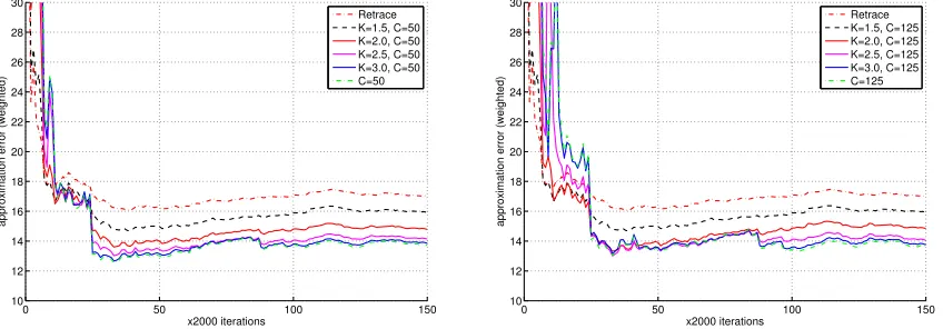
Remark 3.4 (About composite schemes of setting λ) Our motivation for using the composite schemes is revealed by the equation (3.13). Typically each T(i) is designed to be simple to implement in TD learning. For example, if we ignore for now the bounding of traces introduced in Section 2.2 and just consider TD(λ) with constant λ, T(i) can be the Bellman operator T(λ) for TD(λ) with some constant λ. A simple, extreme example is to partition the state space into two sets, and associate one with T(λ), λ = 1, and the other with T(λ), λ = 0. Using the combination (3.13) of the two operators in TD then means that for the first set of states whose λ = 1, we want to estimate their values by using the information about the total rewards received when starting from those states, whereas for the second set of states whose λ= 0, we only use the information about their one-stage rewards and how these states relate to the “neighboring” states in the transition graph. While this way of using different kinds of information for different states is natural and useful for TD-based policy evaluation, it cannot be realized by keeping a single trace sequence as before and only letting λt evolve with states or histories. Indeed, in that case, as discussed in Section 2.2.2, interleaving large and small λt’s would make the algorithm behave effectively like TD with small λover the entire state space.
In the context of the more complex scheme of setting λ discussed in this paper, our motivation and reasons for considering composite schemes are the same. EachT(i) can be designed to be simple to implement, such as in the simple scaling example in Section 2.2. The parameters in theith scheme can be chosen so that they encourage the use of largeλt’s throughout time or dictate the use of only small λt’s. By combining component mappings ofT(i)through (3.13), composite schemes allow us to use cumulative rewards and transition structures at different timescales for different states. This provides additional flexibility in managing the bias-variance trade-off when estimating the value function (see Figure 9 and Figure 11 in Section 4.2.2 for a demonstration).
Finally, we mention that for off-policy LSTD(λ) with constant λ, composite schemes were proposed in (Yu and Bertsekas, 2012) and analyzed in (Yu, 2012, Proposition 4.5, Sec-tion 4.3). Our Corollary 3.1 extends that result. The convergence analysis of the gradient-based algorithms for the composite schemes is given in (Yu, 2017).
3.3 Proofs of Theorem 3.2 and Corollary 3.1
We divide the proof of Theorem 3.2 into two steps. The first step deals with an expression for the trace vector, given in the following lemma. It is more subtle than the other step in the proof, which involves mostly calculations.
We start by extending the stationary state-trace process {(St, yt, et)}t≥0 to t = −1,
−2, . . ., and work with a double-ended stationary process {(St, yt, et)}−∞<t<∞ (by
Recall the shorthand notation (3.1) introduced at the beginning of Section 3: Fork≤m,
ρmk = Qm
i=kρi, λmk = Qm
i=kλi, γmk = Qm
i=kγi, and in addition, λ01 = γ10 = ρ
−1
0 = 1 by convention.
Lemma 3.1 Pζ-almost surely, P∞t=1λ10−tγ10−tρ
−1
−tφ(S−t) is well-defined and finite, and
e0 =φ(S0) +P∞t=1λ01−tγ10−tρ
−1
−tφ(S−t). (3.15)
Proof First, we show Eζ P∞
t=1γ10−tρ−−1t
<∞. Indeed,
Eζ P∞t=1γ10−tρ
−1
−t
=P∞ t=1Eζ
γ10−tρ−−1t
=P∞
t=1ζS>(PΓ)t1<∞,
where the first equality follows from the monotone convergence theorem, the second equality from Condition 2.1(ii) and a direct calculation, and the last inequality follows from Condi-tion 2.1(i) (since (I−PΓ)−1 =P∞
t=0(PΓ)t). This implies P∞
t=1γ10−tρ
−1
−t <∞,Pζ-a.s., so
γ10−tρ−−1t →0 as t→ ∞,Pζ-a.s. Since λ01−t≤1 for allt, it also implies that
Eζ P∞t=1λ10−tγ01−tρ
−1
−tkφ(S−t)k
≤maxs∈Skφ(s)k ·Eζ P∞t=1γ10−tρ
−1
−t
<∞. (3.16)
It then follows from a theorem on integration (Rudin, 1966, Theorem 1.38, p. 28-29) that Pζ-almost surely, the infinite series P∞t=1λ10−tγ10−tρ
−1
−tφ(S−t) converges to a finite limit. We now prove the expression for e0. By unfolding the iteration (2.2) for et backwards in time, we have for all m≥1,
e0 =φ(S0) + Pm−1
t=1 λ01−tγ10−tρ
−1
−tφ(S−t) +λ01−mγ10−mρ
−1
−me−m. (3.17)
Let m → ∞ in the r.h.s. of (3.17). For the last term, the trace e−m lies in a bounded set by Condition 2.3(ii), λ0
1−m ≤1, and as we just showed, γ01−mρ
−1
−m →0, Pζ-a.s. So the last term converges to zeroPζ-a.s. Also as we just showed, the second term convergesPζ-almost surely to P∞
t=1λ01−tγ10−tρ−−1tφ(S−t). The expression (3.15) fore0 then follows.
Proof of Theorem 3.2 Treating λ01 =γ10=ρ−01 = 1, we write the expression ofe0 given in Lemma 3.1 ase0=P∞t=0λ01−tγ10−tρ
−1
−tφ(S−t),Pζ-a.s. We use this expression to calculate first Eζ
e0·ρ0f(S01)
for an arbitrary function f on S × S. (Note that f is bounded and measurable, sinceS is finite.) We have
Eζ
e0·ρ0f(S01)
=P∞ t=0Eζ
h
λ01−tγ10−tρ−−1tφ(S−t)·ρ0f(S01) i
=P∞ t=0Eζ
h
λt1γ1tρt0−1φ(S0)·ρtf(Stt+1) i
=P∞ t=0Eζ
h
φ(S0)·Eζ
λt1γ1tρt0f(Stt+1)|S0, y0, e0 i
(3.18)
where we used the stationarity of the double-ended state-trace process to derive the second equality, and we changed the order of expectation and summation in the first equality. This change is justified by the dominated convergence theorem (cf. (3.16)), and so are similar interchanges of expectation and summation that will appear in the rest of this proof.