Reverse Iterative Volume Sampling for Linear Regression
∗Michał Derezi ´nski [email protected]
Manfred K. Warmuth [email protected]
Department of Computer Science University of California Santa Cruz
Editor:Michael Mahoney
Abstract
We study the following basic machine learning task: Given a fixed set of input points inRdfor a linear regression problem, we wish to predict a hidden response value for each of the points. We can only afford to attain the responses for a small subset of the points that are then used to construct linear predictions for all points in the dataset. The performance of the predictions is evaluated by the total square loss on all responses (the attained as well as the remaining hidden ones). We show that a good approximate solution to this least squares problem can be obtained from just dimensiond
many responses by using a joint sampling technique called volume sampling. Moreover, the least squares solution obtained for the volume sampled subproblem is an unbiased estimator of optimal solution based on allnresponses. This unbiasedness is a desirable property that is not shared by other common subset selection techniques.
Motivated by these basic properties, we develop a theoretical framework for studying volume sampling, resulting in a number of new matrix expectation equalities and statistical guarantees which are of importance not only to least squares regression but also to numerical linear algebra in general. Our methods also lead to a regularized variant of volume sampling, and we propose the first efficient algorithm for volume sampling which makes this technique a practical tool in the machine learning toolbox. Finally, we provide experimental evidence which confirms our theoretical findings. Keywords: volume sampling, linear regression, row sampling, active learning, optimal design
1. Introduction
As an introductory case, consider linear regression in one dimension. We are givennnon-zero points
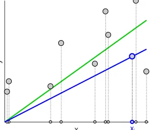
xi. Each point has a hidden real response (or target value)yi. Assume that obtaining the responses is expensive and the learner can afford to request the responsesyifor only a small number of indicesi. After receiving the requested responses, the learner determines an approximate linear least squares solution. In the one dimensional homogeneous case, this is just a single weight. How many response values does the learner need to request so that the total square loss of its approximate solution on allnpoints is “close” to the total loss of the optimal linear least squares solution found with the knowledge of all responses? We will show here that justoneresponse suffices if the indexiis chosen proportional tox2i. When the learner uses the approximate solutionw∗i = yi
xi, then its expected loss equals2times the loss of the optimumw∗that is computed based on all responses (See Figure 1). Moreover, the approximate solutionwi∗is an unbiased estimator for the optimumw∗:
Ei
X
j(xj yi xi
−yj)2
=2 X
j(xjw
∗−
yj)2 and Ei
yi xi
=w∗, whenP(i) ∼ x2i.
∗. This paper is an expanded version of two conference papers (Derezi´nski and Warmuth, 2017, 2018).
c
We will extend these formulas to higher dimensions and to sampling more responses by making use of a joint sampling distribution calledvolume sampling. We next break down our contributions into four parts.
x
y
xi
Figure 1: The expected loss of w∗i = yi
xi
(blue line) based on one responseyiis twice the loss of the optimumw∗(green line). Least squares with dimension many responses. Consider
the case when the pointsxilie inRd. LetXdenote a full rankn×dmatrix that has thentransposed pointsx>i as rows, and lety∈Rnbe the vector of responses. Now the goal is to minimize the (total) square loss,
L(w) =Xn
i=1(x
>
i w−yi)2=kXw−yk2,
over all linear weight vectorsw ∈ Rd. Let w∗ denote the optimal such weight vector. We want to minimize the square loss based on a small number of responses we attained for a subset of rows. Again, the learner is initially given the fixed set ofnrows (i.e. fixed design), but none of the responses. It is then allowed to choose a random
subset of dindices, S ⊆ {1..n}, and obtains the responses for the correspondingdrows. The learner proceeds to find the optimal linear least squares solutionw∗(S)for the subproblem(XS,yS). whereXSis the subset ofdrows ofXindexed byS andyS the correspondingdresponses from the response vector y. As a generalization of the one-dimensional distribution that chooses an index based on the squared length, setSof sizedis chosen proportional to the squared volume of the parallelepiped spanned by the rows ofXS. This squared volume equalsdet(X>SXS). Using elementary linear algebra, we will show thatvolume samplingthe setSassures thatw∗(S)is a good approximation tow∗in the following sense: In expectation, the square loss (on allnrow response pairs) ofw∗(S)is equald+ 1times the square loss ofw∗(whenXis in general position):
E[L(w∗(S))] =(d+ 1)L(w∗), whenP(S)∼det(X>SXS).
Furthermore, we will show that for any sampling procedure that attains less thandresponses, the ratio between the expected loss and the loss of the optimum cannot be bounded by a constant.
Unbiased pseudoinverse estimator. There is a direct connection between solving linear least squares problems and the pseudoinverseX+ of matrixX: For ann−dimensional response vectory, the optimal solution isw∗ = argminw||Xw−y||2 = X+y. Similarlyw∗(S) = (X
S)+yS is the solution for the subproblem(XS,yS). We propose a new implementation of volume sampling calledreverse iterative samplingwhich enables a novel proof technique for obtaining elementary expectation formulas for pseudoinverses based on volume sampling.
x>i
n d
S
XS s
(XS)+
X IS ISX X+ (ISX)+
Suppose that our goal is to estimate the pseudoinverseX+based on the pseudoinverse of a subset of rows. Recall that for a subsetS ⊆ {1..n}ofsrow indices (where the sizesis fixed ands≥d), we letXSbe the submatrix of thesrows indexed byS (see Figure 2). Consider a version ofXin which all but the rows ofSare zero. This matrix equalsISX, where the selection matrixISis an
n-dimensional diagonal matrix with(IS)ii= 1ifi∈Sand 0 otherwise.
For the setSof fixed sizes≥drow indices chosen proportional todet(X>SXS), we can prove the following two expectation formulas (for the second equality,Xmust be in general position):
E[(ISX)+] =X+ and E[ (X>SXS)−1
| {z }
(ISX)+(ISX)+>
] = n−d+ 1 s−d+ 1 (X
>X)−1
| {z }
X+X+> .
Note that(ISX)+has thed×nshape ofX+where thescolumns indexed byScontain(XS)+and the remainingn−scolumns are zero. The expectation of this matrix isX+even though(XS)+is clearly not a submatrix ofX+. This expectation formula now implies that for any sizes≥d, ifS of sizesis drawn by volume sampling, thenw∗(S)is an unbiased estimator1forw∗, i.e.
E[w∗(S)] =E[(XS)+yS] =E[(ISX)+y] =E[(ISX)+]y=X+y=w∗.
The second expectation formula can be viewed as a second moment of the pseudoinverse estimator
(ISX)+, and it can be used to compute a useful notion of matrix variance with applications in random matrix theory:
E[(ISX)+(ISX)+>]−E[(ISX)+]E[(ISX)+]>=
n−s s−d+ 1X
+X+> .
Regularized volume sampling. We also develop a new regularized variant of volume sampling, which extends reverse iterative sampling to selecting subsets of size smaller thand, and leads to a useful extension of the above matrix variance formula. Namely, for anyλ≥0, ourλ-regularized procedure for sampling subsetsSof sizessatisfies
E(X>SXS+λI)−1
n−dλ+ 1
s−dλ+ 1
(X>X+λI)−1,
wheredλ
def
= tr(X(X>X+λI)−1X>)≤dis a standard notion of statistical dimension. Crucially, the above bound holds for subset sizess≥dλ, which can be much smaller than the dimensiond.
Under the additional assumption that response vectoryis generated by a linear transformation distorted with bounded white noise, the expected bound on(X>SXS+λI)−1leads to strong variance bounds for the ridge regression estimator. Specifically, we prove that wheny = Xwe +ξ, with
ξ having mean zero and bounded variance Var[ξ] σ2I, then ifS is sampled according to λ -regularized volume sampling with λ ≤ σ2
kwek
2, we can obtain the following bound on the mean squared prediction error (MSPE):
ESEξ
1 nkX(w
∗
λ(S)−we)k
2
≤ σ 2d
λ
s−dλ+ 1
,
where wλ∗(S) = (X>SXS + λI)−1X>SyS is the ridge regression estimator for the subproblem
(XS,yS). Our new lower bounds show that the above upper bound for regularized volume sampling is essentially optimal with respect to the choice of a subsampling procedure.
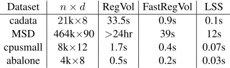
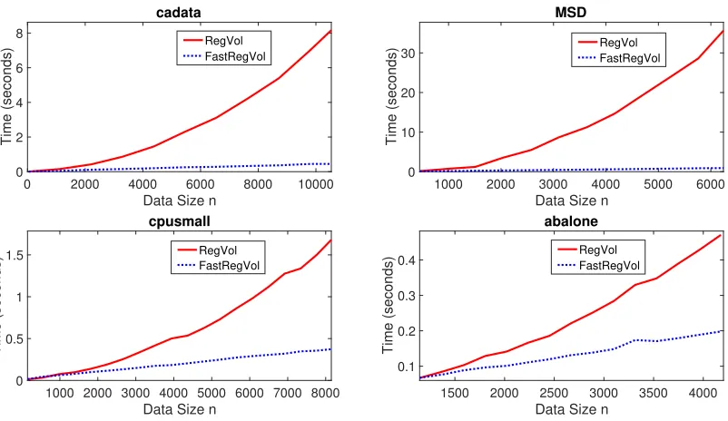
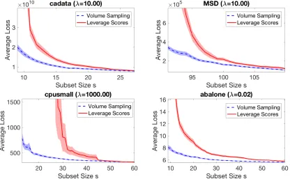
Algorithms and experiments. The only known polynomial time algorithm for sizes > dvolume sampling was recently proposed by Li et al. (2017) with time complexityO(n4s). In this paper we give two new algorithms using our general framework of reverse iterative sampling: one with deterministic runtime ofO((n−s+d)nd), and a second one that with high probability finishes in timeO(nd2). Thus both algorithms improve on the state-of-the-art by a factor of at leastn2 and make volume sampling nearly as efficient as the comparable i.i.d. sampling technique called leverage score sampling. Our experiments on real datasets confirm the efficiency of our algorithms and show that for small sample sizess, volume sampling is more effective than leverage score sampling for the task of subset selection for linear regression.
1.1 Related Work
Volume sampling is a type of determinantal point process (DPP) (Kulesza and Taskar, 2012). DPP’s have been given a lot of attention in the literature with many applications to machine learning, including recommendation systems (Gartrell et al., 2016) and clustering (Kang, 2013). Many exact and approximate methods for efficiently generating samples from this distribution have been proposed (Deshpande and Rademacher, 2010; Kulesza and Taskar, 2011), making it a useful tool in the design of randomized algorithms. Most of those methods focus on samplings≤delements. In this paper, we study volume sampling sets of sizes≥d, which was proposed by Avron and Boutsidis (2013) and motivated with applications in graph theory, linear regression, matrix approximation and more. The problem of selecting a subset of the rows of the input matrix for solving a linear regression task has been extensively studied in statistics literature under the termsoptimal design(Fedorov, 1972) andpool-based active learning(Sugiyama and Nakajima, 2009). Various criteria for subset selection have been proposed, like A-optimality and D-optimality. For example, A-optimality seeks to minimizetr((X>SXS)−1), which is combinatorially hard to optimize exactly. We show that for sizes≥dvolume sampling,E[(X>SXS)−1] = ns−−dd+1+1(X
>X)−1, which provides an approximate
randomized solution of the sampled inverse covariance matrix rather than just its trace.
In the field of computational geometry a variant of volume sampling was used to obtain optimal bounds for low-rank matrix approximation. In this task, the goal is to select a small subset of rows of a matrixX∈Rn×d(much fewer than the rank ofX, which is bounded byd), so that a good low-rank approximation ofXcan be constructed from those rows. Deshpande et al. (2006) showed that volume sampling of sizes < dindex sets obtains optimal multiplicative bounds for this task and polynomial time algorithms for sizes < dvolume sampling were given in Deshpande and Rademacher (2010) and Guruswami and Sinop (2012). We show in this paper that for linear regression, fewer than rank many rows do not suffice to obtain multiplicative bounds. This is why we focus on volume sampling sets of sizes≥d(recall that, for simplicity, we assume thatXis full rank).
2013), but they require all of the responses from the original problem to generate the sketch and are thus not suitable for the goal of using as few response values as possible. The second approach is based on subsampling the rows of the input matrix and only asking for the responses of the sampled rows. The learner optimally solves the sampled subproblem2 and then uses the obtained weight vector for its prediction on all rows. The selected subproblem is known under the term “b-agnostic minimal coreset” in (Boutsidis et al., 2013; Drineas et al., 2008) since it is selected without knowing the response vector (denoted as the vectorb). The second approach coincides with the goals of this paper but the focus here is different in a number of ways. First, we focus on the smallest sample size for which a multiplicative loss bound is possible: Justdvolume sampled rows are sufficient to achieve a multiplicative bound with a fixed factor, whiled−1are not sufficient. A second focus here is the efficiency and the combinatorics of volume sampling. The previous work is mostly based on i.i.d. sampling using the statistical leverage scores (Drineas et al., 2012). As we show in this paper, leverage scores are the marginals of volume sampling and any i.i.d. sampling method requires sample sizeΩ(dlogd)to achieve multiplicative loss bounds for linear regression. On the other hand, the rows obtained from volume sampling areselected jointlyand this makes the chosen subset more informative and brings the required sample size down tod. Third, we focus on the fact that the estimators produced from volume sampling are unbiased and therefore can be averaged to get more accurate estimators. Using our methods, averaging immediately leads to an unbiased estimator with expected loss1 +times the optimum based on samplingd2/responses in total. We leave it as an open problem to construct a1 +factor unbiased estimator from sampling onlyO(d/)responses. If unbiasedness is not a concern, then such an estimator has recently been found (Chen and Price, 2017).
1.2 Outline of the Paper
In the next section, we define volume sampling as an instance of a more general procedure we call reverse iterative sampling, and we use this methodology to prove closed form matrix expressions for the expectation of the pseudoinverse estimator(ISX)+and its square(ISX)+(ISX)+>, when
S is sampled by volume sampling. Central to volume sampling is the Cauchy-Binet formula for determinants. As a side, we produce a number of short self-contained proofs for this formula and show that leverage scores are the marginals of volume sampling. Then in Section 3 we formulate the problem of solving linear regression from a small number of responses, and state the upper bound for the expected square loss of the volume sampled least squares estimator (Theorem 8), followed by a discussion and related lower bounds. In Section 3.3, we prove Theorem 8 and an additional related matrix expectation formula. We next discuss in Section 3.4 how unbiased estimators can easily be averaged for improving the expected loss and discuss open problems for constructing unbiased estimators. A new regularized variant of volume sampling is proposed in Section 4, along with the statistical guarantees it offers for computing subsampled ridge regression estimators. Next, we present efficient volume sampling algorithms in Section 5, based on the reverse iterative sampling paradigm, which are then experimentally evaluated in Section 6. Finally, Section 7 concludes the paper by suggesting a future research direction.
2. Reverse Iterative Sampling
Letnbe an integer dimension. For each subsetS ⊆ {1..n}of sizeswe are given a matrix formula
F(S). Our goal is to sample setSof sizesusing some sampling process and then develop concise expressions forES:|S|=s[F(S)]. Examples of formula classesF(S)will be given below.
{1..n}
S
S−i P(S−i|S)
size
n
n−1
s s
s−1
d
Figure 3:Reverse iterative sampling.
We represent the sampling by a directed acyclic graph (DAG), with a single root node corresponding to the full set {1..n}. Starting from the root, we proceed along the edges of the graph, iteratively removing elements from the setS(see Figure 3). Concretely, consider a DAG with levels
s = n, n−1, ..., d. Level s contains ns
nodes for sets
S ⊆ {1..n}of sizes. Every node S at levels > d has s
directed edges to the nodesS− {i}(also denotedS−i) at the next lower level. These edges are labeled with a conditional probability vectorP(S−i|S), where the eventSoccurs if the sampling process visits nodeSas it traces a (directed) path in the DAG from the root node{1..n}to a node at leveld. Such paths haven−dedges. It is natural to assign probabilities
to shorter paths as well going from any node to a node at a lower level. The probability of such a path is again the product of its edge probabilities. It also follows that the probabilityP(S)of visiting nodeS(via a path from the root) is the sum of the probabilities of all paths from root toS. Finally, the probabilityP({1..n})of the root node is 1 and more generally, the total probability of all nodes at each layer is 1.
We associate a formulaF(S)with each set nodeSin the DAG. The following key equality lets us compute expectations.
Lemma 1 If for allS⊆ {1..n}of size greater thandwe have
F(S) =X
i∈S
P(S−i|S)F(S−i),
then for anys∈ {d..n}: ES:|S|=s[F(S)] =
P
S:|S|=sP(S)F(S) =F({1..n}).
Proof Suffices to show that expectations at successive layerssands−1are equal fors > d:
X
S:|S|=s
P(S)F(S)= X
S:|S|=s
P(S)X
i∈S
P(S−i|S)F(S−i)=
X
S:|S|=s
X
i∈S
P(S)P(S−i|S)F(S−i)
= X
T:|T|=s−1
X
j /∈T
P(T+j)P(T|T+j)
| {z }
P(T)
F(T).
2.1 Volume Sampling
Given a tall full rank matrixX∈ Rn×dand a sample sizes∈ {d..n}, volume sampling chooses subsetS ⊆ {1..n}of sizeswith probability proportional to squared volume spanned by the columns of submatrix3 XS and this squared volume equalsdet(X>SXS). The following theorem uses the above DAG setup to compute the normalization constant for this distribution. Note that all subsetsS
of volume 0 will be ignored, since they are unreachable in the proposed sampling procedure.
Theorem 2 LetX ∈ Rn×d, whered ≤ nanddet(X>X) > 0. For any setS of sizes > d for
whichdet(X>SXS)>0, define the probability of the edge fromStoS−ifori∈Sas:
P(S−i|S)
def
= det(X >
S−iXS−i) (s−d)det(X>SXS)
=1−x >
i (X>SXS)−1xi
s−d , (reverse iterative volume sampling)
where x>i is thei-th row of X. In this case P(S−i|S) is a proper probability distribution. If
det(X>SXS) = 0, then simply setP(S−i|S)to1s. With these definitions,PS:|S|=sP(S) = 1for all
s∈ {d..n}and the probability of all paths from the root to any subsetSof size at leastdis
P(S) = det(X >
SXS) n−d
s−d
det(X>X). (volume sampling)
The rewrite of the ratio det(X
>
S−iXS−i)
det(X>SXS) as1−x >
i (X>SXS)−1xiis Sylvester’s Theorem for determi-nants. Incidentally, this is the only property of determinants used in this section.
The theorem also implies a generalization of the Cauchy-Binet formula to sizes≥dsets:
X
S:|S|=s
det(X>SXS) =
n−d s−d
det(X>X). (1)
Whens= d, then the binomial coefficient is 1 and the above becomes the vanilla Cauchy-Binet formula. The below proof of the theorem thus results in a minimalist proof of this classical formula as well. The proof uses the reverse iterative sampling (Figure 3) and the fact that all paths from the root to nodeShave the same probability. For the sake of completeness we also give a more direct inductive proof of the above generalized Cauchy-Binet formula in Appendix A.
Proof First, for any nodeSs.t.s > danddet(XS>XS)>0, the probabilities out ofSsum to 1:
X
i∈S
P(S−i|S) =
X
i∈S
1−tr((X>SXS)−1xix>i )
s−d =
s−tr((X>SXS)−1X>SXS)
s−d =
s−d s−d = 1.
It remains to show the formula for the probability P(S) of all paths ending at node S. If
det(X>SXS) = 0, then one edge on any path from the root toShas probability 0. This edge goes from a superset ofSwith positive volume to a superset ofSthat has volume 0. Since all paths have probability 0,P(S) = 0in this case.
Now assumedet(X>SXS) > 0and consider any path from the root {1..n} toS. There are
(n−s)!such paths all going through sets with positive volume. The fractions of determinants in the
probabilities along each path telescope and the additional factors accumulate to the same product. So the probability of all paths from the root toSis the same and the total probability intoSis
(n−s)! (n−d). . .(s−d+ 1)
det(X>SXS)
det(X>X) = 1 n−d s−d
det(X>SXS)
det(X>X) .
An immediate consequence of the above sampling procedure is the following composition property of volume sampling, which states that this distribution is closed under subsampling. We also give a direct proof to highlight the combinatorics of volume sampling.
Corollary 3 For anyX∈Rn×dandn≥t > s≥d, the following hierarchical sampling procedure:
T ∼t X (sizetvolume sampling fromX), S ∼s XT (sizesvolume sampling fromXT)
returns a setSwhich is distributed according to sizesvolume sampling fromX.
Proof We start with the Law of Total Probability and then use the probability formula for volume sampling from the above theorem. HereP(T ∩S)means the probability of all paths going through nodeT at leveltand ending up at the final nodeSat levels. IfS6⊆T, thenP(T ∩S) = 0.
P(S) = X
T:S⊆T
P(T∩S)
z }| {
P(S|T) P(T)
= X
T:S⊆T
det(X>SXS)
t−d s−d
det(X>TXT)
det(X>TXT)
n−d t−d
det(X>X)
=
n−s t−s
det(X>SXS)
t−d s−d
n−d t−d
det(X>X) =
det(X>SXS)
n−d s−d
det(X>X).
Note that for all setsT containingS, the probabilityP(T ∩S)is the same, and there are nt−−sssuch sets.
The main competitor of volume sampling is i.i.d. sampling of the rows ofXw.r.t. the statistical leverage scores. For an input matrixX∈Rn×d, the leverage score of thei-th rowx>
i ofXis defined as
li
def
=x>i (X>X)−1xi.
Recall that this quantity appeared in the definition of conditional probabilityP(S−i|S)in Theorem 2, where the leverage score was computed w.r.t. the submatrixXS. In fact, there is a more basic relationship between leverage scores and volume sampling: If setS is sampled according to size
Proposition 4 Let X ∈ Rn×dbe a full rank matrix and s ∈ {d..n}. IfS ⊆ {1..n} is sampled according to sizesvolume sampling, then for anyi∈ {1..n},
P(i∈S) = s−d n−d+
n−s n−d
li
z }| {
x>i (X>X)−1xi.
Proof Instead ofP(i∈S)we will first computeP(i /∈S):
P(i /∈S) = X
S:|S|=s,i /∈S
det(X>SXS) n−d
s−d
det(X>X)
= X
S:|S|=s,i /∈S
P
T⊆S:|T|=ddet(X
>
TXT) n−d
s−d
det(X>X)
=
n−d−1
s−d
det(X> −iX−i)
z }| {
X
T:|T|=d,i /∈T
det((X−i)>T(X−i)T)
n−d s−d
det(X>X)
= n−s
n−d 1−x >
i (X>X)−1xi
,
where we used Cauchy-Binet twice and the fact that every set T : |T|=d, i /∈ T appears in n−d−1
s−d
sets S : |S| = s, i /∈ S. Now, the marginal probability follows from the fact that
P(i∈S) = 1−P(i /∈S).
2.2 Expectation Formulas for Volume Sampling
All expectations in the remainder of the paper are w.r.t. volume sampling. We use the short-hand E[F(S)]for expectation with volume sampling where the size of the sampled set is fixed tos. The expectation formulas for two choices ofF(S)are proven in Theorems 5 and 6. By Lemma 1 it suffices to showF(S) =P
i∈SP(S−i|S)F(S−i)for volume sampling. We also present a related expectation formula (Theorem 7), which is proven later using different techniques.
Recall thatXSis the submatrix of rows indexed byS ⊆ {1..n}. We also use a version ofXin which all but the rows ofSare zeroed out. This matrix equalsISXwhereISis ann-dimensional diagonal matrix with(IS)ii= 1ifi∈Sand 0 otherwise (see Figure 2).
Theorem 5 LetX ∈Rn×dbe a tall full rank matrix (i.e. n≥d). Fors∈ {d..n}, letS ⊆ {1..n} be a sizesvolume sampled set overX. Then
E[(ISX)+] =X+.
For the special case ofs = d, this fact was known in the linear algebra literature (Ben-Tal and Teboulle, 1990; Ben-Israel, 1992). It was shown there using elementary properties of the determinant such as Cramer’s rule.4 The proof methodology developed here based on reverse iterative volume
sampling is very different. We believe that this fundamental formula lies at the core of why volume sampling is important in many applications. In this work, we focus on its application to linear regression. However, Avron and Boutsidis (2013) discuss many problems where controlling the pseudoinverse of a submatrix is essential. For those applications, it is important to establish variance bounds for the above expectation and volume sampling once again offers very concrete guarantees. We obtain them by showing the following formula, which can be viewed as a second moment for this estimator.
Theorem 6 LetX∈Rn×dbe a full rank matrix ands∈ {d..n}. If sizesvolume sampling overX has full support, then
E[ (X>SXS)−1
| {z }
(ISX)+(ISX)+>
] = n−d+ 1 s−d+ 1 (X
>X)−1
| {z }
X+X+> .
In the case when volume sampling does not have full support, then the matrix equality “=” above is replaced by the positive-definite inequality “”.
The condition that sizesvolume sampling overXhas full support is equivalent todet(X>SXS)>0 for allS ⊆ {1..n}of sizes. Note that if sizesvolume sampling has full support, then sizet > s
also has full support. So full support for the smallest sized(often phrased asXbeingin general position) implies that volume sampling w.r.t. any sizes≥dhas full support.
The above theorem immediately gives an expectation formula for the Frobenius normk(ISX)+kF of the estimator:
Ek(ISX)+k2F
=E[tr((ISX)+(ISX)+>)] =
n−d+ 1 s−d+ 1kX
+k2
F. (2)
This norm formula was shown by Avron and Boutsidis (2013), with numerous applications. Theorem 6 can be viewed as a much stronger pre-trace version of the known norm formula. Also our proof techniques are quite different and much simpler. Note that if sizesvolume sampling forXdoes not have full support, then (2) becomes an inequality.
We now mention a second application of the above theorem in the context of linear regression for the case when the response vectoryis modeled as a noisy linear transformation, i.e.,y=Xwe +ξ for somewe ∈ R
dand a random noise vectorξ ∈
Rn (detailed discussion in Section 4). In this case the matrix(X>SXS)−1can be interpreted as the covariance matrix of least-squares estimator
w∗(S)(for a fixed setS) and Theorem 6 gives an exact formula for the covariance matrix ofw∗(S)
under volume sampling. In Section 4, we give an extended version of this result which provides even stronger guarantees for regularized least-squares estimators under this model (Theorem 16).
Note that except for the above application, all results in this paper hold for arbitrary response vectorsy. By combining Theorems 5 and 6, we can also obtain a covariance-type formula5for the pseudoinverse matrix estimator:
E[((ISX)+−E[(ISX)+]) ((ISX)+−E[(ISX)+])>]
=E[(ISX)+(ISX)+>]−E[(ISX)+]E[(ISX)+]>
= n−d+ 1 s−d+ 1 X
+X+>−X+X+>= n−s s−d+ 1 X
+X+>. (3)
We now give the background for a third matrix expectation formula for volume sampling. Pseudoinverses can be used to compute the projection matrix onto the span of columns of matrixX, which is defined as follows:
PX
def
=X
X+
z }| {
(X>X)−1X>.
Applying Theorem 5 leads us immediately to the following unbiased matrix estimator for the projection matrix:
E[X(ISX)+] =XE[(ISX)+] =XX+=PX.
Note that this matrix estimatorX(ISX)+is closely connected to linear regression: It can be used to transform the response vectoryinto the prediction vectoryb(S)of subsampled least squares solution
w∗(S)as follows:
b
y(S) =X(ISX)+y
| {z }
w∗(S) .
In this case, volume sampling once again provides a covariance-type matrix expectation formula.
Theorem 7 LetX∈Rn×dbe a full rank matrix. If matrixXis in general position andS⊆ {1..n} is sampled according to sizedvolume sampling, then
E[ (X(ISX)+)2
| {z }
(ISX)+>X>X(ISX)+
]−PX=d(I−PX).
IfXis not in general position, then the matrix equality “=” is replaced by the positive-definite inequality “”.
Note that this third expectation formula is limited to sample sizes=d. It is a direct consequence of Theorem 8 given in the next section which relates the expected loss of a subsampled least squares estimator to the loss of the optimum least squares estimator. Unlike the first two formulas given in theorems 5 and 6, its proof does not rely on the methodology of Lemma 1, i.e., on showing that the expectations at all levels of a certain DAG associated with the sampling process are the same. We defer the proof of this third expectation formula to the end of Section 3.3. No extension of this third formula to sample sizes > dis known.
Proof of Theorem 5 We apply Lemma 1 withF(S) = (ISX)+. It suffices to show F(S) =
P
i∈SP(S−i|S)F(S−i)forP(S−i|S) = 1−x>
i (X>SXS)−1xi
s−d , i.e.:
(ISX)+=
X
i∈S
1−x>i (X>SXS)−1xi
s−d (IS−iX)
+
| {z }
(X>S
−iXS−i)−1(IS−iX)>
.
We first apply Sherman-Morrison to (X>S−iXS−i)
−1 = (X>
SXS−xix
>
i )−1 on the r.h.s. of the above:
X
i
1−x>i (X>SXS)−1xi
s−d
(X>SXS)−1+
(X>SXS)−1xix>i (X>SXS)
−1
1−x>i (X>SXS)−1xi
Next we expand the last two factors into 4 terms. The expectation of the first(X>SXS)−1(ISX)>is
(ISX)+(which is the l.h.s.) and the expectations of the remaining three terms timess−dsum to 0:
−X i∈S
(1−x>i (XS>XS)−1xi) (X>SXS)−1xie>i + (X>SXS)−1
X
i∈S
xix>i (X>SXS)−1(ISX)>
−X i∈S
(X>SXS)−1xi (x>i (X>SXS)−1xi)e>i = 0.
In Appendix B we give an alternate proof using a derivative argument.
Proof of Theorem 6 ChooseF(S) = ns−−dd+1+1(X>SXS)−1. By Lemma 1 it suffices to showF(S) =
P
i∈SP(S−i|S)F(S−i)for volume sampling:
s−d+ 1
((((
( n−d+ 1(X
>
SXS)−1 =
X
i∈S
1−x>i (X>SXS)−1xi
s−d
s−d
((((
( n−d+ 1(X
>
S−iXS−i) −1.
To show this we apply Sherman-Morrison to(X>S−iXS−i)
−1on the r.h.s.:
X
i∈S
(1−x>i (XS>XS)−1xi)
(X>SXS)−1+
(X>SXS)−1xix>i (X>SXS)−1
1−x>i (X>SXS)−1xi
=(s−d)(X>SXS)−1+
(X>SXS)−1
X
i∈S
xix>i (X
>
SXS)−1 = (s−d+ 1) (X>SXS)−1.
If some denominators1−x>i (X>SXS)−1xiare zero, then we only sum overifor which the denomi-nators are positive. In this case the above matrix equality becomes a positive-definite inequality.
3. Linear Regression with Smallest Number of Responses
Our main motivation for studying volume sampling came from asking the following simple question. Suppose we want to solve ad-dimensional linear regression problem with an input matrixXofn
rows inRdand a response vectory ∈Rn, i.e. findw∈Rdthat minimizes the least squares loss kXw−yk2on allnrows. We useL(w)to denote this loss. The optimal weight vector minimizes
L(w), i.e.
w∗= argmindef
w∈Rd
L(w) =X+y.
Computing it requires access to the input matrixX and the response vectory. Assume we are givenXbut the access to response vectoryis restricted. We are allowed to pick a random subset
S ⊆ {1..n}of fixed sizesfor which the responsesySfor the submatrixXSare revealed to us, and then must produce a weight vectorw(X, S,yS) ∈Rdfrom a subset of row indicesSof the input matrixXand the corresponding responsesyS. Our goal in this paper is to find a distribution on the subsetsSof sizesand aweight functionw(X, S,yS)s.t.6
∀(X,y)∈Rn×d×Rn×1: E[L(w(X, S,yS))]≤(1 +c)L(w∗),
6. Since the learner is givenX, it is natural to define the optimal multiplicative constant specialized for eachX:
wherecmust be a fixed constant (that is independent ofXandy). Throughout the paper we use the one argument shorthandw(S)for the weight functionw(X, S,yS). We assume that attaining response values is expensive and ask the question: What is the smallest number of responses (i.e. smallest size ofS) for which such a multiplicative bound is possible? We will use volume sampling to show that attainingdresponse values is sufficient and show that less thandresponses is not.
L(·)
L(w∗) E[L(w∗(S))]
L(w∗(Si))
L(w∗(Sj))
w∗(Si) w∗=E[w∗(S)] w∗(Sj) d L(w∗)
Figure 4:Unbiased estimatorw∗(S)in expecta-tion suffers loss(d+ 1)L(w∗).
Before we state our main upper bound based on volume sampling, we make the following key obser-vation: If for the subproblem (XS,yS) there is a weight vector w(S) that has loss zero, then the al-gorithm has to predict with such a consistent weight vector. This is because in that case the responsesyS can be extended to a response vectoryfor all ofXs.t.
L(w∗) = 0. Thus since we aim for a multiplicative loss bound, we force the algorithm to predict with the optimum solutionw∗(S)= (def XS)+ySwhenever the subproblem(XS,yS)has loss 0. In particular, when |S|=dandXShas full rank, then there is a unique consistent solutionw∗(S)for the subproblem and the learner must use the weight functionw(S) =w∗(S).
Theorem 8 If the input matrix X ∈ Rn×d is in general position, then for any response vector
y ∈ Rn, the expected square loss (on alln rows of X) of the optimal solution w∗(S) for the
subproblem(XS,yS), with thed-element setSobtained from volume sampling, is given by
E[L(w∗(S))] = (d+ 1)L(w∗).
IfXis not in general position, then the expected loss is upper-bounded by(d+ 1)L(w∗).
There are no range restrictions on thenpoints and response values in this bound. Also, as discussed in the introduction, this bound is already non-obvious for dimension 1, when the multiplicative factor is 2 (See Figure 1 for a visualization). Note that if there is a bias term in dimension 1, then the factor becomes 3.
In dimensiond, it is instructive to look at the case when the square loss of the optimum solution is zero, i.e. there is a weight vectorw∗∈Rds.t.Xw∗ =y. In this case the response values of anyd linearly independent rows ofXdetermine the optimum solution and the multiplicative loss formula of the theorem clearly holds. The formula specifies how noise-free case generalizes gracefully to the noisy case in that for volume sampling, the expected square loss of the solution obtained fromd
row response pairs is always by a factor of at mostd+ 1larger than the square loss of the optimum solution. Moreover, sinceE[w∗(S)] =w∗and the loss functionL(·)is convex, we have by Jensen’s inequality that
EL(w∗(S))≥L E[w∗(S)]=L(w∗).
The above theorem now states that the gap E[L(w∗(S))]−L(w∗) in Jensen’s inequality (which coincides with the “regret” of the estimator) equalsd L(w∗), when the expectation is w.r.t. sized
EL(w∗(S))−L( E[w∗(S)]
z}|{ w∗ )
| {z }
regret
= d L(w∗)
| {z }
gap in Jensen’s
=EkXw∗(S)−Xw∗k2
| {z }
variance
.
We now make a number of observations and present some lower bounds that highlight the upper bound of the above theorem. Then, in Section 3.3 we prove the theorem and a matrix expectation formula implied by it.
3.1 WhenXis not in General Position
The above theorem gives an equality for the expected loss of a volume-sampled solution. However, this equality is only guaranteed to hold when matrixXis in general position. We give a minimal example problem where the matrixXis not in general position and the equality of Theorem 8 turns into a strict inequality. This shows that for the equality, the general position assumption is necessary. If we apply even an infinitesimal additive perturbation to the matrixXof the example problem, then the resulting matrixXis in general position and the equality holds. Note that even though the optimum lossL(w∗)does not change significantly under such a perturbation, the expected sampling lossE[L(w∗(S))]has to jump sufficiently to close the gap in the inequality. In our minimal example problem,n= 3andd= 2, and
X=
1 1
1 1
1 0
, y=
1 0 0
.
We have three 2-element subsets to sample from: S1 ={1,2}, S2 ={2,3}, S3 ={1,3}.Notice that the first two rows ofXare identical, which means that the probability of sampling setS1 is 0 in the volume sampling process. The other two subsets,S2andS3, form identical submatrices
XS2 = XS3. Therefore they are equally probable. The optimal weight vectors for these sets are
w∗(S2)= (0,0)>andw∗(S3)= (0,1)>. Alsow∗ = (0,12)>and the expected loss is bounded as:
E[L(w∗(S))] = 1 2
1
z }| {
L(w∗(S2)) + 1 2
1
z }| {
L(w∗(S3))
| {z }
1
<
3
z }| {
(d+ 1)
1/2
z }| {
L(w∗)
| {z }
3/2
.
Now consider a slightly perturbed input matrix
X =
1 1 +
1 1
1 0
,
where >0is arbitrarily small (We keep the response vectorythe same). Now, there is nod×d
submatrix that is singular, so the upper bound from Theorem 8 must be tight. The reason is that even though subset S1 still has very small probability, its loss is very large, so the expectation is significantly affected by this component, no matter how smallis. We see this directly in the calculations. Letw∗andw∗(Si)be the corresponding solutions for the perturbed problem and its
subproblems. The volumes of the subproblems and their losses are:
det(X>S1XS1) =2 L(w∗(S1)) =−2 det(X>S2XS2) = 1 L(w∗(S2)) = 1
det(X>S3XS3) = (1 +)2 L(w∗(S3)) = (1 +)−2
Note that for each subproblem, the product of volume times loss is equal to 1. Now the expected loss can be easily computed, and we can see that the gap in the bound disappears (the denominator is the normalizing constant for volume sampling):
E[L(w∗(S))] = 1 + 1 + 1
2+ 1 + (1 +)2 = (d+ 1)L(w
∗).
3.2 Lower Bounds and the Importance of Joint Sampling
The factord+ 1in Theorem 8 cannot, in general, be improved when selecting onlydresponses:
Proposition 9 For anyd, there exists a least squares problem(X,y)withd+ 1rows inRdsuch that for everyd-element index setS ⊆ {1.. d+1}, we have
L(w∗(S)) = (d+ 1)L(w∗).
Proof Choose the input vectorsxi(and rowsx>i ) as thed+ 1corners of any simplex inRdcentered at the origin and choose alld+ 1responses as the same non-zero valueα. For anyα, the optimal solutionw∗will be the all-zeros vector with loss
L(w∗) = (d+ 1)α2.
On the other hand, taking any sizedsubset of indicesS ⊆ {1.. d+1}, the subproblem solution
w∗(S)will only produce loss on the left out input vector xi, indexed withi 6∈ S. To obtain the prediction onxi, we use a simple geometric argument. Observe that since the simplex is centered, we can write the origin ofRdin terms of the corners of the simplex as
0=X
k
xk=xi+dx¯−i, wherex¯−i
def
= 1 d
X
k6=i
xk.
Thus, the left out input vectorxiequals−dx¯−i. The prediction ofw∗(S)on this vector is
b
yi=x>i w
∗
(S)=−d
1 d
X
k6=i
x>k
w∗(S)=−X k6=i
x>kw∗(S)=−dα.
It follows that the loss ofw∗(S)equals
L(w∗(S)) = (ybi−yi)2 = (−dα−α)2 = (d+ 1)2α2 = (d+ 1)L(w∗).
Moreover, it is easy to show that nodeterministicalgorithm for selectingdrows (without knowing the responses) can guarantee a multiplicative loss bound with a factor less thann/d(Boutsidis et al., 2013). For the sake of completeness, we show this here ford= 1:
Proposition 10 For anyn×1input matrixXof all 1’s and any deterministic algorithm that chooses some singleton setS ={i}, there is a response vectoryfor which the loss of the subproblem and the optimal loss are related as follows:
Proof If the response vectoryis the vector ofn1’s except for a single 0 at indexi, then we have
L(
0
z }| {
w∗({i})
| {z }
n−1
) =n L(
n−1
n
z}|{ w∗)
| {z }
n−1
n .
Note that for the 1-dimensional example used in the proof, volume sampling would pick the setS uniformly. For this distribution, the multiplicative factor drops from ndown to 2, that is E[L(w∗(S))] = n1(n−1) +n−n11 = 2L(w∗).
The importance of joint sampling. Three properties of volume sampling play a crucial role in achieving a multiplicative loss bound:
a) Randomness.No deterministic algorithm guarantees such a bound (see Proposition 10).
b) The chosen submatrices must have full rank. Choosing any rank deficient submatrix with positive probability, does not allow for a multiplicative bound (see Propositions 11 and 12).
c) Jointness. No i.i.d. sampling procedure can achieve a multiplicative loss bound withO(d)
responses (see Corollary 13).
By jointly selecting subsetS, volume sampling ensures that the corresponding input vectorsxi are well spread out in the input spaceRd. In particular, volume sampling does not put any probability mass on setsSsuch that the rank of submatrixXSis less thand. Intuitively, selecting rank deficient row subsets should not be effective, since such a choice leads to an under-determined least squares problem. We make this simple statement more precise by showing that any randomized algorithm, that with positive probability selects a rank deficient row subset, cannot achieve a multiplicative loss bound. Intuitively if the algorithm picks a rank deficient subset then it is not clear how it should select the weight vectorw(S)given input matrixX, subsetSand responsesyS. We reasoned before that
w(S)must have loss 0 on the subproblem(XS,yS). However ifrank(XS)< d, then the choice of the weight vectorw(S)with loss 0 is not unique and this causes positive loss for some response vectory.
Proposition 11 If for any input matrixX, the algorithm samples a rank deficient subsetSof rows with positive probability, then the expected loss of the algorithm cannot be bounded by a constant times the optimum loss for all response vectorsy.
Note that this means in particular that ifXhas rankd, then samplingd−1size subsets with positive probability does not allow for a constant factor approximation.
Proof LetSbe a rank deficient subset chosen with probabilityP(S) >0. Since in our setup the bound has to hold for all response vectorsywe can imagine an adversary choosing a worst-case
y. This adversary gives all rows ofXSthe response value zero. Letw(S)be the plane produced by the algorithm when choosing S and receiving the responses 0 for XS. Let i ∈ {1..n} s.t.
We now strengthen the above proposition in that whenever the sampleSis rank deficient then the loss of the optimum is zero while the loss of the algorithm is positive. However note that this proposition is weaker than the above in that it only holds for specific input matrices.
Proposition 12 Letd≤nand letXbe any input matrix of rankdconsisting ofnstandard basis row vectors inRd. Then for any randomized learning algorithm that with probabilitypselects a subsetSs.t.rank(XS)< dand any weight functionw(·), there is a response vectory, satisfying:
L(w∗) = 0, and L(w(S))>0 with probability at leastp.
Proof Let Q = {1,2, . . . ,2n}. The adversarial response vector y is constructed by carefully selecting one of the weight vectorsw∗∈Qd, and setting the response vectorytoXw∗. This ensures thatL(w∗) = 0and sinceXconsists of standard basis row vectors, the components ofylie inQas well. Note that if the learner does not discoverw∗exactly, it will incur positive loss. LetHbe the set of all rank deficient sets inX, i.e. those that lack at least one of the standard basis vectors:
H={S⊆ {1..n} : rank(XS)< d}.
Suppose that given matrixX, the learner uses weight functionw(S,yS). (Note that for the sake of concreteness we stopped using the single argument shorthand for the weight function during this proof.) We will count the number of possible inputs to this function, whenSis a rank deficient index set of the rows ofXand the response vectoryS is consistent with somew∗ ∈ Qd. For any fixed rank deficient setS, lettbe the number of distinct basis vectors appearing inXS. Clearlyt≤d−1. Fix a subsetT ⊆Sof sizets.t.XT contains alltbasis vectors ofXSexactly once (Thus the basis vectors inXS\T are all duplicates). Sincey∈Qn, the components ofySalso lie inQandyS is determined by the responses ofyT. Clearly there are at most|Q|d−1choices foryT. It follows that the number of possible input pairs(S,yS)for functionw(·,·)under the above restrictions can be bounded as
n
(S,yS) : [S ∈H]and[yS =XSw∗forw∗ ∈Qd]
o
≤ |H|
|{z}
<2n max
S∈H|{XSw ∗
: w∗∈Qd}|
| {z }
≤|Q|d−1
<2n|Q|d−1 =|Qd|.
So for every weight functionw(·,·), there existsw∗ ∈Qdthat is not present in the set{w(S,yS) :
S ∈H}. Selectingy=Xw∗for the adversarial response vector, we guarantee that the learner picks the wrong solution for every rank deficient setSand therefore receives positive loss w.p. at leastp.
Using Proposition 12, we show that any i.i.d. row sampling distribution (like for example leverage score sampling) requiresΩ(dlogd)samples to get any multiplicative loss bound, either with high probability or in expectation.
Corollary 13 Letd≤ nand letXbe any input matrix of rank dconsisting ofnstandard basis row vectors inRd. Then for any randomized learning algorithm which selects a random multiset
S ⊆ {1..n}of size|S| ≤(d−1) ln(d)via i.i.d. sampling from any distribution and uses any weight functionw(S), there is a response vectorysatisfying:
Proof Any i.i.d. sample of size at most(d−1) ln(d)with probability at least1/2does not contain all of the unique standard basis vectors (Coupon Collector Problem7). Thus, with probability at least
1/2submatrixXS has rank less thand. Now, for any such algorithm we can use Proposition 12 to select a consistent adversarial response vectorysuch that with probability at least1/2the loss
L(w(S))is positive.
Note that the corollary requiresXto be of a restricted form that contains a lot of duplicate rows. It is open whether this corollary still holds whenXis an arbitrary full rank matrix.
3.3 Proof of the Loss Expectation Formula
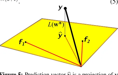
First, we discuss several key connections between linear regression and volume, which are used in the proof. Note that the lossL(w∗) suffered by the optimum weight vector can be written as kyb−yk2, the squared Euclidean distance between prediction vector
b
y=Xw∗and the response vectory. Sinceyb is minimizing the distance fromyto the subspace ofR
nspanning the feature vectors{f1, . . . ,fd}(columns ofX), it has to be theprojectionofyonto that subspace (see Figure 5). We denote this projection asPXy, as defined in Section 2.2. Note thatPXis a linear mapping fromRnonto the column span of the matrixXsuch that
foru∈span(X) u=PXy ⇔ PX(u−y) =0 ⇔ X>(u−y) =0. (4)
We next give a second geometric interpretation of the lengthkby−yk2. LetPbe the parallelepiped formed by thedcolumn/feature vectors of the input matrixX. Furthermore, consider the extended input matrix produced by adding the response vectorytoXas an extra column:
e
X= (def X,y)∈Rn×(d+1). (5)
y
y
f1 f2
L(w*)
Figure 5:Prediction vectorybis a projection ofy onto the span of feature vectorsfi.
Using the “base×height” formula we can relate the volume ofPto the volume ofP, the parallelepipede
formed by thed+ 1columns ofXe. Observe thatPe
hasPas one of its faces, with the response vectory
representing the edge that protrudes from that face. Hence the volume ofePis the product of the volume
ofPand the distance betweenyand span(X). This distance equalskby−yk, since as discussed above,yb
is the projection ofyonto span(X). Thus we have
det(Xe>Xe) = det(X>X)L(w∗). (6)
Next, we present a proposition whose corollary is key to proving Theorem 8. Suppose that we select one test row from the input matrix and use the remainingn−1row response pairs as the training set. The proposition relates the loss of the obtained solution on the test row to the total leave-one-out loss an all rows.
Proposition 14 For any indexi∈ {1..n}, letw∗(−i)be the solution to the reduced linear regression problem(X−i,y−i). Then
L(w∗(−i))−L(w∗) =
det(X>X)−det(X>−iX−i) det(X>X)
z }| {
x>i (X>X)−1xi `i(w∗(−i)), where`i(w)
def
= (x>i w−yi)2is the square loss ofwon thei-th point.
An algebraic proof of this proposition essentially appears in the proof of Theorem 11.7 in Cesa-Bianchi and Lugosi (2006). For the sake of completeness we give a new geometric proof of this proposition in Appendix C using basic properties of volume, thus stressing the connection to volume sampling.
Note that if matrixXhas exactlyn=d+ 1rows and the training matrixX−iis full rank, then
w∗(−i)has loss zero on all training rows. In this case we obtain a simpler relationship than the proposition.
Corollary 15 IfXhasd+ 1rows andrank(X−i) =d, then definingXe as in (5), we have
det(Xe>Xe) = det(X>−iX−i)`i(w∗(−i)).
Proof By Proposition 14 and the fact thatL(w∗(−i)) =`i(w∗(−i)), we have
det(X>X)L(w∗) = det(X>−iX−i)`i(w∗(−i)). The corollary now follows from the “base×height” formula for volume.
We are now ready to present the proof of Theorem 8. Recall that our goal is to find the expected lossE[L(w∗(S))], whereSis a sizedvolume sampled set.
Proof of Theorem 8 First, we rewrite the expectation as follows:
E[L(w∗(S))] = X
S,|S|=d
P(S)L(w∗(S)) = X
S,|S|=d
P(S)
n
X
j=1
`j(w∗(S))
= X
S,|S|=d
X
j /∈S
P(S)`j(w∗(S)) =
X
T,|T|=d+1
X
j∈T
P(T−j)`j(w∗(T−j)). (7)
We now use Corollary 15 on the matrixXT and test rowx>j (assumingrank(XT−j) =d):
P(T−j)`j(w∗(T−j)) =
det(X>T−jXT−j) det(X>X) `j(w
∗
(T−j)) =
det(Xe>TXeT)
det(X>X) . (8)
Since the summand does not depend on the indexj ∈ T, the inner summation in (7) becomes a multiplication byd+ 1. This lets us write the expected loss as:
E[L(w∗(S))] = d+ 1 det(X>X)
X
T ,|T|=d+1
det(Xe>TXeT)
(1)
= (d+ 1)det(Xe >
e X) det(X>X)
(2)
= (d+ 1)L(w∗), (9)
P(T−j) = 0. Thus the left-hand side of (8) is0, while the right-hand side is non-negative, so (9) becomes an inequality, completing the proof of Theorem 8.
Lifting expectations to matrix form. We can now show the matrix expectation formula of Theorem 7 as a corollary to the loss expectation formula of Theorem 8. The key observation is that the loss formula holds for arbitrary response vectory, which allows us to “lift” it to the matrix form.
Proof of Theorem 7 Note, that the loss of least squares estimator can be written in terms of the projection matrixPX:
L(w∗) =ky−byk2 =k(I−PX)yk2 =y>(I−PX)2y (∗)
= y>(I−PX)y,
where in(∗)we used the following property of a projection matrix:P2X =PX. Writing the loss expectation of the subsampled estimator in the same form, we obtain:
E[L(w∗(S))] =E[ky−by(S)k
2] =
E[k(I−X(ISX)+)yk2]
=E[y>(I−X(ISX)+)2y] =y>E[(I−X(ISX)+)2]y.
Crucially, we are able to extract the response vectoryout of the expectation formula, which allows us to write the formula from Theorem 8 as follows:
y>E[(I−X(ISX)+)2]y=y>(d+ 1)(I−PX)y, ∀y∈Rn.
We now use the following elementary fact: If for two symmetric matrices A and B, we have
y>Ay=y>By, ∀y∈Rn, thenA=B.8 This gives the matrix expectation formula:
E[(I−X(ISX)+)2]=(d+ 1)(I−PX).
Expanding square on the l.h.s. of the above and applying Theorem 5, we obtain the covariance-type equivalent form stated in Theorem 7:
I−2
PX
z }| {
E[X(ISX)+] +E[(X(ISX)+)2] = (d+ 1)(I−PX) ⇐⇒ E[(X(ISX)+)2]−PX =d(I−PX).
3.4 Averaging Unbiased Estimators and the Open Problem for Worst-case Responses
As discussed at the beginning of Section 3, our goal is to find a way to sample a small index setSand construct a weight functionw(S)which uses responsesySso thatE[L(w(S))]≤(1 +c)L(w∗), where the multiplicative factor1 +cis bounded for all input matricesXand all response vectors
y. Recall thatL(·)denotes the square loss on all rows andw∗ is the optimal solution based on all responses. We show in the previous subsections that the smallest size ofSfor which this goal can be achieved isd(There is no sampling procedure for sets of size less thandand weight functionw(S)
for which this factor is finite). We also prove that when setsSof sizedare drawn proportional to
the squared volume ofXS(i.e.det(X>SXS)), thenE[L(w∗(S))]≤(d+ 1)L(w∗), where the factor
d+ 1is optimal for someXandy. Herew∗(S)denotes the linear least squares solution for the subproblem(XS,yS).
A natural more general goal is to get arbitrarily close to the optimum loss. That is, for any, what is the smallest sample size |S| = sfor which there is a sampling distribution over subsets
S and a weight functionw(S)built fromXandyS, such thatE[L(w(S))] ≤(1 +)L(w∗). A related bound for i.i.d. leverage score sampling states that a sample size ofO(dlogd+d)suffices to achieve a1 +factorwith high probability(Hsu, 2017; Derezi´nski, 2018), however this does not imply multiplicative boundsin expectation.9
We conjecture that some form of volume sampling can be used to achieve the 1 + factor with sample sizeO(d), in expectation. How close can we get with the techniques presented in this paper? We showed that sizedvolume sampling achieves a factor of 1 +d, but we do not know how to generalize this proof to sample size larger thand. However, one unique property of the volume-sampled estimator w∗(S) that can be useful here is that it is anunbiased estimator ofw∗. As we shall see now, this basic property has many benefits. For any unbiased estimator (i.e.E[w(S)] =w∗) and optimal prediction vectoryb=Xw
∗, consider the following rudimentary
version of a bias-variance decomposition:
EkX w(S)−yk2
| {z }
L(w(S))
=EkX w(S)−yb+yb−yk
2=
EkX w(S)−ybk
2+k
b y−yk2
| {z }
L(w∗)
. (10)
The unbiasedness of the estimator assures that the cross term (X
w∗
z }| {
E[w(S)]−yb)
>(
b
y− y) is 0. Therefore a1 +cfactor loss bound is equivalent to acfactor variance bound, i.e.
loss bound
z }| {
E[L(w(S))]≤(1 +c)L(w∗) ⇐⇒
variance bound
z }| {
EkX w(S)−byk
2 ≤c L(w∗
). (11)
To reduce the variance of any unbiased estimatorw(S)(i.e.E[w(S)] =w∗) with sample sizes, we can drawkindependent samplesS1, . . . , Skof sizeseach and predict with the average estimator
1 k
Pk
j=1w(Sj). If the loss bound from (11) holds forw(S), then the average estimator satisfies
E
L
1
k
X
jw(Sj)
≤1 + c k
L(w∗).
Settingk=c/, we needt =s c/responses to get a1 +approximation. We showed that size
s = dvolume sampling achieves factorc = d. So with our current proof techniques, we need
t=d2/responses to get a1 +factor approximation, for∈(0, d].10
9. Also, the weight vectors produced from i.i.d. leverage score sampling are not unbiased. 10. Thus when averaging the estimators ofk=t/dindependent volume sampled sets of sized,
E
L1
k X
jw
∗(S
j)
−L(w∗)
| {z }
regret
= d 2
L(w∗) t | {z } prediction variance
The basic open problem for worst-case responses is the following: Is there a size O(d/) unbiased estimatorthat achieves a1 +factor approximation?11 By the above averaging method this is equivalent to the following question: Is there a sizeO(d)unbiased estimator that achieves a constant factor? This is because once we have an unbiased estimator that achieves a constant factor, then by averaging1/copies, we get the1 +O()factor. Ideally the special unbiased estimators resulting from a version of volume sampling can achieve this feat. We conclude this section with our favorite open problem: Is there a version ofO(d)size volume sampling that achieves a constant factor approximation?
In the next section we make some minimal statistical assumptions on the response vector which let us prove much stronger bounds: We assume that the response vector is linear plus bounded noise of mean zero. In particular we show that with this noise model,O(d)size volume sampling achieves a constant factor approximation.
4. Regularized Volume Sampling for Learning with Noisy Responses
Algorithm 1λ-regularized v. sampling
S← {1..n}
while|S|> s
∀i∈S: hi ← det(X>S
−iXS−i+λI)
det(X>
SXS+λI)
Samplei∝hiout ofS
S ←S− {i} end
return S
Volume sampling, as defined in Section 2.1, has certain fundamental limitations. Namely, it is undefined whenever matrixXis not full rank or if we wish to sample a subsetS
of size smaller than the dimensiond. Motivated by these limitations, we propose a regularized variant, calledλ -regularized volume sampling, which we define through a generalization of the reverse iterative sampling procedure:
P(S−i|S)∝
det(X>S
−iXS−i+λI)
det(X>SXS+λI)
. (12)
The normalization factor of this conditional probability (i.e. the sum of (12) overi ∈ S) can be computed using Sylvester’s theorem:
X
i∈S
det(X>S−iXS−i+λI) det(X>SXS+λI)
=X
i∈S
1−x>i (X>SXS+λI)−1xi
=|S| −tr XS(X>SXS+λI)−1X>S)
=|S| −d+λtr (X>SXS+λI)−1
. (13)
Note that in the special case of no regularization (i.e.λ= 0) the last trace vanishes and (13) is equal to|S| −d, so we recover volume sampling from Section 2.1. However, whenλ >0, then the last term is non-zero and depends on the entire matrixXS. This makes regularized volume sampling more complicated and certain equalities proven in previous sections forλ= 0no longer hold. In particular, the analogous closed form of the sampling probabilityP(S)given in Theorem 2 is not recovered because the paths from node{1..n}to nodeSin the graph of Figure 3 do not all have the same probability. However, the proof technique we developed for reverse iterative sampling can still be applied, resulting in the following extension of the variance formula of Theorem 6:
11. In a recent paper (Chen and Price, 2017) a1 +factor approximation has been achieved withO(d/)examples (for
Theorem 16 For anyX∈Rn×d,λ≥0, letSbe sampled according toλ-regularized sizesvolume sampling fromX. Then,
E(X>SXS+λI)−1
n−dλ+ 1
s−dλ+ 1
(X>X+λI)−1
for anys≥dλ
def
= tr(X(X>X+λI)−1X>).
Constantdλis a common notion of statistical dimension often referred to as the effective degrees of freedom. Ifλi are the eigenvalues ofX>X, thendλ =Pdi=1λiλ+iλ. Note thatdλis decreasing
withλand, whenXis full rank,d0 =d. Thus, unlike Theorem 6, the above result offers meaningful bounds for sampling setsSof size smaller thand.
Proof To obtain Theorem 16, we use essentially the same methodology as described in Lemma 1, except in the regularized case equality is replaced with inequality. Recall that using Sylvester’s theorem we can compute the unnormalized conditional probability from (12) as:
hi =
det(X>S
−iXS−i +λI)
det(X>SXS+λI)
= 1−x>i (X>SXS+λI)−1xi.
From now on, we will use Zλ(S) = X>SXS +λI as a shorthand in the proofs. Next, letting
M =P
i∈Shi, we compute unnormalized expectation by applying the Sherman-Morrison formula:
ME(X>S−iXS−i+λI) −1|S
=X
i∈S
hiZλ(S−i)−1 =
X
i∈S
hi
Zλ(S)−1+
Zλ(S)−1xix>i Zλ(S)−1
1−x>i Zλ(S)−1xi
=MZλ(S)−1+Zλ(S)−1
X
i∈S
xix>i
Zλ(S)−1
=MZλ(S)−1+Zλ(S)−1(Zλ(S)−λI)Zλ(S)−1
=MZλ(S)−1+Zλ(S)−1−λZλ(S)−2 (M+ 1)Zλ(S)−1.
Finally, the normalization factorM (which we already computed in (13)) can be lower-bounded using theλ-statistical dimensiondλ of matrixX:
M =X
i∈S
(1−x>i Zλ(S)−1xi) =s−d+λtr(Zλ(S)−1)≥s− d−λtr(Zλ({1..n})−1)
| {z }
dλ
.
Putting the bounds together, we obtain that:
E(X>S−iXS−i+λI) −1|S
s−dλ+ 1
s−dλ
(X>SXS+λI)−1.
To prove Theorem 16 it remains to chain the conditional expectations along the sequence of subsets obtained byλ-regularized volume sampling:
EZλ(S)−1
n
Y
t=s+1
t−dλ+ 1
t−dλ
!
Zλ({1..n})−1 =
n−dλ+ 1
s−dλ+ 1
4.1 Ridge Regression with Noisy Responses
We apply the above result to obtain statistical guarantees for subsampling with regularized estimators. Given a matrixX ∈Rn×d, we consider the task of fitting a linear model to a vector of responses
y=Xwe +ξ, wherewe ∈Rdand the noiseξ∈
Rnis a mean zero random vector with covariance matrixVar[ξ]σ2Ifor someσ >0. A classical solution to this task is the ridge estimator:
wλ∗ = argmin
w∈Rd
kXw−yk2+λkwk2 = (X>X+λI)−1X>y.
As a consequence of Theorem 16, we show that ifSis sampled withλ-regularized volume sampling fromX, then the ridge estimator for the subproblem(XS,yS)
w∗λ(S)= (X>SXS+λI)−1X>SyS
has strong generalization properties with respect to the full problem(X,y)in terms of the mean squared prediction error (MSPE) and mean squared error (MSE).
Theorem 17 Let X ∈ Rn×dand
e
w ∈ Rd, and suppose thaty = X
e
w+ξ, where ξ is a mean zero vector withVar[ξ]σ2I. LetSbe sampled according toλ-regularized sizes≥dλ volume sampling fromXandw∗λ(S)be theλ-ridge estimator ofwe computed from subproblem(XS,yS). Then, ifλ≤ σ2
kwek
2, we have
(mean squared prediction error) ESEξ
h1
nkX(w ∗
λ(S)−we)k
2i≤ σ2dλ
s−dλ+ 1
,
(mean squared error) ESEξ
kwλ∗(S)−wek2
≤ σ
2ntr((X>X+λI)−1)
s−dλ+ 1
.
Next, we present two lower bounds for MSPE of a subsampled ridge estimator which show that the statistical guarantees achieved by regularized volume sampling are nearly optimal forsdλ and better than standard approaches fors=O(dλ). In particular, we show that non-i.i.d. nature of volume sampling is essential if we want to achieve good generalization when the number of responses is close todλ. Namely for certain data matrices, any i.i.d. subsampling procedure (such as i.i.d. leverage score sampling) requires at leastdλln(dλ)responses to achieve MSPE belowσ2. In contrast volume sampling obtains that bound for any matrix with2dλresponses.
Theorem 18 For anyp≥1andσ≥0, there isd≥psuch that for any sufficiently largendivisible byd, there exists a matrixX∈Rn×dsuch that
dλ(X)≥p for any 0≤λ≤σ2,
and for each of the following two statements there is a vectorwe ∈Rdfor which the corresponding regression problemy=Xwe +ξwithVar[ξ] =σ2Isatisfies that statement:
a) For any subsetS⊆ {1..n}of sizes,
Eξ
h1
nkX(w ∗
λ(S)−we)k
2i≥ σ2dλ
s+dλ
b) For multisetS ⊆ {1..n}of sizes≤(dλ−1) ln(dλ), sampled i.i.d. from any distribution over {1..n},
ESEξ
h1
nkX(w ∗
λ(S)−we)k
2i≥σ2.
Proof of Theorem 17 Standard analysis for the ridge regression estimator follows by performing bias-variance decomposition of the error, and then selectingλso that bias can be appropriately bounded. We will recall this calculation for a fixed subproblem(XS,yS). First, we compute the bias of the ridge estimator for a fixed setS(recall the shorthandZλ(S)=X>SXS+λI):
Biasξ[w∗λ(S)] =E[w
∗
λ(S)]−we =Eξ[Zλ(S)
−1X>
SyS]−we
=Zλ(S)−1X>S(XSwe +Eξ[ξS])−we
= (Zλ(S)−1X>SXS−I)we =−λZλ(S)
−1
e w.
Similarly, the covariance matrix ofw∗λ(S)is given by:
Varξ[w∗λ(S)] =Zλ(S)−1X>SVarξ[ξS]XSZλ(S)−1
σ2Zλ(S)−1X>SXSZλ(S)−1=σ2(Zλ(S)−1−λZλ(S)−2).
Mean squared error of the ridge estimator for a fixed subsetScan now be bounded by:
Eξ
kw∗λ(S)−wek2
= tr(Varξ[w∗λ(S)]) +kBiasξ[w∗λ(S)]k2
≤σ2tr(Zλ(S)−1−λZλ(S)−2) +λ2tr(Zλ(S)−2wewe
>)
≤σ2tr(Zλ(S)−1) +λtr(Zλ(S)−2)(λkwek
2−σ2) (14)
≤σ2tr(Zλ(S)−1), (15)
where in (14) we applied Cauchy-Schwartz inequality for matrix trace, and in (15) we used the assumption thatλ≤ σ2
kwek
2. Thus, taking expectation over the sampling of setS, we get
ESEξ
kw∗λ(S)−wek2
≤σ2ES
tr(Zλ(S)−1)
(Theorem 16) ≤σ2n−dλ+ 1 s−dλ+ 1
tr(Zλ({1..n})−1) (16) ≤ σ
2ntr((X>X+λI)−1)
s−dλ+ 1
.
Next, we bound the mean squared prediction error. As before, we start with the standard bias-variance decomposition for fixed setS:
Eξ
kX(wλ∗(S)−we)k2
= tr(Varξ[Xw∗λ(S)]) +kX(Eξ[wλ∗(S)]−we)k
2
≤σ2tr(X(Zλ(S)−1−λZλ(S)−2)X>) +λ2tr(Zλ(S)−1X>XZλ(S)−1wewe
> )
≤σ2tr(XZλ(S)−1X>) +λtr(XZλ(S)−2X>)(λkwek
2−σ2)