Change-Point Computation for Large Graphical Models: A Scalable Algorithm for Gaussian Graphical Models with Change-Points

Change-Point Computation for Large Graphical Models: A

Scalable Algorithm for Gaussian Graphical Models with

Change-Points

Leland Bybee

Yves Atchad´

e

Department of Statistics University of Michigan,

1085 South University, Ann Arbor, 48109, MI, United States.

Editor:Mohammad Emtiyaz Khan

Abstract

Graphical models with change-points are computationally challenging to fit, particularly in cases where the number of observation points and the number of nodes in the graph are large. Focusing on Gaussian graphical models, we introduce an approximate majorize-minimize (MM) algorithm that can be useful for computing change-points in large graphical models. The proposed algorithm is an order of magnitude faster than a brute force search. Under some regularity conditions on the data generating process, we show that with high probability, the algorithm converges to a value that is within statistical error of the true change-point. A fast implementation of the algorithm using Markov Chain Monte Carlo is also introduced. The performances of the proposed algorithms are evaluated on synthetic data sets and the algorithm is also used to analyze structural changes in the S&P 500 over the period 2000-2016.

Keywords: change-points, Gaussian graphical models, proximal gradient, simulated an-nealing, stochastic optimization

1. Introduction

Networks are fundamental structures that are commonly used to describe interactions be-tween sets of actors or nodes. In many applications, the behaviors of the actors are observed over time and one is interested in recovering the underlying network connecting these actors. High-dimensional versions of this problem where the number of actors is large (compared to the number of time points) is of special interest. In the statistics and machine learning literature, this problem is typically framed as fitting large graphical models with sparse parameters, and significant progress has been made recently, both in terms of the statisti-cal theory (Meinshausen and Buhlmann, 2006; Yuan and Lin, 2007; Banerjee et al., 2008; Ravikumar et al., 2011; Hastie et al., 2015), and practical algorithms (Friedman et al., 2007; H¨ofling and Tibshirani, 2009; Atchade et al., 2017).

In many problems arising in areas such as biology, finance, and political sciences, it is well-accepted that the underlying networks of interest are not static, but can undergo changes over time. Graphical models with change-points (or piecewise constant graphical models) are simple, yet powerful models that are particularly well-suited for such problems, and different versions have been explored in the literature. In this work, similarly to

c

Zhou et al. (2009); Kolar et al. (2010); Roy et al. (2017), we focus on settings where the change occurring at a given change-point is global in the sense that it affects the joint distribution of all nodes. This differs from the approach of Kolar and Xing (2012) where at a given change-point only the conditional distribution of a single node sees a change. Which framework is more appropriate depends in general on the application. For instance in biological applications where interests are often on single biomolecules, nodewise change-point analysis might be preferred, whereas in many social science problems global structural changes in the network is often of interest. We also mention the alternative approach of Liu et al. (2013) which has an original parametrization that focuses directly on the occurring change. Although we work within the joint-change framework, we stress that our proposed algorithms can be easily adapted to work with other alternative models.

Despite their conceptual simplicity, graphical models with change-points are compu-tationally challenging to fit. For instance a full grid search approach to locate a single change-point in a Gaussian graphical model with alasso penalty (glasso) requires solving

O(T) glasso sub-problems, where T is the number of time points. Most algorithms for the glasso problem scale like O(p3) or worst1, where p is the number of nodes. Hence whenpandT are large, fitting a high-dimensional Gaussian graphical model with a single change-point has a taxing computational cost ofO(T p3) per iteration.

The literature addressing the computational aspects of model-based change-point mod-els is rather sparse. A large portion of change-point detection procedures are based on cumulative sums (CUSUM) or similar statistic-monitoring approaches (L´evy-Leduc and Roueff, 2009; Aue et al., 2009; Fryzlewicz, 2014; Chen and Zhang, 2015; Cho and Fry-zlewicz, 2015, and the references therein). By and large, these change-point detection pro-cedures can be efficiently implemented, and the computational difficulty aforementioned can be avoided. However in problems where one wishes to detect structural changes in large networks, a CUSUM-based or a statistic-based approach can be difficult to employ, since it requires knowledge of the pertinent statistics to monitor. Furthermore the estima-tion of the parameters in a model-based change-point models can provide new insight in the underlying phenomenon driving the changes. Hence CUSUM-based approaches may not be appropriate in applications where the main driving forces of the network changes are poorly understood, and/or are of prime interest.

Specific works addressing computational issues in model-based change-point estimation include Roy et al. (2017); Leonardi and B¨uhlmann (2016). In Roy et al. (2017) the au-thors considered a discrete graphical model with change-point and proposed a two-steps algorithm for computation. However the success of their algorithm depends crucially on the choice of the coarse and refined grids, and there is limited insight on how to choose these. A related work is Leonardi and B¨uhlmann (2016) where the authors considered a high-dimensional linear regression model with change-points and proposed a dynamic pro-gramming approach to compute the change points. In the case of a single change-point their algorithm corresponds to the brute force (full-grid search) approach mentioned above. In this work we propose an approximate majorize-minimize (MM) algorithm for fitting piecewise constant high-dimensional models. The algorithm can be applied more broadly. However to focus the idea we limit our discuss to Gaussian graphical models with an elas-tic net penalty. In this specific setting, the algorithm takes the form of a block update algorithm that alternates between a proximal gradient update of the graphical model pa-rameters followed by a line search of the change-point. The proposed algorithm only solves for a single change-point. We extend it to multiple change-points by binary segmentation. We study the convergence of the algorithm and show under some regularity conditions on the data generating mechanism that the algorithm is stable, and produces values in the

vicinity of the true change-point (under the assumption that one such true change-point exists).

Each iteration of the proposed algorithm has a computational cost of O(T p2_+p3_).

Although this cost is one order of magnitude smaller than the O(T p3) cost of the brute force approach, it can still be large whenpandT are both large. As a solution we propose a stochastic version of the algorithm where the line search performed to update the change-point is replaced by a Markov Chain Monte Carlo (MCMC)-based simulated annealing. The simulated annealing update is cheap (its computational cost per iteration is O(p2)) and is used as a stochastic approximation of the full line search. We show by simulation that the stochastic algorithm behaves remarkably well, and as expected outperforms the deterministic algorithm is terms of computing time.

The paper is organized as follows. Section 2 contains a presentation of the Gaussian graphical model with change-points, followed by a detailed presentation of the proposed algorithms. We performed extensive numerical experiments to investigate the behavior of the proposed algorithms. We also use the algorithm to analyze structural changes in the Standard & Poors (S&P) 500 over the period 2000-2016. The results are reported in Section 3. We gather some of the technical proofs in Section 4.

We end this introduction with some notation that we shall use throughout the paper. We denoteMpthe set of all symmetric elements ofRp×pequipped with its Frobenius norm

k·k_F and associated inner product

hA, Bi_Fdef= X

1≤i≤j≤p

AijBij.

We denoteM+

p the subset ofMp of positive definite elements. For 0< a < A≤+∞, let

M+

p(a, A) denote the subset of M+p of matricesθ such that λmin(θ)≥ a, and λmax(θ)≤ A, where λmin(M) (resp. λmax(M)) denotes the smallest eigenvalue (resp. the largest

eigenvalue) ofM.

Ifu∈Rp, andq∈[1,∞], we definekukq

def

= (Pp

j=1|uj|q)1/q (kuk∞

def

= max1≤j≤p|uj|). For a matrixθ∈_Rp×p _{andq∈[1,∞]\ {2}, we definekθk}

q similarly by viewingθas aRp

2

vector. Forq= 2,kθk2denotes the spectral norm (operator norm) ofθ.

2. Fitting Gaussian Graphical Models with a Single Change-Point

Let {X(t)_{, 1 ≤ t ≤ T} be a sequence of p-dimensional random vectors. The grid over}

which the change-points are searched is denoted T def= {n0, . . . , T −n0}, for some integer

1≤n0< T. We define

S1(τ) def

= 1

τ

τ

X

t=1

X(t)X(t)0, S2(τ) def

= 1

T−τ

T

X

t=τ+1

X(t)X(t)0, τ ∈ T.

We define the regularization function as

℘(θ)def= αkθk1+1−α 2 kθk

2

F, θ∈ Mp, (1)

whereα∈[0,1) is a given constant, andkθk1def= Pp

i≤j|θij|. Then we define

g1,τ(θ) =

1 2

τ

T [−log det(θ) +Tr(θS1(τ))] ifθ∈ M

+

p,

whereTr(A) (resp. det(A)) denotes the trace (resp. the determinant) ofA, and

g2,τ(θ) =

1

2 1−

τ T

[−log det(θ) +Tr(θS2(τ))] ifθ∈ M+p,

+∞ otherwise, , τ ∈ T.

Forj∈ {1,2}, we set

ˆ

θj,τ

def

= Argmin_ϑ∈M+

p [gj,τ(ϑ) +λj,τ℘(ϑ)], (2) for regularization parametersλ1,τ >0, λ2,τ >0, that we assume fixed throughout. Note that due to the quadratic term in the elastic-net regularization (1), each of these mini-mization problems (2) is strongly convex. Hence for each τ ∈ T, and j ∈ {1,2}, ˆθj,τ is well-defined. We consider the problem of computing the change point estimate ˆτ defined as

ˆ

τ=Argmin_τ∈T hg1,τ(ˆθ1,τ) +λ1,τ℘(ˆθ1,τ) +g2,τ(ˆθ2,τ) +λ2,τ℘(ˆθ2,τ)

i

. (3)

If the minimization problem in (3) has more than one solution, then ˆτ denotes any one of these solutions. The quantity ˆτ is the maximum likelihood estimate of a change pointτ in the model which assumes thatX(1)_{, . . . , X}(τ) _{are independent with common distribution}

N(0, θ₁−1), andX(τ+1)_{, . . . , X}(T)_{are independent with common distributionN(0, θ}−1 2 ), for

an unknown change-pointτ, and unknown precision matrices θ16=θ2.

The problem of computing the graphical lasso (glasso) estimators ˆθj,τ in (2) has received a lot of attention in the literature, and several efficient algorithms have been developed for this purpose (see for instance Atchad´e et al., 2015, and the references therein). Hence in principle, using any of these availableglasso algorithms, the change-point problem in (3) can be solved by solvingT−2n0+ 1 =O(T)glassosub-problems. A similar algorithm is

advocated in Leonardi and B¨uhlmann (2016) for fitting a high-dimensional linear regression model with change-points. However this brute force approach can be very time-consuming in cases where pand T are large. For instance, one of the most cost-efficient algorithm for solving theglassoproblem in high-dimensional cases is the standard proximal gradient algorithm (Rolfs et al., 2012; Atchad´e et al., 2015), which has a computational cost of

O(p3_cond(ˆθ)2_{log(1/δ)) to deliver aδ-accurate solution (that iskθ−θ}ˆ_{kF≤δ), wherecond(A)} denotes the condition number of A, that is the ratio of the largest eigenvalue over the smallest eigenvalue of A. Hence when p and T are large the computational cost of the brute force approach for computing (3) is of orderOT p3_cond(ˆθ

j,τ)2log(1/δ)

, which can

become prohibitively large.

We propose an algorithm that we show has a better computational complexity. To motivate the algorithm we first introduce a majorize-minimize (MM) algorithm for solv-ing (3). We refer the reader to Wu and Lange (2010) for a general introduction to MM algorithms. Let

G(t)def= g1,t(ˆθ1,t) +λ1,t℘(ˆθ1,t) +g2,t(ˆθ2,t) +λ2,τ℘(ˆθ2,t), t∈ T

denote the objective function of the minimization problem in (3). Forθ1, θ2∈ Mp, we also define

H(τ|θ1, θ2) def

= g1,τ(θ1) +λ1,τ℘(θ1) +g2,τ(θ2) +λ2,τ℘(θ2), τ ∈ T. (4)

Instead of the brute force approach that requires solving (2) for each valueτ∈ T, consider the following algorithm.

1. Givenτ(k−1)_{∈ T, computeθ}ˆ

1,τ(k−1)andθˆ_2,τ(k−1), and minimize the functionH(t|θˆ_1,τ(k−1),θˆ_2,τ(k−1)) to getτ(k):

τ(k)=Argmin_t∈T H(t|θˆ_1,τ(k−1),θˆ_2,τ(k−1)).

By definition of ˆθj,τ in (2), we have G(t) ≤ H(t|θˆ1,τ(k−1),θˆ_2,τ(k−1)) for all t ∈ T.

FurthermoreG(τ(k−1)) =H(τ(k−1)|θˆ1,τ(k−1),θˆ_2,τ(k−1)). Therefore, for allk≥1,

G(τ(k))≤ H(τ(k)|θˆ_1,τ(k−1),θˆ_2,τ(k−1))≤ H(τ(k−1)|θˆ_1,τ(k−1),θˆ_2,τ(k−1)) =G(τ(k−1)).

Hence the objective functionGis non-increasing along the iterates of Algorithm 1. Note that this algorithm is already potentially faster than the brute force approach, particular whenT is large, since we compute the graphical-lasso solutions ˆθj,τ(k) only for time points

visited along the iterations. We propose to further reduce the computational cost by computing the solutions ˆθj,τ(k) only approximately, by simple gradient updates.

Given γ >0, and a matrixθ∈_Rp×p_{, define Prox}

γ(θ) (the proximal map with respect to the penalty function℘(θ) =αkθk1+ (1−α)kθk

2

F/2) as the symmetricR

p×p_{matrix such} that for 1≤i, j≤p,

(Proxγ(θ))_ij=

    

0 if|θij|< αγ θij−αγ

1+(1−α)γ ifθij≥αγ θij+αγ

1+(1−α)γ ifθij≤ −αγ .

We consider the following algorithm.

Algorithm 2 [Approximate MM algorithm] Fix a step-sizeγ >0. Pick some initial valueτ(0)_{∈ T,}

θ(0)₁ , θ₂(0)∈ M+

p. Repeat fork= 1, . . . , K. Given (τ(k−1),θ

(k−1)

1 ,θ

(k−1)

2 ), do the following:

1. Compute

θ(₁k)= Proxγλ_1,τ(k−1)

θ(₁k−1)−γS1(τ(k−1))−(θ (k−1)

1 )−

1_,

2. compute

θ(₂k)= Proxγλ_2,τ(k−1)

θ(₂k−1)−γS2(τ(k−1))−(θ (k−1)

2 )−

1_,

3. compute

τ(k) def= Argmin_t∈T Ht|θ₁(k), θ(₂k).

Note that, if instead of a single proximal gradient update in Step (1)-(2), we do a large number proximal gradient updates (an infinite number for the sake of the argument), we recover exactly Algorithm 1. Hence Algorithm 2 is an approximate version of Algorithm 1.

Remark 1 1. Notice that one can easily computeH(τ+ 1|θ1, θ2)fromH(τ|θ1, θ2)by a rank-one

update in O(p2_{) number of operations. Hence the computational cost of Step (3) is O(T p}2_).

2. In practice, and as with any gradient descent algorithm, one needs to exercise some care in choosing the step-size γ. Clearly, too small values of γ lead to slow convergence. However, choosing γ too large might cause the algorithm to diverge. Another (related) issue is how to guarantee that the matrices θ(₁k) and θ(₂k) maintain positive definiteness throughout the iterations. What we show below is that positive definiteness is automatically guaranteed if the step-size γ is taken small enough. A nice trade-off that works well from the software engineering viewpoint is to start with a large value of γ and to re-initialize the algorithm with a smaller γ if at some point positive definiteness is lost. This issue is discussed more extensively in Atchad´e et al. (2015).

As suggested in the remark above, Algorithm 2 raises two basic questions. The first question is whether the algorithm is stable, where here by stability we mean whether the algorithm runs withoutθ(₁k−1)orθ₂(k−1)losing positive definiteness. Indeed we notice that Steps (1 and 2) involve taking the inverse of the matrices θ(₁k−1), and θ(₂k−1), but there is no guarantee a priori that these matrices are non-singular. Using results established in Atchad´e et al. (2015), we answer this question by showing below that if the step-sizeγ is small enough then the algorithm is actually stable. The second basic question is whether the algorithm converges to the optimal value. We address this question below.

Forj∈ {1,2}, we set

λ_j def= min τ∈T λj,τ,

¯

λj

def

= max

τ∈T λj,τ, µj

def

= max τ∈T

1

2kSj(τ)k2+αpλj,τ

,

bj def=

−µj+

q

µ2

j+ 2¯λj(1−α) n0

T 2(1−α)¯λj

, Bjdef=

µj+

q

µ2

j+ 2λj(1−α) 2(1−α)λ_j .

Lemma 2 Fix j ∈ {1,2}. For all τ ∈ T, θˆj,τ ∈ M+p(bj,+∞). Let {(θ

(k) 1 , θ

(k)

2 ), k ≥ 0} be

the output of Algorithm 2. If the step-size γ satisfies γ ∈ (0,b2_j], and θ(0)_j ∈ M+

p(bj,Bj), then

θ(_jk)∈ M+

p(bj,Bj), for allk≥0.

Proof We present the proof forj= 1, the case j= 2 being similar. Note that ˆθ1,τ is the graphical elastic-net estimate based on dataX(1)_{, . . . , X}(τ)_{. The fact that ˆθ}

1,τ exists (and is unique) and satisfies the spectral boundλmin(ˆθ1,τ)≥b1 then follows from known results

on the graphical elastic-net (see for instance Lemma 1 of Atchad´e et al., 2015).

The second part of the lemma is similar to Lemma 2 of Atchad´e et al. (2015). The idea is to show that if θ₁(k) ∈ M+

p(b1,B1) then θ (k+1)

1 ∈ M+p(b1,B1). This is proved as

follows. Suppose thatθ₁(k)∈ M+

p(b1,B1). Henceθ (k)

1 is non-singular. It is well-known (see

for instance Parikh and Boyd, 2013, Section 4.2) that we can writeθ(₁k+1) as

θ(₁k+1) = Argmin_u∈M p

_D

∇g_1,τ(k)(θ

(k) 1 ), u−θ

(k) 1 E + 1 2γ u−θ

(k) 1 2 F

+λ_1,τ(k)℘(u)

.

The optimality conditions of this problem implies that there existsZ∈Rp×p, whereZij ∈ [−1,1] for alli, j such that

∇g_1,τ(k)(θ

(k)

1 ) +

1

γ

θ₁(k+1)−θ₁(k)+λ_1,τ(k)

Since∇g1,τ(θ) =₂τ_T(S1(τ)−θ−1), we re-arrange this optimality condition into:

1 + (1−α)λ1,τ(k)γ

θ₁(k+1) = θ(₁k) + γτ

(k)

2T

θ₁(k)

−1

− γ

τ(k)

2T S1(τ

(k)_{) +αλ} 1,τ(k)Z

.

Hence, ifλmin(θ(₁k))≥b1, and b21 ≥γτ /(2T) (which holds true ifγ≤2b 2

1), and using the

fact thatλmin(A+B)≥λmin(A) +λmin(B), we get

λmin(θ

(k+1)

1 )≥

1 1 + (1−α)¯λ1γ

b1+

γn0

2T

1 b1

−γµ1

, (5)

whereµ1= maxτ∈T

1

2kS1(τ)k2+αpλ1,τ

, using the fact thatkZk2≤p. We note that as chosen,b1satisfies

(1−α)¯λ1b21+µ1b1−

n0

2T = 0,

and this (with some easy algebra) implies that the right hand side of (5) is equal to b1.

Henceλmin(θ(₁k+1))≥b1. Similarly, ifλmax(θ (k)

1 )≤B1, then

λmax(θ₁(k+1))≤ 1

1 + (1−α)λ₁γ

B1+

γ

2 1 B1

+γµ1

=B1,

where the last equality follows from the fact that we have chosenB1 such that

(1−α)λ₁B2₁−µ1B1−

1 2 = 0.

This completes the proof.

Remark 3 The first statement of Lemma 2 implies that the change-point problem (3) has at least one solution. The second part shows that when the step-sizeγis small enough, all the iterates of the algorithm remains positive definite. We note that the fact that α <1 is crucial in the arguments. The result remains true where α= 1, however the arguments is slightly more involved (see Atchad´e et al., 2015, Lemma 2). For simplicity we focus in this paper on the caseα∈[0,1).

We now address the issue of convergence. Clearly the functiont 7→ H(t|θ1, θ2) is not

smooth, nor convex. This implies that Algorithm 2 cannot be analyzed using standard op-timization tools. And indeed, we will not be able to establish that the output of Algorithm 2 converges to the minimizer ˆτ. Rather, we introduce a containment assumption (Assump-tion H1) and we show that when it holds, then the output of Algorithm 2 converges to some neighborhood of the true change-point (the existence of this true change-point is part of the assumption).

H1 There exist >0,c≥0,κ∈[0,1), andτ?∈ T such that the following holds. For any τ ∈ T,

and for any θ1, θ2∈ M+p such that

θ1−

ˆ

θ1,τ

_F+

θ2−

ˆ

θ2,τ

_F≤ we have

|Argmin_t∈TH(t|θ1, θ2)−τ?| ≤κ|τ−τ?|+c. (6)

Remark 4 Plainly, what is imposed in H1 is the existence of a time pointτ?∈ T (that we can view

|τ−τ?| > c/(1−κ), if θ1, θ2 are sufficiently close to the solutions θˆ1,τ andθˆ2,τ respectively, then

computing Argmin_t∈TH(t|θ1, θ2)brings us closer toτ?:

|Argmin_t∈TH(t|θ1, θ2)−τ?| ≤κ|τ−τ?|+c <|τ−τ?|.

This containment assumption is akin to a curvature assumption on the function t 7→ H(t|θ1, θ2)

when θ1 and θ2 are reasonably close to θˆ1,τ, θˆ2,τ, respectively. The assumption seems realistic in

settings where the dataX(1:T) _{is indeed drawn from a Gaussian graphical model with true}

change-point τ?, and parameters θ?,1, θ?,2. Indeed in this case, and if T is large enough, for any τ that

is not too close to the boundaries, one expects θˆ1,τ and θˆ2,τ to be good estimates of θ?,1 and θ?,2,

respectively. Therefore if θ1−

ˆ

θ1,τ

_F+

θ2−

ˆ

θ2,τ

_F ≤ for small enough, one expect as well

θ1 and θ2 to be close to θ?,1 and θ?,2 respectively. Hence Argmint∈TH(t|θ1, θ2) should be close

to Argmin_t∈TH(t|θ?,1, θ?,2), which in turn should be close to τ?. Theorem 9 below will make this

intuition precise.

In the next result we will see that in fact the iteratesθ(₁k)andθ₂(k)closely trackθ_1,τ(k) and θ_2,τ(k) respectively. Hence, when H1 holds Equation (6) guarantees that the sequenceτ(k)

remains close toτ?.

Theorem 5 Suppose thatγ∈(0,b21∧b 2

2], andθ (0)

j ∈ M

+

p(bj,Bj), forj = 1,2. Then

lim k

θ

(k)

1 −θˆ1,τ(k)

_F= 0, lim_k θ

(k)

2 −θˆ2,τ(k)

_F = 0.

Furthermore, if H1 holds then

lim sup k→∞

τ

(k)_−τ

?

≤

c

1−κ.

Proof See Section 4.1

Remark 6 Note that the theorem does not guarantee thatτ(k) _{converges toτ}

?, but rather its

con-clusion is that fork largeτ(k) _{stays withinc/(1−κ)of τ}

?.

We now address the question whether H1 is a realistic assumption. More precisely we will show that the argument highlighted in Remark 4 holds true under some regularity

con-ditions. Suppose that X(1:T) def_{= (X}(1)_{, . . . , X}(T)_{) arep-dimensional independent random}

variables such that

X(1), . . . , X(τ?)i.i.d._{∼ N(0, θ}−1

?,1), and X

(τ?+1)_{, . . . , X}(T)i.i.d._{∼ N(0, θ}−1

?,2), (7)

for some unknown change-point τ?, and unknown symmetric positive definite precision matrices θ?,1 6= θ?,2. We set Σ?,j

def

= θ_?,j−1, and we let sj denote the number of non-zero entries of θ?,j, j = 1,2. For an integer ι ∈ {1, . . . , p}, we define the ι-th restricted eigenvalues of Σ?,j as

κj(ι)

def

= inf{u0(Σ?,j)u, kuk2= 1, kuk0≤ι},

¯

κj(ι)

def

We set sdef= max(s1, s2), ¯κ def

= max (¯κ1(2),¯κ2(2)), κ def

= min (κ₁(2), κ₂(2)), and we set the regularization parameterλj,τ as

λ1,τ

def

= κ¯

αT

p

48τlog(pT), λ2,τ

def

= ¯κ

αT

p

48(T−τ) log(pT), τ ∈ T. (8)

We need to assume that the parameterα∈[0,1) in the regularization term is large enough to produce approximately sparse solutions in (2). To that end, we assume that

α

1−α ≥max (kθ?,1k∞,kθ?,2k∞). (9)

Finally, we assume that the search domainT is such that for allτ∈ T,

min (τ, T−τ)≥A2₁log(pT), (10)

where

A1 def

= max 2

¯

κ κ

2

,(1280)s1/2κ¯(kθ?,1k2∨ kθ?,2k2)

!

,

and

¯

κpτlog(pT)≥ 1

2√3(τ−τ?)+kθ −1

?,2−θ

−1

?,1k∞,

and κ¯p(T−τ) log(pT)≥ 1

2√3(τ?−τ)+kθ −1

?,2−θ

−1

?,1k∞, (11)

wherex+ def

= max(x,0).

Remark 7 Assumption (10) is a minimum sample size requirement. See for instance Ravikumar et al. (2011) Theorem 1, and 2 for similar conditions in standard Gaussian graphical model estima-tion. Here we require to haveT such thatmin(τ, T−τ) =O(slog(pT))for allτ∈ T. This obviously implies that we need T to be at least O(slog(p)). It is unclear whether the large constant 1280 in (10) is tight or simply an artifact of our proof techniques.

To understand Assumption (11), note that for τ > τ?, the estimator θˆ1,τ in (2) is based on

misspecified data X(τ?+1)_{, . . . , X}(τ)_{. Hence if τ > τ}

? is too far away from τ?, the estimators θˆ1,τ

may behave poorly, particularly if θ?,1 are θ?,2 are very different. Assumption (11) rules out such

settings, by requiring the search domainsT to be roughly a√T neighborhood ofτ?. Indeed, suppose

that τ? = ρ?T, for some ρ? ∈(0,1). Then it can be easily checked that any search domain of the

form(τ?−r1T1/2, τ?+r2T1/2), satisfies (10) and (11) forT large enough, provided that

0< r1≤

2√3¯κpρ?log(pT)

kθ−_?,1₂−θ−_?,11k∞

, and 0< r2≤

2√3¯κp(1−ρ?) log(pT)

kθ−_?,1₂−θ−_?,11k∞

.

Of course, this search domain is difficult to use in practice since it depends onτ?. In practice, we

have found that taking T of the form(rT,(1−r)T)forr≤0.1 works well, even though it is much wider than what is prescribed by our theory.

Forτ∈ T, let

r1,τ

def

= A2¯κkθ?,1k22

r

s1log(pT)

τ , r2,τ

def

= A2¯κkθ?,2k22

r

s2log(pT)

where A2 is an absolute constant that can be taken as 16×20× √

48. We set b def= min(λmin(θ?,1), λmin(θ?,2)), and B

def

= max(λmax(θ?,1), λmax(θ?,2)). We assume that for j=

1,2, and forτ∈ T,

rj,τ ≤min

λmin(θ?,j) 4 ,

kθ?,jk∞ 2 ,

kθ?,jk1

1 + 8s1_j/2

!

, rj,τ ≤

kθ?,2−θ?,1kF

2(1 + 8s1/2₎

and rj,τ ≤A2

_b

B

4_kθ

?,jk1

s1_j/2

. (12)

Remark 8 Condition (12) is mostly technical. As we will see below in Lemma 16, the term rj,τ

is the convergence rate toward θ?,j of the estimator θˆj,τ, and is expected to converge to 0 with p, T

(which implies that the sample size T cannot be too small compared to kθ?,jk42sjlog(pT)). Hence

according to (12) the matrices θ?,1 and θ?,2 need to be such that the terms on the right-hand sides

do no vanish faster than the raterj,τ. In particular θ?,1 andθ?,2 should be well-conditioned so that

λmin(θ?,j) and the ratiob/B do not decay too fast.

Theorem 9 Consider the output{(θ(₁k), θ(₂k)), k≥0}of Algorithm 2. Suppose thatγ∈(0,b2₁∧b2₂], andθ(0)_j ∈ M+

p(bj,Bj), forj= 1,2. Suppose that the statistical model underlying the dataX(1:T)is

as in (7), and that (8)-(12) hold. Suppose also that

kθ?,2−θ?,1kF≥8A2max

"

_λmin(θ

?,1)

λmax(θ?,1)

2_kθ

?,1k1

s1₁/2 ,

_λmin(θ

?,2)

λmax(θ?,2)

2_kθ

?,2k1

s1₂/2

#

. (13)

Then with probability at least 1− 8

pT −

4

p2₍1−e−C0), H1 holds with = (1/

√

p) minτ∈T(r1,τ ∧r2,τ),

κ= 0, andc= 4 log(p)/C0, where

C0 def

= min

kθ?,2−θ?,1k4F

128B4_kθ

?,2−θ?,1k21

,κ

¯

κ

4

.

In particular, with probability at least 1− 8

pT −

4

p2_(1−e−C0) we have

lim sup k→∞

τ

(k)_−τ

?

≤

4

C0

log(p), (14)

Proof See Section 4.2.

Remark 10 The main point of the theorem is that under the assumptions and data generation mechanism described above, the containment assumption H1 holds with probability as least1− 8

pT −

4

p2_(1−e−C₀₎, and wherecan be taken asminτr1,τ∧r2,τ/

√

p,κ= 0, andc= 4 log(p)/C0. Conclusion

(14) is then simply a consequence of Theorem 5. One should view (14) as saying that for k large, the output of Algorithm 2 fluctuates around τ?, and the size of the fluctuation is O(log(p)), under

the assumed data generating mechanism. And we should stress that Algorithm 2 is not stochastic. Hence the randomness expressed in the theorem is with respect to the data generating mechanism.

best one can achieve in estimating τ is O(1). The rate in Theorem 9 suggests that in the high-dimensional setting wherepgrows the estimation rate forτ if of orderO(log(p))(see also Roy et al., 2017). We believe that it is not possible to remove the additional log(p)factor, although to the best of our knowledge this question is still open. Note that it is customary in the change-point literature to take a re-scaled viewpoint and to define the change point as a? ∈(0,1) such that τ? =a?T. In

that setting the estimation rate for a? is O(1/T) in the classical fixed-dimensional fixed-magnitude

change setting, andO(log(p)/T)in our setting.

2.1 A Stochastic Version

WhenT is much larger thanp, Step 3 of Algorithm 2 becomes costly. In such cases, one can gain in efficiency by replacing Step 3 by a Monte Carlo approximation. We explore the use of simulated annealing to approximately solve Step 3 of Algorithm 2. Givenθ1, θ2 ∈ Mp,

andβ >0, letπβ,θ1,θ2 denote the probability distribution onT defined as

πβ,θ1,θ2(τ) =

1

Zβ,θ1,θ2

exp

−H(τ|θ1, θ2)

β

, τ ∈ T.

Here, Zβ,θ1,θ2 is the normalizing constant, and β > 0 is the cooling parameter, that we

shall drive down to zero with the iteration to increase the accuracy of the Monte Carlo approximation. Direct sampling fromπβ,θ1,θ2 is typically possible, but this has the same

computational cost as Step 3 of Algorithm 2. We will use a Markov Chain Monte Carlo approach which will allow us to make only a small number of calls of the functionH, per iteration. Let Kβ,θ1,θ2 denote a Markov kernel on T with invariant distribution πβ,θ1,θ2.

Typically we will chooseKβ,θ1,θ2 as a Metropolis-Hastings Markov kernel (we give examples

below).

We consider the following algorithm. As in Algorithm 2, γ is a given step-size. We choose a decrease sequence of temperatureβ(k) _{that we use along the iterations.}

Algorithm 3 Fix a step-sizeγ >0, and a cooling sequence{β(k)_{}. Pick some initial valueτ}(0)_{∈ T,}

θ(0)₁ , θ₂(0)∈ M+

p. Repeat fork= 1, . . . , K. Given (τ(k−1),θ

(k−1)

1 ,θ

(k−1)

2 ), do the following:

1. Compute

θ(₁k)= Proxγλ

1,τ(k−1)

θ(₁k−1)−γS1(τ(k−1))−(θ (k−1)

1 )

−1_,

2. compute

θ(₂k)= Proxγλ

2,τ(k−1)

θ(₂k−1)−γS2(τ(k−1))−(θ (k−1)

2 )

−1

,

3. draw

τ(k)∼ K_β(k)_,θ(k) 1 ,θ

(k) 2

(τ(k−1),·).

For most commonly used MCMC kernels, each iteration of Algorithm 3 has a computa-tional cost ofO(p3_{), which is better thanO(p}3_{+T p}2_{) needed by Algorithm 2, whenT ≥p.}

2.2 Extension to Multiple Change-Points

We extend the method to multiple change-points by binary segmentation. Binary segmen-tation is a standard method for detecting multiple change-points. The method proceeds by first searching for a single change-point. When a change-point is found the data is split into the two parts defined by the detected change-point. A similar search is then performed on each segment which can result in further splits. This recursive procedure continues until a certain stopping criterion is satisfied. Here we stop the recursion if

`τ+Cp≥`F,

where `τ is the penalized negative log-likelihood obtained with the additional change-point τ, and `F is the penalized negative log-likelihood without the change-point. The termCp is a penalty term for model complexity, whereC is a user-defined regularization parameter that controls the sparsity of the point model (the number of change-points). To the best of our knowledge there is no easy and principled approach for choosing

C. We identify this as an important issue where more research is needed. SinceCcontrols the number of change-points, in practice one ad-hoc approach is to set C such that the number of detected change-points is reasonable. This is the approach that we use in the real data analysis. Here we rely on simulation. We explore various scenarios by simulation and found that values ofC between (0,4) produce the best results in our setting.

The binary segmentation algorithm can be defined more precisely as follows. Let us call J(X, t0, t1) the (single) change-point output either by Algorithm 3 or Algorithm 4

when applied to data set X using sample Xt0, . . . , Xt1, for some t0, t1 ∈ T, t0 < t1.

LetL(X, t0, t1) denote the (penalized) minimum negative log-likelihood achieved on data

Xt0, . . . , Xt1. That is,

L(X, t0, t1) = min

θ0

"

−log det(θ) +Tr θ 1 t1−t0+ 1

t1

X

t=t0

X(t)X(t)0

!!

+λ℘(θ)

#

.

Then the binary-segmentation algorithmB(X, t0, t1) can be written recursively as follows:

Algorithm 4 Binary Segmentation

1: function B(X, t0, t1)

2: τ=J(X, t0, t1) (apply either algorithm 3 or 4 to dataXt0, . . . , Xt1)

3: `τ =L(X, t0, τ) +L(X, τ+ 1, t1) 4: `F =L(X, t0, t1)

5: if `τ+Cp≥`F then

6: returnN ull

7: else

8: return{τ,B(X, t0, τ),B(X, τ+ 1, t1)}

9: end if

10: end function

3. Numerical Experiments

We investigate the different algorithms presented here in a variety of settings. For all the algorithms investigated the choice of the step-size γ and the regularizing parameter

λ are important. For all experiments, and as suggested by (8), we found that setting

λ1,τ = λ

q

log{p}

τ and λ2,τ =λ

q

log{p}

T−τ worked well. For the time-comparison in Section 3.1 we usedλ= 0.1 andγ= 3.5 whenT = 1000, and we usedλ= 0.01 andγ= 3.5 when

T = 500. For the remainder of the experiments we set λ= 0.13 andγ= 0.25. For all the experiments the search domainT is taken as{n0, . . . , T−n0}, for a minimum sample size

n0 from{0.01T,0.05T,0.1T}.

We initialize τ(0) _{to a randomly selected value in T. The initial value θ}(0)

1 and θ

(0) 2

are taken as θ_j(0) = (Sj(τ(0)) +I)−1 where is a constant chosen to maintain positive definiteness. For cases wherep < τ andp < T−τ we used= 0, while for larger values of

pwe set = 0.2.

For the data generation in the simulations, we typically chooseτ?=T /2 unless other-wise specified, and unless otherother-wise specified, we generate independently the matricesθ?,1

andθ?,2 as follows. First we generate a random symmetric sparse matrixM such that the

proportion of non-zero entries is 0.25. We add 4 to all positive entries and subtract 4 from all negative entries. Then we set the actual precision matrix asθ?,j=M+ (1−λmin(M))Ip where λmin(M) is the smallest eigenvalue ofM. The resulting precision matrices contain

roughly 25% non-zero off-diagonal elements. For each simulation a new pair of precision matrices was generated as well as the corresponding data set.

For Algorithm 3 we also experimented with a number of MCMC kernel Kβ,θ1,θ2. We

experiment with the independence Metropolis sampler with proposalU(n0, T −n0). We

also tried a Random Walk Metropolis with a truncated Gaussian proposalN(τ(k−1)_{, σ}2_),

for some scale parameterσ >0. Finally, we also experimented with a mixture of these two Metropolis-Hastings kernels. We found that for our simulations the Independent Metropolis kernel works best, although the mixture kernel also performed well. For the cooling schedule of simulated annealing we use β(0) = 1, and a geometric decay β(n) = αβ(n−1) with

α=β_β((0)M)

1/M

whereβ(M)_{= 0.001, andM is the maximum number of iterations.}

An implementation of the algorithms presented here for the Gaussian graphical model context is available in the changepointsHD package, Bybee (2017), available on the Com-prehensive R Archive Network (CRAN).

3.1 Time Comparison

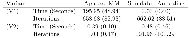
First we compare the running times of the proposed algorithms and the brute force ap-proach. We consider two settings: (p= 100, T = 1000) and (p= 500, T = 500). In the setting (p= 100, T = 1000), 100 independent runs of Algorithms 2 and 3 are performed and the average run-times are reported in Table 1. In the setting (p= 500, T = 500) 10 independent runs of Algorithms 2 and 3 are used, and the results are presented in Table 2. We compare these times to results from one simulation run of the brute-force approach, the results of which are given in the description (caption) of Tables 1 and 2.

We consider two stopping criteria for Algorithm 2 or 3. The first criterion stops the iterations if

1

T|τ

(k)

−τ?|<0.005 and

kθ(₁k)−θˆ1kF

kθˆ1kF

+kθ

(k) 2 −θˆ2kF

kθˆ2kF

<0.05, (V1)

where ˆθ1 and ˆθ2 are obtained by performing 1000 proximal-gradient steps at the true τ

Variant

Approx. MM

Simulated Annealing

(V1)

Time (Seconds)

195.95 (48.94)

3.03 (0.40)

Iterations

658.68 (82.93)

662.62 (88.51)

(V2)

Time (Seconds)

0.39 (0.10)

0.48 (0.46)

Iterations

1.03 (0.17)

101.96 (100.29)

Table 1:

Run-times of Algorithm 2 and 3 for (

p

= 100

, T

= 1000). For comparison the

run-time of the brute force algorithm for this problem is 2374

.

82.

Variant

Approx. MM

Simulated Annealing

(V1)

Time (Seconds)

3554.30 (404.24)

94.64 (5.50)

Iterations

939.70 (11.03)

941.70 (16.23)

(V2)

Time (Seconds)

4.27 (1.10)

10.96 (8.26)

Iterations

1.10 (0.32)

111.20 (90.71)

Table 2:

Run-times of Algorithm 2 and 3 for (

p

= 500

, T

= 500). For comparison the

run-time of the brute force algorithm for this problem is 10854

.

44.

change-point sequence τ(k) _{can converge well before θ}(k)

1 and θ

(k)

2 . To illustrate this, we

also explore the alternative approach of stopping the iterations only based onτ(k)_{, namely}

when

1

T|τ

(k)_−τ

?|<0.005. (V2) Finally, we note that we implement the brute force approach by running 500 proximal-gradient steps for each possible value of τ. Note that 500 iterations is typically smaller than the number of iterations needed to satisfy (V1).

Tables 1 and 2 highlight the benefits of Algorithm 2 and Algorithm 3 as the run-time is several orders of magnitude lower than the brute force approach. Additionally, while Algorithm 3 requires more iterations than Algorithm 2 its run-time is typically smaller. The benefits of Algorithm 3 are particularly clear for large values of pandT (under stopping criterion (V1)). The stopping criteria (V2) highlights the fact that theτ(k)_{sequence in the}

proposed algorithms can converge well before theθ-sequences.

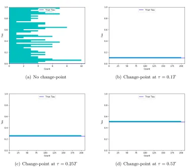
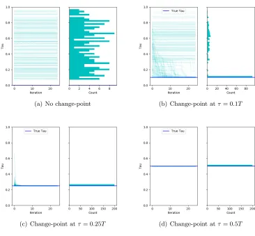
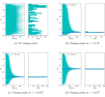
3.2 Behavior of the Algorithm when the Change-Point is at the Edge

We investigate how the brute force algorithm, Algorithm 2, and Algorithm 3 perform when change-points are non-existent or close to the edges. The results for the brute force algorithm are presented in Figure 1, the results for Algorithm 2 are presented on Figure 2 and the results for Algorithm 3 are presented on Figure 3. For Algorithm 2 and Algorithm 3 the figure contains two subfigures, the first showing the sequences {τ(k)_{} of solutions}

(a) No change-point (b) Change-point atτ = 0.1T

(c) Change-point atτ= 0.25T (d) Change-point atτ = 0.5T

(a) No change-point (b) Change-point atτ = 0.1T

(c) Change-point atτ= 0.25T (d) Change-point atτ = 0.5T

(a) No change-point (b) Change-point atτ = 0.1T

(c) Change-point atτ= 0.25T (d) Change-point atτ = 0.5T

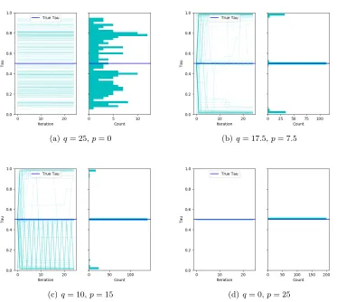
(a)q= 25,p= 0 (b) q= 17.5,p= 7.5

(c)q= 10,p= 15 (d) q= 0,p= 25

Figure 4:

Behavior of the brute force approach for varying signals. Each plot is a histogram

of the final change-point estimate. Based on 200 replications.

3.3 Behavior of the Algorithms when

θ

and

θ

are Similar

Asθ1andθ2get increasingly similar, the location of the change-point becomes increasingly

more difficult to find. We investigate the behavior of the proposed algorithms in such settings. We generate the true precision matricesθ1andθ2 as follows. We draw a random

precision matrix θ with q% non-zero off-diagonal elements, and C1 and C2 two random

precision matrix with p% non-zero off-diagonal elements. We choose C1 and C2 to have

the same diagonal elements. Then we set θ1 = θ+C1 and θ2 =θ+C2, which are then

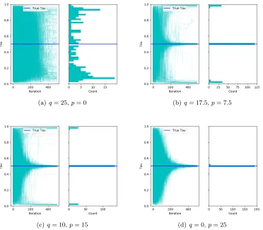
used to generate the data set for the experiment. The ratiop/qis a rough indication of the signal. Figure 4-6 show the behavior of the three algorithms for different values ofq and

(a)q= 25,p= 0 (b) q= 17.5,p= 7.5

(c)q= 10,p= 15 (d) q= 0,p= 25

(a)q= 25,p= 0 (b) q= 17.5,p= 7.5

(c)q= 10,p= 15 (d) q= 0,p= 25

3.4 Sensitivity to the Stopping Criteria in Binary Segmentation

This section considers the stopping condition for the binary segmentation algorithm (see Section 2.2) and how it performs with different configurations. A condition is required for determining when the binary segmentation splitting should reject a change-point and stop running. The stopping condition that we use is the following, stop if

`τ+Cp≥`F,

where `τ is the penalized negative log-likelihood obtained with the additional change-point τ, and `F is the penalized negative log-likelihood without the change-point. The termCis a user-defined parameter.

As mentioned above, the proposed algorithms can diverge when the step-sizeγ is not appropriately selected. In particular the appropriate value ofγis highly dependent on the length of the data set, and the binary segmentation splittings of the data can result in data segments with very different lengths. We use this feature to our advantage. We have chosen not to tuneγto the data segment, and to stop the binary segmentation splitting if the sequence ˆθ₁(k)or ˆθ(₂k) appear to diverge. This has the effect of constraining the lengths of the change-point segments from being too small. We achieve this result without directly setting a minimum length constraint—which be hard to do in practice. We found that stopping the algorithm when||θˆ(_ik)||2

2>2×103 was sufficient for our data.

In the binary segmentation, since the estimates ofθ1andθ2may not have converged by

the end of the search forτ it may be worth continuing the estimation procedure forθ1and

θ2 so that the resulting penalized log-likelihoods are comparable. Hence after each split

from the binary segmentation search, we perform an additional 500 iterations to estimate

θ1 andθ2at the resultingτ.

See Figure 7 for a series of heatmaps showing how often the binary segmentation method finds a given number of change-points for different values of C. These results suggest that the choice ofCin the interval (0,4) is reasonable. These results are produced using Algorithm 3 for speed, however, the results are identical for the other two algorithms considered. Note that since an additional change-point should always improve the log-likelihood, whenC ≤0 we only stop on the secondary stopping condition that ||θˆ_i(k)||2

2>

2×103.

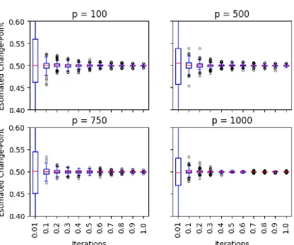
3.5 High Dimensional Experiments

We also investigate the behavior of the proposed algorithms for larger values ofp. We per-formed several (100) runs of Algorithm 3 for T = 1000, and p ∈ {100,500,750,1000}. From these 100 runs we estimate the distributions of the iterates (by boxplots) after 10,100,200, . . . ,1000 iterations. The results are presented in Figure 8. The results show again a very quick convergence towardτ?and this convergence persists even aspgets large.

3.6 A Real Data Analysis

Data from the S&P 500 was collected for the period from 2000-01-01 to 2016-03-03. From this initial sample a subset of stocks (or tickers) was selected for which at least 3000 corresponding observations exist. This produced a sample extending from 2004-02-06 to 2016-03-03, consisting of 3039 observations and 436 stocks. We follow a similar data cleaning procedure to Lafferty et al. (2012), who investigate a comparable problem without change-points. For each stock we generate the log returns, log Xt

Xt−1, and standarize the

resulting returns. Following Lafferty et al. (2012), we then truncate (or clip) all observations beyond three standard deviations of the same mean, thereby limiting unwanted outliers in our sample. The reason for this cleaning procedure is that these outliers often correspond to stock splits instead of meaningful price changes.

For our setting λ = 0.002 andγ = 0.5. We initialize ˆθ(0) _{= (S(τ}(0)_{) +I)}−1 _where

= 10−4 _{and τ}(0) _{is selected randomly. After the simulated annealing run the proximal}

gradient algorithm was run an additional 2000 steps, to produces estimates ofθ1 andθ2.

Here we increase the step-size to γ = 350 to accelerate the convergence. For the binary segmentation we found that selecting the threshold constant,C= 0.005, found a reasonable set of change-points. We found the choice of parameters important in this application, in particular, variation from the values used here can lead the algorithm to diverge. We use the same stopping criterion as with the prior binary-segmentation simulations. That is, a) stop when`τ+Cp≥`F or b) stop when||θˆ

(k)

i ||

2

2>2×103.

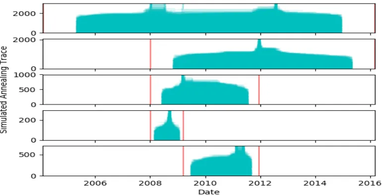
Figure 9 presents the results of the change-point analysis using binary segmentation with Algorithm 4. As a reference we also present the results obtained using binary segmen-tation together with the brute force approach. For the brute force approach, we setγ= 35 and ran 10 iterations for each possible change-point, before running 2000 steps atγ= 350 to get the estimates forθ1 andθ2. The brute force approach took approximately an hour

to run one layer of the search, while simulated annealing took approximately 15 minutes. Figure 9-(a) shows the trace plots from simulated annealing based on 100 replications. The red lines mark the detected time segments. Figure 9-(b) shows the resulting segmentation of the data. We note that simulated annealing and brute force produce slightly differ-ent sets of change-points. This brings up an important point: the resulting solution is a local optimum. Binary segmentation does introduce an element of path dependency to the results so there may be more than one viable set of change-points—in this particular case, the brute force approach starts with the first change-point on August 19th 2011 while simulated annealing starts with January 11th 2008.

(a) Simulated Annealing trace plots from 100 replications. The red lines represent the prior set of relevant change-points.

(b) Simulated annealing (top) and brute force segmentations of the data.

Figure 9:

Change-points analysis of the S&P 500 data set over the period 2004-02-06 to

2016-03-03.

Figure 10:

Adjacency matrices between stocks based on estimated precision matrices ˆ

θ

for each time segment. A black dot represents an edge between two stocks.

AA+. The August 19th 2011 brute force change-point more precisely identifies this August downturn.

Given that the change-point set identified seems sensible, we then investigate what the corresponding ˆθ estimates look like, and whether any interesting conclusions can be drawn from our estimates. Here we focus only on the simulated annealing change-point set. See Figure 10 for a plot of the adjacency matrix for each ˆθ estimate. The black squares correspond to non-zero edges and he yellow boxes correspond to Global Industry Classification Standard (GICS) sectors. These results tell an intuitive story about how the economy behaves during financial crises. Following both the collapse of Lehamn Brother’s and the events of August 2011, we see a dramatic increase in connectivity between returns even outside of GICS sectors. To get a better sense of this see Figure 11 for a similar series of plots where edges are summed over each sector. Figure 12 gives an expanded version of the summed edge plot for the first ˆθ estimate, as well as the corresponding sector labels for reference. Again, we can see that during periods of crisis, the off diagonal elements—corresponding to edges between different sectors—become more significant than during periods of general stability.

Figure 11:

Adjacency matrices between sectors for each time segment.

Based on the

number of edges going from stocks of one sector to another as given by the

estimated precision matrices ˆ

θ

.

and the Financial sector for each ˆθ estimate. We can see that during times of crisis, there is considerable connection between Industrials, Information Technology, Consumer Discretionary, and to a lesser extend Healthcare, and the Financial sector. Consumer Staples, Utilities, and Materials appear to be more stable during these periods and do not experience as much correlation with Financials. This might suggest that our method could be used as a tool to identify investment strategies that are likely to be resilient to periods of crisis in the market.

4. Proofs

4.1 Proof of Theorem 5

We will need the following lemma.

Lemma 12 Set

g(θ)def= −log det(θ) +Tr(θS),

and φ(θ)def= g(θ) +λ

αkθk1+1−α 2 kθk

2

F

, θ∈ M+

p,

for some symmetric matrix S,α∈(0,1), andλ >0. Fix0< b < B≤ ∞.

1. Forθ, ϑ∈ M+

p(b, B), we have

g(θ) +h∇g(θ), ϑ−θi+ 1

2B2kϑ−θk 2

F≤g(ϑ)

≤g(θ) +h∇g(θ), ϑ−θi+ 1

2b2kϑ−θk 2

Figure 12:

Number of edges between the financial sector and the remaining sectors, for

each time segment. Based on the estimated precision matrices ˆ

θ

.

More generally, Ifθ, ϑ∈ M+

p, then

g(ϑ)−g(θ)− h∇g(θ), ϑ−θi ≥ kϑ−θk 2

F

4kθk2 kθk2+1₂kϑ−θkF

.

2. Letγ∈(0, b2], andθ,θ, θ¯ 0∈ M+p(b, B). Suppose that

¯

θ= Proxγλ θ−γ(S−θ−1)

,

then

2γ φ(¯θ)−φ(θ0)+

θ¯−θ0

2

F≤

1− γ

B2

kθ−θ0k2_F.

Proof The first part of (1) is Lemma 12 of Atchad´e et al. (2015), and Part (2) is Lemma 14 of Atchad´e et al. (2015). The second part of (1) can be proved along similar lines. For completeness we give the details below.

Takeθ0, θ1∈ M+p. By Taylor expansion we have

g(θ1)−g(θ0)− h∇g(θ0), θ1−θ0i=−

Z 1

0

(θ0+tH)−1−θ−01, H

dt,

whereH def= θ1−θ0. We have (θ0+tH)−1−θ0−1=−tθ

−1

0 H(θ0+tH)−1, which leads to

g(θ1)−g(θ0)− h∇g(θ0), θ1−θ0i=

Z 1

0

Tr θ−₀1H(θ0+tH)−1H

Ifθ0=P

p

i=1ρjuju0jis the eigendecomposition ofθ0, we see thatTr θ−01H(θ0+tH)−1H

=

Pp

j=1 1

ρju 0

jH(θ0+tH)−1Huj. Hence

g(θ1)−g(θ0)− h∇g(θ0), θ1−θ0i ≥

p

X

j=1

kHujk22

Z 1

0

tdt

kθ0k2(kθ0k2+tkHkF)

≥

Pp

j=1kHujk 2 2

4kθ0k2 kθ0k2+1 2kHkF

,

and the result follows by noting thatPp

j=1kHujk 2

2=kHk2F.

Set

F(τ, θ1, θ2) =g1,τ(θ1) +λ1,τp(θ) +g2,τ(θ2) +λ2,τp(θ2),

F=F(ˆτ,θˆ1,ˆτ,θˆ1,τˆ) the value of Problem (3), andFk=F(τ(k), θ

(k) 1 , θ

(k) 2 )− F.

Lemma 13 Suppose thatγ∈(0,b21∧b 2

2], and forj= 1,2,θ (0)

j ∈ M

+

p(bj,Bj). Thenlimk

θ

(k)

1 −θˆ1,τ(k)

_F=

0,limk

θ

(k)

2 −θˆ2,τ(k)

_F= 0. Furthermore the sequence{Fk} is non-increasing, andlimkFk exists.

Proof We know from Lemma 2 that forγ∈(0,b21∧b 2 2], andθ

(0)

j ∈ M

+

p(bj,Bj), we have

θ(_jk)∈ M+

p(bj,Bj) for allk≥0, for j= 1,2. We have,

Fk+1− Fk =F(τ(k+1), θ

(k+1)

1 , θ

(k+1)

2 )− F(τ

(k)

, θ(₁k+1), θ(₂k+1))

+F(τ(k), θ₁(k+1), θ₂(k+1))− F(τ(k), θ₁(k), θ(₂k)).

By definition, F(τ(k+1), θ₁(k+1), θ(₂k+1))− F(τ(k), θ₁(k+1), θ(₂k+1)) ≤ 0, and by Lemma 12-Part(2),

F(τ(k), θ₁(k+1), θ₂(k+1))− F(τ(k), θ₁(k), θ₂(k))

≤ − 1

2γ

θ

(k+1)

1 −θ

(k) 1 2 F− 1 2γ θ

(k+1)

2 −θ

(k) 2 2 F

It follows that

Fk+1≤ Fk− 1 2γ

θ

(k+1)

1 −θ

(k) 1 2 F− 1 2γ θ

(k+1)

2 −θ

(k) 2 2 F,

which implies that

lim k

θ

(k+1)

1 −θ

(k) 1

_F= 0, and lim_k θ

(k+1)

2 −θ

(k) 2

_F= 0. (15)

It also implies that the sequence {Fk} is non-increasing and bounded from below by 0. Hence converges. Another application of Lemma 12 gives

2γF(τ(k), θ₁(k+1), θ(₂k+1))− F(τ(k),θˆ_1,τ(k),θˆ_2,τ(k))

+ θ

(k+1)

1 −θˆ1,τ(k)

2 F + θ

(k+1)

2 −θˆ2,τ(k)

2 F ≤

1− γ

B2₁

θ

(k)

1 −θˆ1,τ(k)

2 F +

1− γ

B2₂

θ

(k)

2 −θˆ2,τ(k)

And notice thatF(τ(k)_{, θ}(k+1)

1 , θ

(k+1)

2 )− F(τ(k),θˆ1,τ(k),θˆ_2,τ(k))≥0. Hence

θ

(k+1)

1 −θˆ1,τ(k)

2 F + θ

(k+1)

2 −θˆ2,τ(k)

2 F ≤

1− γ

B2₁

θ

(k)

1 −θˆ1,τ(k)

2 F +

1− γ

B2₂

θ

(k)

2 −θˆ2,τ(k)

2 F ,

which can be written as

γ

B2₁

θ

(k)

1 −θˆ1,τ(k)

2 F + γ B2₂

θ

(k)

2 −θˆ2,τ(k)

2 F≤ θ

(k+1)

1 −θ

(k) 1 2 F + θ

(k+1)

2 −θ

(k) 2 2 F

−2Dθ(₁k+1)−θ₁(k), θ₁(k+1)−θˆ_1,τ(k)

E

−2Dθ(₂k+1)−θ₂(k), θ₂(k+1)−θˆ_2,τ(k)

E

.

Since {θ(₁k)}, {θ(₂k)} {θˆ_1,τ(k)}, and{θˆ_2,τ(k)} are bounded sequence, and given (15), letting k→ ∞, we conclude that

lim k

θ

(k)

1 −θˆ1,τ(k)

_F= 0, and lim_k θ

(k)

2 −θˆ2,τ(k)

_F= 0.

Proof of Theorem 5Let >0 as in H1. By Lemma 13, there existk0≥1 such that for

allk≥k0,

θ

(k+1)

1 −θˆ1,τ(k)

_F≤, and θ

(k+1)

2 −θˆ2,τ(k)

_F≤. Since

τ(k+1)=Argmin_t∈T Ht|θ(₁k+1), θ(₂k+1),

using H1 we conclude that for allk≥k0,

τ

(k+1) −τ?

≤κ τ

(k) −τ?

+c≤κ

k−k0+1

τ

(k0)_−τ

?

+

c

1−κ,

which implies the stated result.

4.2 Proof of Theorem 9

We introduce some more notation. Given M ∈ Rp×p the sparsity structure of M is the

matrixδ∈ {0,1}p×p _{such thatδ}

jk=1{|Mjk|>0}. In particular we will writeδ?,j (j = 1,2) to denote the sparsity structure ofθ?,j. Given matrices A∈Rp×p, andδ∈ {0,1}p×p, we

will use the notation Aδ (resp. Aδc) to denote the component-wise product of A and δ (respA and 1−δ). Givenj ∈ {1,2}, we define

Cj

def

= nM ∈ Mp: kMδc

?,jk1≤7kMδ?,jk1.

o

. (16)

We will need the following deviation bound.

Lemma 14 Suppose that Xi ind

∼ N(0, θ−_i1),i= 1, . . . , N, where θi∈ M+p. We set Σi

def

= θ−_i1, and define

and suppose that κ_i(2) > 0 for i = 1, . . . , N. Set GN

def

= N−1PN

i=1(XiXi0 −θ −1

i ). Then for 0< δ≤2minkκk(2)

maxk¯κk(2)

2

, we have

P

kGNk∞>

max k ¯κk(2)

δ

≤4p2e−N δ 2 4 .

Proof The proof is similar to the proof of Lemma 1 of Ravikumar et al. (2010), which itself builds on Bickel and Levina (2008). For 1≤i, j ≤p, arbitrary, setZ_ij(k)=Xk,iXk,j, andσ(_ijk)= Σk,ij, so that the (i, j)-th component ofGN isN−1PN_k=1(Z

(k)

ij −σ

(k)

ij ). Suppose thati6=j. The casei=j is simpler. It is easy to check that

N

X

k=1

h

Z_ij(k)−σ_ij(k)i=1 4

N

X

k=1

h

(Xk,i+Xk,j)2−σ

(k)

ii −σ

(k)

jj −2σ

(k)

ij i −1 4 N X k=1 h

(Xk,i−Xk,j)2−σ

(k)

ii −σ

(k)

jj + 2σ

(k)

ij

i

.

Notice thatXk,i+Xk,j ∼N(0, σ

(k)

ii +σ

(k)

jj +2σ

(k)

ij ), andXk,i−Xk,j∼N(0, σ

(k)

ii +σ

(k)

jj −2σ

(k)

ij ). It follows that for allx≥0,

P " N X k=1 h

Z_ij(k)−σ_ij(k)i

> x # ≤P " N X k=1

a(_ijk)(Wk−1)

>2x

# +_P " N X k=1

b(_ijk)(Wk−1)

>2x

#

,

whereW1:N i.i.d.

∼ χ21,a (k)

ij =σ

(k)

ii +σ

(k)

jj + 2σ

(k)

ij , andb

(k)

ij =σ

(k)

ii +σ

(k)

jj −2σ

(k)

ij . For anyx≥0 and a sequencea= (a1, . . . , aN) of positive numbers, with|a|∞= maxi|ai|,|a|2=

pP

ia

2

i, we write

2x= 2|a|2

_x

2|a|2

+ 2|a|∞

_4|a|2 2

2x|a|∞

x

2|a|2

2

.

Therefore if 2x|a|∞ ≤ 4|a|22, we can apply Lemma 1 of Laurent and Massart (2000) to

conclude that P N X k=1

ak(Wk−1)

≥2x

!

≤2e−

x2 4|a|2

2.

In particular, we can apply the above bound withx=|a|∞N δ forδ∈(0,2 minja

2 i

maxia2i

] to get that P N X k=1

ak(Wk−1)

≥2|a|∞N δ

!

≤2e−N δ 2 4 .

In the particular case above, a(_ijk)=σ(_iik)+σ_jj(k)+ 2σ(_ijk)=u0Σ(k)_{u, whereu}

i=uj= 1, andur= 0 forr /∈ {i, j}. And

minku0Σ(k)u

maxku0Σ(k)u

≥ minkκk(2) maxk¯κ(2).

The following event plays an important role in the analysis. En def = \ τ∈T ₁

λ1,τ

k∇g1,τ(θ?,1)k∞≤

α

2, and 1

λ2,τ

k∇g2,τ(θ?,2)k∞≤

α

2

, (17)

Lemma 15 Under the assumptions of the theorem

P(En)≥1− 8

pT.

Proof We have

P(Enc)≤P

max τ∈T

1

λ1,τ

k∇g1,τ(θ?,1)k∞>

α 2 +P max τ∈T 1

λ2,τ

k∇g2,τ(θ?,2)k∞>

α

2

.

We show how to bound the first term. A similar bound follows for g2,τ by working on the reversed sequence X(T), . . . , X(1). We have ∇g1,τ(θ) = ₂τ_T(S1(τ)−θ−1). Setting

U(t) def= X(t)(X(t))0−E X(t)(X(t))0, we can write

∇g1,τ(θ?,1) =

1 2T

τ

X

t=1

U(t)+(τ−τ?)+ 2T (θ

−1

?,2−θ

−1

?,1),

wherea+ def

= max(a,0). Hence by a standard union-bound argument,

P

max τ∈T

1

λ1,τ

k∇g1,τ(θ?,1)k∞>

α 2 ≤X τ∈T P τ X t=1

U(t)

∞

> αλ1,τT−(τ−τ?)+kθ?,−12−θ

−1

?,1k∞

!

.

Given the choice ofλ1,τ in (8), αλ1,τT /2 = 2

√

3¯κpτlog(pT)≥(τ−τ?)+kθ−?,12−θ

−1

?,1k∞,

by assumption (11). In view of (10) we can apply Lemma 14 to deduce that

P

max τ∈T

1

λ1,τ

k∇g1,τ(θ?,1)k∞>

α 2 ≤ X τ∈T P 1 τ τ X t=1

U(t)

_∞

> αλ1,τT

2τ

!

≤ 4T p2e−τ4 αλ1,τ T

2τκ¯ 2

≤ 4 exp (2 log(pT)−3 log(pT))≤ 4

pT.

Lemma 16 Under the assumptions of the theorem, and on the eventEn, we have

ˆ

θ1,τ−θ?,1

_F≤Aκ¯kθ?,1k

2 2

r

s1log(pT)

τ , and ˆ

θ2,τ−θ?,2

_F≤Aκ¯kθ?,2k

2 2

r

s2log(pT)

T−τ ,

Proof Fix j ∈ {1,2}, and τ ∈ T. Set ¯gj,τ(θ)

def

= gj,τ(θ) + (1−α)λj,τkθkF/2, and recall

thatφj,τ(θ)

def

= gj,τ(θ) +λj,τ℘(θ). Henceφj,τ(θ) = ¯gj,τ(θ) +αλj,τkθk1. By a very standard argument that can be found for instance in Negahban et al. (2012), it is known that on the eventEn, and ifαsatisfies (9) then we have ˆθj,τ−θ?,j∈ Cj, where the conesCj are as defined in (16). We write

φj,τ(ˆθj,τ)−φj,τ(θ?,j) =

D

∇gj,τ(θ?,j) + (1−α)λj,τθ?,j,θˆj,τ−θ?,j

E

+¯gj,τ(ˆθj,τ)−g¯j,τ(θ?,j)−

D

∇¯gj,τ(θ?,j),θˆj,τ−θ?,j

E

+αλj,τ

kθˆj,τk1− kθ?,jk1

.

OnEn, ˆθj,τ−θ?,j∈ Cj. Therefore

αλj,τ

k

ˆ

θj,τk1− kθ?,jk1

≤αλj,τ

ˆ

θj,τ−θ?,j

₁≤8αλj,τ

√ sj ˆ

θj,τ−θ?,j

_F, and D

∇gj,τ(θ?,j) + (1−α)λj,τθ?,j,θˆj,τ−θ?,j

E

≤λj,τ

2 (α+ 2(1−α)kθ?,jk∞)

ˆ

θj,τ −θ?,j

₁

≤4λj,τ(α+ 2(1−α)kθ?,jk∞)

√ sj ˆ

θj,τ−θ?,j

_F.

Supposej = 1. The case j = 2 is similar. We then set ∆1,τ

def

= ˆθ1,τ −θ?,1, and use the

second part of Lemma 12 (1) to deduce that

¯

g1,τ(ˆθ1,τ)−¯g1,τ(θ?,1)−

D

∇¯g1,τ(θ?,1),θˆ1,τ−θ?,1

E

≥g1,τ(ˆθ1,τ)−g1,τ(θ?,1)−

D

∇g1,τ(θ?,1),θˆ1,τ−θ?,1

E

≥ τ

2T

k∆1,τk2F

2kθ?,1k2(2kθ?,1k2+k∆1,τkF) .

Setc1= _4Tkθτ

?,1k22

,c2= 4λ1,τ

√

s1(3α+ 2(1−α)kθ?,1k∞). Sinceφ1,τ(ˆθ1,τ)−φ1,τ(θ?,1)≤0,

the above derivation shows that on the eventEn,

c1k∆1,τk

2

F

2 +_kθ1

?,1k2k∆1,τkF

−c2k∆1,τkF≤0,

Under the assumption thatc1≥2c2/kθ?,1k2 (which we impose in (10)), this implies that

k∆1,τk_F≤ 4c2

c1

≤Aκ¯kθ?,1k22

r

s1log(pT)

τ ,

whereA= 16×20×√48, as claimed.

Proof of Theorem 9Forτ∈ T, let

r1,τ

def

= A¯κkθ?,1k22

r

s1log(pT)

τ , r2,τ

def

= Aκ¯kθ?,2k22

r

s2log(pT)