Quantification Under Prior Probability Shift: the Ratio
Estimator and its Extensions
Afonso Fernandes Vaz [email protected]
Rafael Izbicki [email protected]
Rafael Bassi Stern [email protected]
Department of Statistics
Federal University of S˜ao Carlos S˜ao Carlos, SP 13565-905, Brazil
Editor:Charles Elkan
Abstract
The quantification problem consists of determining the prevalence of a given label in a tar-get population. However, one often has access to the labels in a sample from the training population but not in the target population. A common assumption in this situation is that of prior probability shift, that is, once the labels are known, the distribution of the features is the same in the training and target populations. In this paper, we derive a new lower bound for the risk of the quantification problem under the prior shift assump-tion. Complementing this lower bound, we present a new approximately minimax class of estimators, ratio estimators, which generalize several previous proposals in the literature. Using a weaker version of the prior shift assumption, which can be tested, we show that ratio estimators can be used to build confidence intervals for the quantification problem. We also extend the ratio estimator so that it can: (i) incorporate labels from the target population, when they are available and (ii) estimate how the prevalence of positive labels varies according to a function of certain covariates.
Keywords: quantification, prior probability shift, data set shift, domain shift, semi-supervised learning
1. Introduction
In several applications of binary classifiers, predicting the labels of individual observations per se is less important than evaluating the proportion of each label on an unlabeled target data set. The latter task is called quantification (Forman, 2008). For example, a company may be interested in evaluating the proportion of users who like each of their products, without access to labeled reviews of these products.
A common approach to such a problem is to (i) train a classifier for the user’s evaluation based on labeled reviews of other products, and (ii) apply this classifier to the unlabeled target set and use the proportion of users who are classified as liking the product as an estimator. However, it is known that this two-step approach, known as “classify and count”, fails because of domain shift (Forman, 2006; Tasche, 2016). In order to deal with this problem, several improvements have been proposed under an assumption named prior shift (Saerens et al., 2002; Forman, 2008; Bella et al., 2010; Barranquero et al., 2015). A particular estimator that successfully performs quantification is the adjusted count (AC) estimator
c
(Gart and Buck, 1966; Saerens et al., 2002; Forman, 2008). Part of the success of the AC estimator is explained in Tasche (2017) by showing that it is Fisher consistent. However, there are more properties one might desire of an estimator.
In order to investigate these properties, Vaz et al. (2017) introduces the ratio estimator, which is a generalization of the AC estimator. Vaz et al. (2017) derives the asymptotic mean squared error of the ratio estimator. Here, we show that the ratio estimator is approximately minimax and consistent under the prior probability shift assumption. In order to derive this result, we prove a new lower bound for the risk of the quantification problem under the prior shift assumption. This lower bound is general and applies to every method under the prior probability shift assumption. We also derive a central limit theorem for the ratio estimator which helps to explain its good performance and leads to a method for building confidence intervals for the quantification problem. This result also allows us to propose a new type of ratio estimator based on Reproducing Kernel Hilbert spaces. Since the AC estimator and the method in Bella et al. (2010) are special cases of the ratio estimator, they benefit from all of the results above.
It is important to evaluate whether the prior probability shift assumption indeed holds, otherwise the AC method can perform poorly (Tasche, 2017). We show that the ratio estimator works under an assumption that is less stringent than the prior shift assumption. Moreover, we show how this assumption can be tested. We are not aware of other methods to test the prior shift and related assumptions.
We also generalize the ratio estimator to two extensions of the quantification problem. In the first scenario, some labels are available in the target population. The combined estimator extends the ratio estimator in order to incorporate these labels and obtain a larger effective sample size. The second scenario considers that the prevalence of each label varies according to additional covariates. This generalization allows one to use unlabeled data to identify e.g. how the approval of a product varies with age. In this scenario, we introduce the regression ratio estimator, which offers improvements over the standard methods that are used in sentiment analyses (Wang et al., 2012).
Section 2 discusses the standard quantification problem under the prior probability shift assumption. Subsection 2.1 provides new lower bounds for the risk in this scenario. Subsection 2.2 introduces the ratio estimator, uses the result from the previous subsection to show that it is approximately minimax and also derives its convergence rate and a central limit theorem. Subsection 2.3 uses the asymptotic behavior of the ratio estimator to propose a new type of ratio estimator based on Reproducing Kernel Hilbert spaces. Finally, the ratio estimator requires a weaker version of prior probability shift to obtain consistency. Subsection 2.4 discusses a new algorithm for testing this assumption.
Section 3 proposes extensions of the ratio estimator to scenarios which are more general than the standard quantification problem. Subsection 3.1 proposes the combined estimator, for cases in which some labels are available in the population of interest. Subsection 3.2 proposes the ratio regression estimator, for the situation in which the prevalence of a given label varies according to a covariate. All proofs are presented in the appendix; code and
data used for the experiments is available at https://github.com/afonsofvaz/ratio_
2. Quantification under prior probability shift
In order to formally approach the quantification problem, we use the same notation as
in Wasserman (2006). If Z1 ∈ Rd1 and Z2 ∈ Rd2 are random vectors and R ⊂ Rd1, then
P(Z1 ∈R|Z2) is the conditional probability thatZ1is inRgivenZ2. UsingP, one can obtain
FZ1|Z2,fZ1|Z2,E[Z1|Z2], andV[Z1|Z2] which are, respectively, the conditional distribution,
density, expected value and variance ofZ1givenZ2. Marginal properties ofZ1are indicated
by omitting the conditioning random variable. Also, if (Zn)n∈N is a sequence of random
vectors, then Zn
a.s.
→ Z, Zn
P
→ Z, and Zn Z indicate respectively, that Zn converges
almost surely, in probability, and in distribution toZ. In order to express the rate at which
convergence occurs, it is useful to use O and Ω notation. If (an)n∈N is a sequence in R,
thenan=O(g(n)) if there existscsuch that, for everyn,an≤c·g(n) andan= Ω(g(n)) if
there exists csuch that, for every n,an≥c·g(n). Finally,I is the indicator function. An
expression such as I(g(X)∈A) is equal to 1 when g(X)∈A and to 0 wheng(X)∈/ A.
In the quantification problem, for each sample instance i∈ {1, . . . , n}, (Xi, Yi, Si) is a
vector of random variables such that Xi ∈Rd are features,Yi ∈ {0,1} is a label of interest
and Si ∈ {0,1} is the indicator that this instance has been labeled. That is, whenever
Si = 0, thenYi is not observed. Note that Si can be random.
In the above framework, some subsets of the instances are frequently used. The sets
Ak := {i ∈ {1, . . . , n} : Si = k} represent the labeled (k = 1) and unlabeled (k = 0)
instances. Similarly, Ak,j := {i∈ {1, . . . , n} :Si = k andYi = j} represent the instances
that are labeled (k= 1) or unlabeled (k= 0) and have a positive (j= 1) or a zero (j= 0)
label. Also the number of instances that are unlabeled, labeled or that have label j are
denoted, respectively, by nU :=|A0|,nL:=|A1|and nj :=|A1,j|.
In a quantification problem, one wishes to estimate θ := P(Y = 1|S = 0), that is, the
prevalence of positive labels among unlabeled samples. This prevalence is not assumed to
be the same as the one over labeled sets,P(Y = 1|S = 1). The estimator forθ can depend
only on the available data, that is, the features of all instances and the labels that were obtained. Formally, letting Zij denote (Zi, . . . , Zj), a valid estimator is a function of Xn1, S1n and (Yi)i∈A1. The set of all such valid estimators is denoted byS.
In the standard formulation of the prior probability shift problem, {(Xi, Yi)}i∈A0 is
called the target population (since the labels are unavailable), and {(Xi, Yi)}i∈A1 is called
the training population (Tasche, 2017). It is common for both populations to be i.i.d.,
Assumption 1
• (S1,X1, Y1), . . . ,(Sn,Xn, Yn) are independent.
• For every s∈ {0,1}, (X1, Y1)|S1=s, . . . ,(Xn, Yn)|Sn=s are identically distributed.
Unless additional assumptions are made, it is not possible to learn aboutθ using solely
the observed data. One assumption that allows learning about θ is the prior probability
shift, which states that “the class-conditional feature distributions of the training and test sets are the same” (Fawcett and Flach, 2005). Prior shift is formalized in Assumption 2.
Although Assumption 2 is written in a different way than in papers such as
Moreno-Torres et al. (2012), the content is similar. While Moreno-Torres et al. (2012) uses a
subscript on the probability function to determine which is the reference population, we
perform this task using the random variable, S. For instance, the probability that an
instance from the target population has the label “1” is referred in previous notation and
in this paper, respectively, as Ptg(Yi = 1) and P(Yi = 1|Si = 0). Using this translation,
Assumption 2 is the same as the prior probability shift in Moreno-Torres et al. (2012). Assumption 2 holds if and only if fX|Y,S=0 ≡fX|Y,S=1, that is,Ptg(x|y)≡Ptr(x|y).
2.1. Lower bound on the risk for quantification under prior probability shift
Under Assumptions 1 and 2 it is possible to learn aboutθfrom the features and labels that
are available in the quantification problem. For example, one can use the features and labels
in the training population to learn about fX|Y=0 and fX|Y=1. Also, if these densities are
sufficiently different, then one can combine the information about them to the features in the target population to learn about the unknown labels in this population and, therefore,
about θ. Definition 1 formally presents two classes in which the possible values of fX|Y=0
and fX|Y=1 are separable.
Definition 1 Let fi(x) =fX|Y=i(x), , K >0 and g:Rd→R be a non-constant function.
(
FL1,:={(f0, f1) :kf0−f1k1 ≥} Fg,K,:=
(f0, f1) :Efi[g(X)
2|Y =i]≤K, and |E
f1[g(X)|Y = 1]−Ef0[g(X)|Y = 0]| ≥
Under the classes in Definition 1 it is possible to learn about θ and the learning rate
depends on both the number of labeled and unlabeled instances. A lower bound for how
these sample sizes affect the rate at which one learns aboutθ is presented in Theorem 3.
Definition 2 Let F be a collection of(f0, f1). The minimax rate, M(F), for estimating θ
under the squared loss, F, and Assumptions 1 and 2 is
M(F) = inf
b θ∈S
sup
(f0,f1)∈F;θ∈[0,1]
Ef0,f1,θ
(θb−θ)2
S1n
Theorem 3 M(FL1,)≥Ω(max(n
−1
L , n
−1
U ))and M(Fg,K,)≥Ω(max(n−L1, n
−1
U )).
Theorem 3 shows that it is not possible to obtain an estimator for θ which has
con-vergence rate faster than Ω(max(n−L1, n−U1)). In particular, it is not possible to learn θ by
observing solely a limited amount of labels. The following subsection introduces the ratio
estimator for θ, which achieves the lower bound in Theorem 3 under Fg,K,.
2.2. The ratio estimator and its theoretical properties
Definition 4 (Ratio estimator) Let g:Rd−→ R. The untrimmed ratio estimator for θ
based on g, θbU R, is
b θU R :=
P
i∈A0g(Xi)
nU −
P
i∈A1,0g(Xi)
n0
P
i∈A1,1g(Xi)
n1 −
P
i∈A1,0g(Xi)
Sinceθ∈[0,1], the ratio estimator, θbR, is
b
θR= max(0,min(1,θbR))
The ratio estimator generalizes estimators which were previously proposed in the litera-ture. This fact follows from observing that the terms in the untrimmed ratio estimator are
sample averages of g(X) among three groups of instances: unlabeled instances, instances
labeled as 0, and instances labeled as 1. For instance, the adjusted count (AC) estimator (Gart and Buck, 1966; Saerens et al., 2002; Forman, 2008; Tasche, 2017) is the a ratio
estimator when g(x) ∈ {0,1}, that is, g(x) is the output of a classifier for Y. Also, the
estimator in Bella et al. (2010) is a ratio estimator when g(x) =Pb(Y = 1|x), that is, g(x)
is a soft classifier forY.
Remark 5 The ratio estimator can be generalized to the case in which Yi ∈ {0,1, . . . , k}. In this case, letg:Rd→Rk be a fixed function. By definingGas a k×(k+ 1) matrix such that Gi,j =E[gi(X)|Y = j−1, S = 1], p ∈Rk+1 such that pi = P(Y = j−1|S = 0), and
g∈Rk such that gi=E[gi(X)|S= 0], θbU R is obtained by solving the linear system
( b
g =Gb·θbU R
1 =1t·θbU R
, where bgi = P
k∈A0gi(Xk) nU
and Gbi,j = P
k∈A1,jgi(Xk)
nj
Since θbU R might have negative components, it is generally inadmissible according to the
squared error (de Finetti, 2017)[p.90-91] that is, there exist estimators which have a squared error strictly smaller than θbU R. The ratio estimator, θbR satisfies this property and is the
projection of θbU R onto the simplex (Michelot, 1986): θbR= arg minpˆ: ˆp≥0,P
ipˆi=1kbθU R−pˆk
2 2.
Similarly to the AC estimator (Tasche, 2017), the ratio estimator is Fisher consistent
under weak assumptions.1. They are described in Assumptions 3 and 4.
Assumption 3 (Weak prior shift) The function,g, is such that g(X)n1 is stochastically independent of Sn1 conditionally onY1n=y1n.
Assumption 4 (Separability) The function, g, is such that
1. E[g(Xi)|Yi =j, Si= 1] are defined, for j∈ {0,1}.
2. E[g(Xi)|Yi = 1, Si = 1]−E[g(Xi)|Yi = 0, Si = 1]6= 0
The condition in Assumption 3 is a relaxed type of prior probability shift that is strictly
weaker than Assumption 2. Assumption 4 requires two more conditions ofg(x). According
to condition 1, the population versions of the expectations in Definition 4 are defined. Condition 2 states that the ratio estimator calculated on these population parameters is defined, that is, there is no division by 0.
Theorem 6 Under Assumptions 1, 3 and 4, θbU R and θbR are Fisher consistent for θ.
It is also possible to guarantee a finite population bound on the mean squared error of
b
θR. This result is obtained in Theorem 7, which substitutes Assumption 4 by the stronger
condition that (f0, f1)∈ Fg,K,.
Theorem 7 Under Assumptions 1 and 3,
sup
(f0,f1)∈Fg,K,
Ef0,f1
b θR−θ
2
S1n
≤ O(max(n−L1, n−U1))
Under the assumptions of Theorem 7, if nU nL, then the convergence of the mean
squared error of the ratio estimator is the same as the one that would have been obtained
if one observed solely nL labels from the target population and used the sample’s label
proportions to estimate θ. The same type of result cannot generally be obtained for the
untrimmed ratio estimator, since the trimming is necessary to guarantee that the ratio of random variables does not have infinite variance. While these conclusions are similar to the ones obtained from Theorem 3 in Lipton et al. (2018), there exist two main differences. First, while the former assumes that there are 2 labels only, the latter applies to an arbitrary
number of labels. Second, Theorem 7 upper bounds the squared error byO(max(n−L1, n−U1)),
which is slightly tighter than the bound ofOmax
lognL
nL ,
lognU nU
in Lipton et al. (2018). It follows from Theorem 3 and Theorem 7 that the ratio estimator satisfies several desirable properties. These properties are presented in Definition 8 and Corollary 9.
Definition 8 Let S andF be, respectively, the classes of estimators and distributions over the data under consideration. An estimatorθb∗ ∈ S is approximately minimax for estimating θ under the squared error loss if
O sup
(f0,f1)∈Fg,K,
Ef0,f1
b θ∗−θ2
S1n !
= Ω inf
b θ∈S
sup
(f0,f1)∈F;θ∈[0,1]
Ef0,f1,θ
(θb−θ)2
S1n !
That is, the squared error of θb∗ attains the optimal rate of convergence.
Corollary 9 Under Assumptions 1 and 3, if there exists , K > 0 such that (f0, f1) ∈ Fg,K,, then θbR is consistent for θ in probability and in L2 asnU
P
→ ∞ and nL→ ∞P . Also, under Assumptions 1, 3, and Fg,K,,θbR is approximately minimax.
Corollary 9 shows that the ratio estimator converges to θunder a weaker version of the
prior probability shift assumption and that the rate of this convergence is minimax (i.e., it is the same rate as that of the minimax estimator). Since the estimators from Gart and Buck (1966); Saerens et al. (2002); Forman (2008); Bella et al. (2010) are particular cases
of the untrimmed ratio estimator, their trimmed versions also converge toθunder the weak
prior shift.
The ratio estimator also satisfies a central limit theorem. In order to obtain this result, besides requiring Assumptions 1, 3 and 4, it is also necessary to require that conditionally
on Y,g(X) has bounded variance and that the number of labeled samples goes to infinity.
Assumption 5
1. V[g(Xi)|Yi =j]<∞, for every j∈ {0,1}.
2. There exists h(n)≥0 such thatlimn→∞h(nn) <1, limn→∞h(n) =∞, and hn(Ln) →P 1.
Theorem 10 Define µj := E[g(X1)|Y1 = j], σ2j := V[g(X1)|Y1 = j], pL := limn→∞h(nn), and pj|L:=P(Y =j|S = 1). Under Assumptions 1, 3, 4 and 5,
1. If pL6= 0, then
√
n(bθR−θ) N
0,
(1−θ)σ2
0+θσ12+(µ1−µ0)2θ(1−θ)
1−pL +
(1−θ)2σ2 0
pLp0|L + θ2σ2
1
pLp1|L (µ1−µ0)2
2. If pL= 0, then
p
h(n)(θbR−θ) N
0,
(1−θ)2σ2 0
p0|L + θ2σ2
1
p1|L (µ1−µ0)2
It is possible to use Theorem 10 to obtain an approximate confidence interval forθ. This
interval is obtained by inverting the convergence results in Theorem 10, and substitutingθ
forθbRand the population parameters,µ0,µ1,σ02,σ12,pL,p0|L and p1|L, by their respective
empirical averages. This confidence interval may also be used to test hypothesis such as
H0:θ∈Θ0.
Theorem 10 also provides an approximation for the mean squared error of θbR. This
approximation for the common case in whichnU nLis presented in the following corollary.
Corollary 11 Under Assumptions 1, 3, 4 and 5, if pL= 0 (nU nL), then
MSE(bθR)≈
1
nL(µ1−µ0)2
σ02(1−θ)2
p0|L
+σ
2 1θ2 p1|L
(1)
Corollary 11 brings some insights on how g should be chosen in order for θbR to be an
accurate estimator ofθ. For instance, it shows that one should choosegsuch that |µ1−µ0|
is large and bothσ20 andσ21 are small. This implies that the distributions ofg(X)|Y = 1 and
g(X)|Y = 0 should place most of their masses in regions that are far apart. This conclusion
explains the success of the methods in Forman (2008), in which g(x) is a classifier, and
Bella et al. (2010), in which g(x) is an estimate of P(Y = 1|x).
One of the main deficiencies of the standard AC estimator is that its denominator can be very close to zero, which makes it very unstable (due to a large variance). In order to handle this, we can explicitly use the approximation of the MSE (Corollary 11) to choose
2.3. Choosing g via approximate MSE minimization
One possible criterion for the choice of g is the minimization of M SE(θbR), defined in
Corollary 11. However, the latter depends on unobservable quantities. An alternative is to
minimize an estimate of M SE(θbR). This estimate is presented in Definition 12.
Definition 12 Let θˆbe an estimator of θ and, for each i∈ {0,1}, let
b
µi =n−i 1
X
A1,i
g(Xi) σb 2
i =n
−1
i
X
A1,i
(g(Xi)−µbi) 2
b pi|L=
ni
n0+n1
The empirical MSE of the ratio estimator induced byg, M SE\(g), is
[
MSE(g)≈ 1
nL(µb1−µb0) 2
b
σ02(1−θb)2 b p0|L
+bσ 2 1θb2 b p1|L
!
In order to avoid overfitting, we perform the minimization ofM SE\(g) on a Reproducing
Kernel Hilbert Space (RKHS; Wahba (1990)). More precisely, if K is a Mercer kernel and
HK is the RKHS associated toK, then we chooseg∗ as
g∗ := arg min
g∈HK
[
MSE(g) (2)
In the following, Theorem 13 presents a characterization of g∗ in eq. 2.
Theorem 13 Let K be a Mercer kernel and HK the corresponding RKHS. Also,
• K: the Gram matrix defined for (i, j)∈A21 and such that(K)i,j =K(xi,xj).
• mi: A vector of size |A1| and such that, for eachk∈A1, mi,k = P
j∈A1,iK(xj,xk)
ni .
• M = (m1−m0)(m1−m0)t.
• Σbi: a|A1|×|A1|matrix such that(Σbi)k,lis the sample covariance between(K(xj,xk))j∈A1,i
and (K(xj,xl))j∈A1,i.
• N: a |A1| × |A1|matrix such that N = bθ2 b
p1|LΣb1+
(1−θb)2 b p0|L Σb0.
• w∗= arg minw∈RnL w
tNw
wtMw
The function g∗ in eq. 2 satisfies g∗(x) =P
i∈A1w
∗
iK(x,xi).
The vector, w∗ in Theorem 13 is the eigenvector associated to the largest eigenvalue
in absolute value, λ∗, of the generalized eigenvalue problem, Mw∗ = λ∗Nw∗. If N is
invertible, w∗ is the eigenvector associated to the largest eigenvalue in absolute value of
N−1M. Alternatively, ifN is not invertible one can substitute N in Theorem 12 by (N+
γ1)−1, where1is the identity matrix andγ is a small number that makesN+γ1invertible.
Addingγ to the diagonal also also adds regularization and can therefore lead to an improved
solution. In practice we choose γ via data-splitting.
2.4. Testing the weak prior shift assumption
The following proposition is useful for testing the weak prior shift assumption:
Proposition 14 Under Assumption 3, there exists 0≤p≤1 such that
pFg(X)|S=1,Y=1+ (1−p)Fg(X)|S=1,Y=0=Fg(X)|S=0.
It follows from Proposition 14 that Assumption 3 entails the hypothesis:
H0 :∃0≤p≤1 such thatpFg(X)|S=1,Y=1+ (1−p)Fg(X)|S=1,Y=0=Fg(X)|S=0
In the following, we show how to construct an hypothesis test for H0 when g(x) is
continuous. Since the weak prior shift entails H0, if this test is used to test the weak prior
shift, it will have the correct type I error. However, H0 may hold when Assumption 3 is
false. A specific example in whichH0 is satisfied but Assumption 3 is not satisfied is given
in the following example.
Example 1 If Fg(X)|S=0,Y=1 = Fg(X)|S=0,Y=0 and Fg(X)|S=0,Y=1 = Fg(X)|S=1,Y=1, then
there existsp such thatpFg(X)|S=1,Y=1+ (1−p)Fg(X)|S=1,Y=0=Fg(X)|S=0 (namely, p= 1)
even ifFg(X)|S=1,Y=0 6=Fg(X)|S=0,Y=0. In this case, Assumption 3 does not hold and H0 is
satisfied.
The following statistic, T, measures disagreement withH0:
T = inf
0≤p≤1d
pFbg(X)|S=1,Y=1+ (1−p)Fbg(X)|S=1,Y=0,Fbg(X)|S=0
,
where dis a distance between cumulative distributions, such as the Kolmogorov distance,
and Fb are the empirical cumulative distributions (Wasserman, 2013):
b
Fg(X)|S=1,Y=i(w) =
1
|A1,i|
X
i∈A1,i
I(g(Xi)≤w), Fbg(X)|S=0(w) =
1
|A0|
X
i∈A0
I(g(Xi)≤w).
Algorithm 1, which is presented below, obtains a p-value forH0 based onT. The algorithm
uses kernel smoothers (Wasserman, 2013) to estimate the conditional densities ofg(X) given
Y,f(g(x)|Y = 0) andf(g(x)|Y = 1), by fb(g(x)|Y = 0) andfb(g(x)|Y = 1).
Note that our test is different from those proposed by Saerens et al. (2002) and Lipton et al. (2018). While our test evaluates whether the prior shift assumption is reasonable for
the observed data, the above tests assume prior shift and evaluate whether the prevalence
of positive labels in the unlabeled sample is the same as that in the labeled sample, that is,
P(Y = 1|S= 0) =P(Y = 1|S = 1).
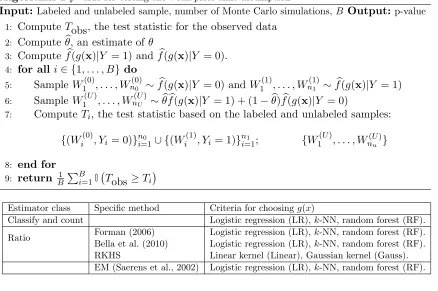
Algorithm 1 p-value for testing the weak prior shift assumption
Input:Labeled and unlabeled sample, number of Monte Carlo simulations, B Output: p-value
1: Compute Tobs, the test statistic for the observed data
2: Compute θb, an estimate of θ
3: Compute fb(g(x)|Y = 1) andfb(g(x)|Y = 0).
4: for alli∈ {1, . . . , B}do
5: Sample W1(0), . . . , Wn(0)0 ∼fb(g(x)|Y = 0) andW (1)
1 , . . . , W (1)
n1 ∼fb(g(x)|Y = 1)
6: Sample W1(U), . . . , Wn(UU)∼θbfb(g(x)|Y = 1) + (1−θb)fb(g(x)|Y = 0)
7: Compute Ti, the test statistic based on the labeled and unlabeled samples:
{(Wi(0), Yi= 0)}ni=10 ∪ {(W (1)
i , Yi= 1)}ni=11 ; {W (U)
1 , . . . , W (U)
nu }
8: end for
9: return B1 PB
i=1I Tobs≥Ti
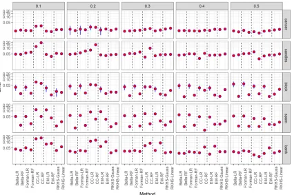
Estimator class Specific method Criteria for choosingg(x)
Classify and count Logistic regression (LR),k-NN, random forest (RF).
Ratio Forman (2006) Logistic regression (LR),k-NN, random forest (RF). Bella et al. (2010) Logistic regression (LR),k-NN, random forest (RF). RKHS Linear kernel (Linear), Gaussian kernel (Gauss). EM (Saerens et al., 2002) Logistic regression (LR),k-NN, random forest (RF).
Table 1: Methods compared in the experiments.
2.5. Experiments
Next, we compare the errors of the ratio estimator and of the classify and count estimator
based on the estimator g when using various methods for obtaining g. We also include
comparisons with the EM methods by Saerens et al. (2002). Table 1 summarizes all the variants that were tested.
We compare the above methods in five data sets: Candles (Freeman et al., 2013; Izbicki and Stern, 2013), Bank Marketing (Moro et al., 2011), SPAM e-mail (Blake, 1998), Wis-consin Breast Cancer (Mangasarian, 1990) and Blocks Classification (Malerba et al., 1996).
Each database was transformed into a prior shift problem by choosing at random n1 (n0)
instances among the ones labeled as 1 (0) to be marked as labeled instances and by choosing
nU instances to be marked as unlabeled. Each unlabeled unit is taken with probability θ
randomly among the instances labeled as 1 in the original data set and with probability
1−θ among those labeled as 0. The quantification sample sizes used in each of these data
sets are described in Table 2. For all data sets we let θ vary in {0.1; 0.2; 0.3; 0.4; 0.5} and repeated the generation and testing 100 times for each of the 11 methods in Table 1.
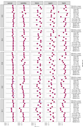
Figure 1 represents the average of the mean squared error (MSE; red point) and a
confidence interval for the MSE (vertical blue bar) for each setting and method2. Figure
2 shows the number of experiments in which each method had the best average MSE,
data set nU nL n1 n0
1 cancer 100 300 150 150
2 candles 300 300 150 150
3 block 800 300 150 150
4 spam 2000 300 150 150
5 bank 10000 300 150 150
Table 2: Sample sizes for each data set.
Figure 1: Root mean square deviation of each method by setting in logarithmic scale.
considering all data sets andθvalues. These plots indicate that the ratio estimator generally
performs better than the classify and count estimator for all choices ofg. The main exception
to this rule occurs whenθ≈0.5 and hence there is no prior shift. Also, the method in Bella
et al. (2010) performs better than the one in Forman (2006) in essentially all scenarios. This suggests that soft classifiers might lead to better ratio estimators than hard classifiers.
Moreover, the best performance is usually achieve whengis based on Random Forest, which
corroborates that choosing a good classifier is key to having a good estimate of θ. The EM
0
1
2
3
4
5
Bella−RF CC−RF EM−RF
RKHS−Gauss
CC−LR
Bella−knn Bella−LR CC−knn EM−LR EM−knn
F
or
man−knn
F
or
man−LR
F
or
man−RF
RKHS−Linear
Method
Frequency
Figure 2: Number of times in which each method presented best MSE.
Figure 3: Mean squared error of the ratio estimator for the multiclass problem.
For all of ratio estimators, data sets and values for θ above, we construct confidence
intervals for θ based on Theorem 10. We find that in all but one scenario the empirical
coverage was at least as high as the specified value of 95%. The empirical coverage in the exception was 94%. The intervals constructed using Theorem 10 seem to be conservative.
Next, we simulate data using the following multiclass setting: X|Y =y∼N(µy,Σ) with
Gaussian
g(x)|S= 1, Y = 0∼N(0,1), g(x)|S= 1, Y = 1∼N(2,1), g(x)|S= 0, Y = 0∼N(γ,1)
g(x)|S= 0, Y = 1∼N(2,1),
P(Y = 1|S= 0) = 0.6,
P(Y = 1|S= 1) = 0.2
Exponential
g(x)|S= 1, Y = 0∼Exp(1), g(x)|S= 1, Y = 1∼Exp(5), g(x)|S= 0, Y = 0∼Exp(γ)
g(x)|S= 0, Y = 1∼Exp(5),
P(Y = 1|S = 0) = 0.6,
P(Y = 1|S = 1) = 0.2
Gaussian-Exponential g(x)|S= 1, Y = 0∼N(1,1), g(x)|S= 1, Y = 1∼Exp(1), g(x)|S= 0, Y = 0∼N(γ,1)
g(x)|S= 0, Y = 1∼Exp(1),
P(Y = 1|S= 0) = 0.6,
P(Y = 1|S= 1) = 0.2
Beta
g(x)|S= 1, Y = 0∼Beta(1,1), g(x)|S= 1, Y = 1∼Beta(1,10), g(x)|S= 0, Y = 0∼Beta(γ,1)
g(x)|S= 0, Y = 1∼Beta(1,10),
P(Y = 1|S = 0) = 0.6,
P(Y = 1|S = 1) = 0.2
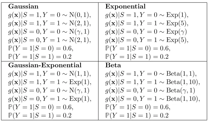
Table 3: Scenarios used for testing the weak prior shift assumption.
P(Y = 2|S = 1) = 0.3 P(Y = 1|S = 0) = 0.25, and P(Y = 2|S = 0) = 0.10. We use
a multivariate logistic regression to compute g1(x) = Pb(Y = 1|x, S = 1) and g2(x) =
b
P(Y = 2|x, S = 1). Figure 3 indicates that the mean squared error of the multiclass ratio
estimator goes to zero as the sample size increases. Moreover, it shows that projecting the raw estimator to the simplex improves the convergence, especially for small sample sizes.
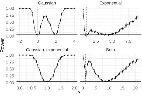
We also evaluate the power of the weak prior shift test in Section 2.4. In order to test the weak prior shift, we generate data according to 4 scenarios, which are presented in table 2.5. In all of these scenarios, the weak prior shift assumption holds for a single value of
γ. Figure 4 presents the power of the weak prior shift test in each scenario using a level
of significance of α= 5%. Besides the test achieving the level of 5% when weak prior shift
holds, it also has a high power whenever the marginal distribution ofg(X) differs over the
labeled and over the unlabeled data. The reason why such test presents minima when the weak priori shift assumption does not hold is described in Example 1.
The following section discusses extensions of the ratio estimator to scenarios that are more general than the standard quantification problem.
3. Extensions of the quantification problem
3.1. Combined estimator
Sometimes, a few labels are available in the target population (S= 0). LetA∗0⊂A0 denote
the indices of these labeled sample instances. In this scenario, it is possible to obtain
an estimate of θ that combines the ratio estimator with the additional labels which are
available. The labeled estimator of θis defined as:
b θL:=
1
|A∗0|
X
● ● ● ● ● ● ● ●● ●
●
● ● ●●
● ●
●● ● ●
● ●
● ●
● ● ●
● ●
● ●
●● ● ● ● ● ● ●
● ● ● ● ● ● ● ● ● ● ●
● ●
● ●
● ●
● ● ● ● ●
● ●
● ●
● ●
● ●
●●● ● ● ● ● ● ● ● ●
●
●● ●
● ● ● ●●
● ●●
● ● ●●● ● ●● ●● ● ●
● ●
● ● ● ●●●
● ● ● ●
●● ●
●
●
● ●
● ● ●
● ●
● ● ●
● ●
● ● ●●● ● ●● ●
● ●
● ●
●● ●
●● ●
● ● ●●●
● ●
Gaussian_exponential Beta Gaussian Exponential
0.0 0.5 1.0 1.5 2.0 0 5 10 15 20
−2 0 2 4 2.5 5.0 7.5
0.00 0.25 0.50 0.75 1.00
0.00 0.25 0.50 0.75 1.00
γ
P
o
w
er
Figure 4: Power of the weak prior shift test at level α = 5%. The dashed vertical lines
indicate the value ofγ for which the weak prior shift holds.
It is possible to better estimateθby combining the labeled estimator,θbL, with the ratio
estimator,θbR. We propose to combine these estimators by means of a convex combination,
b
θC =wθbR+ (1−w)θbL, (3)
which we name thecombined estimator. The following theorem provides an insight on how
to choose w.
Theorem 15 Under Assumptions 1, 3, 4 and 5, the value of w that minimizes the mean squared error of the combined estimator (Equation 3) is
w∗ =M SE[θbL]×(M SE[bθL] +M SE[θbR])−1.
In practice, M SE[θbL] and M SE[θbR] need to be estimated. Note that M SE[θbL] =
θ(1−θ)× |A∗0|−1 and M SE[ b
θR] is given by Theorem 10. We therefore usewb=M SE\[θbL]×
(M SE\[bθL] +M SE\[θbR])−1, where M SE\[θbL] andM SE\[θbR] are obtained by substituting the
parameters in M SE[θbL] and M SE[θbR] by their corresponding empirical averages.
We evaluate the combined estimator under the same scenarios used for the ratio
esti-mator in Section 2.5 and using θ = 0.3. For each scenario, we consider 10, 20, 30, 40 or
50 available labels from the target population. Figure 5 presents the errors for each setting
scenario and number of available labels in the target population.3 When one ofθbL and θbR
has an error which is much lower than the other, than this lowest error is comparable to
that of the combined estimator. Also, when θbL and θbR have similar errors, then the error
of the combined estimator is approximately √2−1 times this common error. These results
indicate that a few labels from the target population can improve the estimation ofθ.
● ● ● ● ● ● ● ● ● ● ● ● ● ● ● ● ● ● ● ● ● ● ● ● ● ● ● ● ● ● ● ● ●● ●● ●● ●● ● ● ● ● ● ● ● ● ●● ●● ●● ●● ● ● ● ● ● ● ● ● ● ● ● ● ● ● ● ● ● ● ● ● ● ● ● ● ● ● ● ● ● ● ● ● ● ● ● ● ● ● ● ● ● ● ● ● ● ● ● ● ● ● ● ● ● ● ● ● ●● ●● ●● ●● ● ● ● ● ● ● ● ● ●● ●● ●● ●● ● ● ● ● ● ● ● ● ● ● ● ● ● ● ● ● ● ● ● ● ● ● ● ● ● ● ● ● ● ● ● ● ● ● ● ● ● ● ● ● ● ● ● ● ● ● ● ● ● ● ● ● ● ● ● ● ● ● ● ● ● ● ● ● ● ● ● ● ● ● ● ● ●● ●● ●● ●● ● ● ● ● ● ● ● ● ● ● ● ● ● ● ● ● ● ● ● ● ● ● ● ● ● ● ● ● ● ● ● ● ● ● ● ● ● ● ● ● ● ● ● ● ● ● ● ● ● ● ● ● ● ● ● ● ● ● ● ● ● ● ● ● ● ● ● ● ● ● ● ● ●● ●● ●● ●● ● ● ● ● ● ● ● ● ● ● ● ● ● ● ● ● ● ● ● ● ● ● ● ● ● ● ● ● ● ● ● ● ● ● ● ● ● ● ● ● ● ● ● ● ● ● ● ● ● ● ● ● ● ● ● ● ●● ●● ●● ●● ● ● ● ● ● ● ● ● ●● ●● ●● ●● ● ● ● ● ● ● ● ● ● ● ● ● ● ● ● ● ● ● ● ● ● ● ● ● ● ● ● ● ● ● ● ● ● ● ● ● ● ● ● ● ● ● ● ● ● ● ● ● ● ● ● ● ● ● ● ● ●● ●● ●● ●● ● ● ● ● ● ● ● ● ● ● ● ● ● ● ● ● ● ● ● ● ● ● ● ● ● ● ● ● ● ● ● ● ● ● ● ● ● ● ● ● ● ● ● ● ● ● ● ● ● ● ● ● ● ● ● ● ● ● ● ● ● ● ● ● ● ● ● ● ● ● ● ● ●● ●● ●● ●● ● ● ● ● ● ● ● ● ●● ●● ●● ●● ● ● ● ● ● ● ● ● ●● ●● ●● ●● ● ● ● ● ● ● ● ● ● ● ● ● ● ● ● ● ● ● ● ● ● ● ● ● ● ● ● ● ● ● ● ● ● ● ● ● ● ● ● ● ● ● ● ● ● ● ● ● ● ● ● ● ● ● ● ● ●● ●● ●● ●● ● ● ● ● ● ● ● ● ● ● ● ● ● ● ● ● ● ● ● ● ● ● ● ●
Bella−knn Forman−knn Bella−LR Forman−LR Bella−RF Forman−RF RKHS−Gauss RKHS−Linear
cancer candles b lock spam bank
10 20 30 50 10 20 30 50 10 20 30 50 10 20 30 50 10 20 30 50 10 20 30 50 10 20 30 50 10 20 30 50 0.05 0.10 0.05 0.10 0.05 0.10 0.05 0.10 0.05 0.10 Labeled size Error
Estimator ●● Combined ● Labeled ● Ratio
Figure 5: Root mean square deviation in logarithmic scale for each data set, method and
estimator by size of the labeled sample and usingθ= 0.3
3.2. Regression quantification
As a generalization of the quantification problem, one might be interested on how the
prevalence of Y in the target population varies according to a new set of covariates,Z. For
example, suppose that a company implements a program of continuous improvement for one of its products. In order to measure the effects of the program, it is necessary to evaluate how the proportion of positive reviews for the product varies over time. This problem fits
into the generalization of the quantification problem when takingZto be the date at which
each review was posted. This problem is often called sentiment analysis (Wang et al., 2012) and is usually solved using a classify and count approach, which suffers from the same downsides as the ones discussed in the standard quantification problem. Other approaches can be found in Hofer and Krempl (2013).
The ratio estimator can be extended to this regression setting. Let the new sample instances be (X1,Z1, Y1, S1), . . . ,(Xn,Zn, Yn, Sn), whereX, Y and S have the same
in the new setting is to estimate
θ(z) :=P(Y = 1|S = 0,z),
the proportion of positive labels in the target population whenZ=z. In order to estimate
θ(z), it is necessary to make additional assumptions on howZrelates to the other variables
in the quantification problem. One such assumption is presented below.
Assumption 6 g(X) is stochastically independent of Zconditionally on Y andS.
In the scenario in which X are written reviews of products and Z is time, Assumption
6 states that, if the label of a product is known, then the time at which the label was given does not affect the written review. This assumption motivates the definition of the regression ratio estimator.
Definition 16 The untrimmed regression ratio estimator, θbU RR(z), is
b
θU RR(z) =
b
E[g(X)|S = 0,z]−bE[g(X)|Y = 0, S = 1]
b
E[g(X)|Y = 1, S = 1]−bE[g(X)|Y = 0, S= 1] ,
where bE[g(X)|Y = 0, S = 1] and Eb[g(X)|Y = 1, S = 1]are the same empirical averages as
in Definition 4 and Eb[g(X)|S = 0,z] is an estimate of the regression functionE[g(X)|S =
0,z]. For instance bE[g(X)|S = 0,z] could be the Nadaraya-Watson regression estimator
(Nadaraya, 1964) based on the target population for g(X) given Z. The regression ratio estimator, θbRR(z), ismax(0,min(1,bθU RR(z))).
Next, we derive an upper bound on the rate of convergence of the regression ratio estimator.
Theorem 17 Under Assumptions 1, 3 and 6,
E
b
θRR(Z)−θ(Z)
2
Sn1
≤ OmaxEh(Eb[g(X)|S= 0,Z]−E[g(X)|S = 0,Z])2|S1n i
, n−L1
Theorem 17 shows that the integrated mean squared error of θbRR depends both on nL
and on the integrated mean squared error of Eb[g(X)|S = 0,Z] with respect to the
regres-sion function, E[g(X)|S = 0,Z]. If one uses standard nonparametric methods to estimate
E[g(X)|S = 0,Z], then it is possible to prove the consistency ofθbRR under weak additional
assumptions. For example, if in the target population the pairs (g(X1),Z1), . . . ,(g(XnU),ZnU) are i.i.d., the regression functionE[g(X)|S= 0,z] is sufficiently smooth overzandbE[g(X)|S =
0,z] is the Nadaraya-Watson kernel estimator with bandwidthhnU =O(n
−1/5
U ), then it
fol-lows (Wasserman, 2006)[p.73] that
E
b
θRR(Z)−θ(Z)
2
S1n
≤ Omax(n−U4/5, n−L1)
In the equation above, the rate of convergence over nU is slower than the one obtained
mu=0.5 mu=1 mu=1.5 mu=2
k=1
k=2
0.00 0.25 0.50 0.75 1.00 0.00 0.25 0.50 0.75 1.00 0.00 0.25 0.50 0.75 1.00 0.00 0.25 0.50 0.75 1.00 0.00
0.25 0.50 0.75 1.00
0.00 0.25 0.50 0.75 1.00
z
θ
(
z
) methodCC
Ratio True
Figure 6: Average of the fitted regression in each setting.
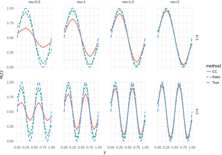
Besides showing the consistency of the regression ratio estimator, we also show that it outperforms the classify and count method in artificial data sets. Specifically, we run the regression ratio estimator using the Nadaraya-Watson kernel estimator and generate data sets under the following specifications:
• Z ∼U(0,1)
• P(Y = 1|S = 1, Z =z) = 0.5
• P(Y = 1|S = 0, Z =z) = 0.5(sin(2zkπ) + 1), fork∈ {1,2}
• X|Y = 0∼N(µ,1) andX|Y = 1∼N(−µ,1), for µ∈ {0.5,1,1.5,2}
• nL=nU = 103
• g(X) is the Bayes classifier, i.e. g(X) =I(X >0)
For each combination of k and µ, 400 independent data sets were generated. Figure
6 presents the average curve fitted for θ(z) using the regression ratio and classify and
count estimators. One can observe that, while for small values of µ the ratio regression
outperforms the classify and count estimator, for large values of µ both estimators are
similar. This occurs because when µis large, the classification problem of determining the
value of Y is easier and both methods perform well. One can also observe from Figure
● ● ● ●
● ● ● ● ●
● ●
● ●
● ● ●
● ●
● ● ●
● ●
● ● ●
● ●
●
● ●
● ● ●
● ●
● ● ●
● ● ●●●●●
●
●
2 0.5
2 1
2 1.5
2 2 1
0.5
1 1
1 1.5
1 2
CC Ratio CC Ratio CC Ratio CC Ratio 0.1
0.2 0.3
0.1 0.2 0.3
method
Error
method CC Ratio
Figure 7: Boxplots of the root mean square deviation in each setting.
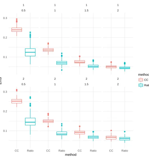
because its fit is generally smoother than the true regression curve. Figure 7 summarizes the mean squared error of each method in each setting. The regression ratio estimator leads to substantial improvements over the classify and count method.
4. Final remarks
We present the ratio estimator for the problem of quantification, show that it is approx-imately minimax under the prior probability shift assumption, and provide an hypothesis test for this assumption. Since the methods in Forman (2006) and Bella et al. (2010) are particular instances of the ratio estimator, it follows that they are also approximately mini-max. The lower bound on the risk that we derive is of independent interest and can be used to investigate the optimality of other quantification methods. We also derive the limiting distribution of the ratio estimator, which allows the derivation of a ratio estimator based on Reproducing Kernel Hilbert Spaces and of confidence intervals for the quantification problem. A simulation study shows that the ratio estimator based on Reproducing Kernel Hilbert spaces is a competitive new alternative.
Besides the above results, we also generalize the ratio estimator to two other scenarios. In the first one, we consider the case in which some labels are available in the target population. The combined estimator uses these labels and the ratio estimator to obtain a larger effective sample size than the ratio estimator. In the second scenario, we consider
the prevalence of positive labels varies according to a new variable, Z. We show that,
unresolved issue is how much it is possible to relax Assumption 6 while still being able to learnθ(Z).
Acknowledgments
This work was partially supported by FAPESP grant 2017/03363-8 and CNPq grant
306943/2017-4. This study was financed in part by the Coordena¸c˜ao de Aperfei¸coamento de Pessoal de
N´ıvel Superior - Brasil (CAPES) - Finance Code 001.
Appendix A. Proofs
Lemma 18 Let XU = (Xu)u∈A0, YU = (Yu)u∈A0, XL= (Xl)l∈A1, and YL= (Yl)l∈A1.
Un-der Assumptions 1 and 2, if θ∼Uniform(0,1), then E[V[θ|XU,XL,YL]] ≥Ω(n−U1). Under the same assumptions, if P(θ = 0.5−n−L1) = P(θ = 0.5 +n−L1) = 0.5, f0 = Bernoulli(0),
α∼Uniform(∗,1)f1|α=Bernoulli(α), then E[V[θ|XU,XL,YL]]≥Ω(n−L1).
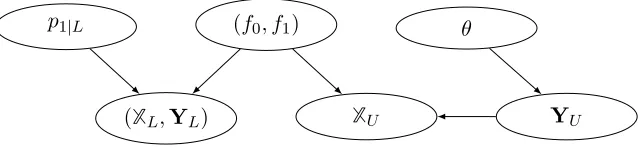
Proof It follows from Assumptions 1 and 2 that the dependency relations between data and parameters can be represented by figure 8.
p1|L
(XL,YL)
(f0, f1)
XU
θ
YU
Figure 8: Dependency relations between data and parameters in the prior shift model.
If θ∼U(0,1), then
E[V[θ|XU,XL,YL]|S1n]≥E[V[θ|XU,XL,YL,YU]|S1n]
=E[V[θ|YU]|S1n] fig. 8
= Ω(n−U1) YU|θ i.i.d. Bernoulli(θ) (4)
Next, let P(θ= 0.5−nL−0.5) = P(θ= 0.5 +n−L0.5) = 0.5, f0 = Bernoulli(0) α∼U(,1)
and f1|α = Bernoulli(α). Define XL,1 = (Xl)l∈A1,1 and note that
f(α|XL,YL)∝αnL,1
¯
Letλ:=θαand observe that, for every λ∈ (0.5 +nL−0.5),0.5−n−L0.5
,
P(θ= 0.5 +nL−0.5|λ,XL,YL) =
fα(λ(0.5 +nL−0.5)−1|XL,YL)
fα(λ(0.5 +nL−0.5)−1|XL,YL) +fα(λ(0.5−nL−0.5)−1|XL,YL)
= 1
1 +
λ
0.5−n−0.5 L
nL,1X¯L,1
1− λ
0.5−n−0.5 L
nL,1(1−¯XL,1)
λ
0.5+n−0.5 L
nL,1X¯L,1
1− λ
0.5+n−0.5 L
nL,1(1−X¯L,1)
eq.5
= 1
1 +1 +n0.45
L −2
nL,1
1− (1−2θα4)n0.5
L +2
nL,1(1−X¯L,1)
λ=θα
(6)
LetγnL :=P(θ= 0.5+n −1
L |λ,XL,YL). Note that nL,1
nL a.s.
→ p1|Land ¯XL,1
a.s.
→ α. Therefore,
since|θ−0.5| ≤nL−0.5, it follows from eq. 6 thatγnL converges a.s. to a quantity between
1 1+exp
−8αp
1|L
1−α
and
1 1+exp
8αp
1|L
1−α
. That is,
E[γnL(1−γnL)|S n
1]≥Ω(1). (7)
Note that ¯XU is sufficient for (θ, α) and ¯XU converges a.s. toλ. Therefore,
E[V[θ|XU,XL,YL]|S1n] =E[V[θ|X¯U,XL,YL]|Sn1] ≥E[V[θ|λ,XL,YL]|Sn1] ≥4n−L1E
γnL(1−γn,L)I λ∈ (0.5 +n −1
L ),0.5−n
−1
L
|S1n
(8)
Since P(λ∈(0.5 +n−L1),0.5−n−L1)≥0.5, it follows from eqs. 7 and 8 that
E[V[θ|XU,XL,YL]|S1n]≥Ω(n−L1) (9)
The proof follows from combining eqs. 4 and 9.
Proof [Theorem 3] We wish to find a lower bound for the minimax risk given a constraint,
F. In order to do so, we use the result that the minimax risk is lower bounded by the
Bayes risk of any Bayes estimator associated to a prior with support in F (Wasserman,
2006; Esteves et al., 2017). Since we consider the squared error loss, the Bayes risk of the
Bayes estimator is E[V[θ|XU,XL,YL]]. Hence, if there exists two priors with support in F
such that the first one satisfies E[V[θ|XU,XL,YL]] ≥ Ω(n−L1) and the second one satisfies
E[V[θ|XU,XL,YL]]≥Ω(n−U1), then we can conclude that the minimax risk is lower bounded
by Ω(max(n−L1, n−U1)). Lemma 18 can be used to determine these priors for the classesFL1,
andFg,k,. The proof forFL1, follows from taking
∗ =in Lemma 18. Next, ifF
g,k,6=∅,
then there exista and bsuch that |g(a)−g(b)| <1. Without loss of generality, leta= 0 and
Lemma 19 For every function, g, under Assumption 3,
θ:=P(Y = 1|S= 0) = E[g(X)|S = 0]−E[g(X)|Y = 0, S = 1]
E[g(X)|Y = 1, S = 1]−E[g(X)|Y = 0, S= 1]
Proof Let f(x) denote the density of X. Note that
g(x)f(x|S = 0) =
1 X
j=0
g(x)f(x|Y =j, S= 0)P(Y =j|S= 0) Law of total prob.
E[g(X)|S = 0] =
1 X
j=0
E[g(X)|Y =j, S = 0]P(Y =j|S= 0) Integration overx
=
1 X
j=0
E[g(X)|Y =j, S = 1]P(Y =j|S= 0) Assumption 3 (10)
Isolating P(Y = 1|S = 0) in equation 10 yields
θ:=P(Y = 1|S= 0) = E[g(X)|S = 0]−E[g(X)|Y = 0, S = 1]
E[g(X)|Y = 1, S = 1]−E[g(X)|Y = 0, S= 1]
Proof [Theorem 6] Follows directly from the definition of θbU R and θbR, and Lemma 19.
Lemma 20 Let Z1 and Z2 be random variables such that E[Z2] 6= 0 and EE[[ZZ12]] ∈ [0,1].
Define T = max0,min1,Z1
Z2
. For every random variable, S, and 1, 2 ∈(0,1).
E
"
T −E[Z1|S] E[Z2|S]
2 S
#
≤ 4(|E[Z1|S]|+1) max (V[Z1|S],V[Z2|S])
min(1,(1−2)4E[Z2|S]4) +
−2
1 V[Z1|S] + (2E[Z2|S])
−2V[Z2|S]
Proof It follows from Taylor’s expansion of Z1
Z2 that there exists Z1,∗ bounded between
E[Z1|S] and Z1, and Z2,∗ betweenE[Z2|S] and Z2 such that
Z1 Z2 =
E[Z1|S]
E[Z2|S]+ 1
Z2,∗
(Z1−E[Z1|S])− Z1,∗
Therefore, by lettingA={|Z1−E[Z1|S]| ≤1,|Z2−E[Z2|S]| ≤2E[Z2|S]}, obtain
E
"
Z1 Z2 −
E[Z1|S]
E[Z2|S]
2
A, S #
P(A|S)
=E
1
Z2,∗
(Z1−E[Z1|S])− Z1,∗
Z22,∗(Z2−E[Z2|S]) !2
A, S
P(A|S)
≤4 max E
"
1
Z22,∗(Z1−E[Z1|S]) 2
A, S #
,E
" Z12,∗
Z24,∗(Z2−E[Z2|S]) 2
A, S #!
P(A|S)
≤
4(|E[Z1|S]|+1) max
E(Z1−E[Z1|S])2A, S
, E
(Z2−E[Z2|S])2
A, S
P(A|S)
min(1,(1−2)4E[Z2|S]4) ≤4(|E[Z1|S]|+1) max (V[Z1|S],V[Z2|S])
min(1,(1−2)4E[Z2|S]4)
(11)
Finally, obtain that
E "
T −E[Z1|S] E[Z2|S]
2 S
#
=E
"
E
"
T− E[Z1|S] E[Z2|S]
2
IA, S
# S
#
≤E
"
Z1 Z2 −
E[Z1|S]
E[Z2|S]
2
A, S #
P(A|S) +P(Ac|S) T,E[Z1]
E[Z2] ∈[0,1]
≤ 4(|E[Z1|S]|+1) max (V[Z1|S],V[Z2|S])
min(1,(1−2)4E[Z2|S]4)
+P(Ac|S) eq. 11
The result follows from applying the union bound and Chebyshev’s inequality to obtain
P(Ac|S)≤P(|Z1−E[Z1|S]|> 1|S) +P(|Z2−E[Z2|S]|> 2E[Z2|S]|S) ≤−12V[Z1|S] + (2E[Z2|S])−2V[Z2|S]
Proof [Theorem 7] Define Z1 =
P
i∈A0g(Xi)
|A0| −
P
i∈A1,0g(Xi)
|A1,0| and also Z2 =
P
i∈A1,1g(Xi)
|A1,1| −
P
i∈A1,0g(Xi)
|A1,0| . Note that
E
P
i∈A0g(Xi) |A0|
Sn1
=E[g(X)|S= 0]
E
" P
i∈A1,jg(Xi)
|A1,j|
Sn1 #
It follows from Lemma 19 that θ= E[Z1|Sn1]
E[Z2|Sn1]. WithT :=θbR= max
0,min
1,Z1
Z2
, obtain
E
b θR−θ
2
Sn1
=E
"
T−E[Z1|S
n
1]
E[Z2|Sn1] 2
Sn1 #
≤ 4(|E[Z1|S
n
1]|+1) max (V[Z1|Sn1],V[Z2|Sn1])
min(1,(1−2)4E[Z2|Sn1]4)
+−12V[Z1|Sn1] + (2E[Z2|Sn1])−2V[Z2|Sn1] Lemma 20
The result follows from observing that, under Fg,K,, E[Z1|S1n] and E[Z2|Sn1] are bounded
by constants, V[Z1|Sn1] =O(max(n
−1
L , n
−1
U )), andV[Z2|Sn1] =O(n
−1
L ).
Proof [Theorem 10] The proof strategy is divided into two parts. The first part consists of proving a joint central limit theorem for the three sample averages that appear in the untrimmed ratio estimator. The second part uses this central limit theorem and the delta method to complete the proof for each case that is considered in the theorem.
The main challenge appears when proving the central limit theorem for the sample aver-ages that appear in the ratio estimator. This occurs since these averaver-ages are not marginally
independent. However, they are independent conditional on the values of Y and S. This
conditional independence can be used to calculate the limiting behavior of the characteristic function of the standardized averages, which completes this part of the proof.
We tidy the proof by using the following notation: µU := E[g(Xi)|Si = 0], σ2U :=
V[g(Xi)|Si= 0],ZU,n:=
√
nU σU
Pn
i=1g(Xi)I(Si=0)
nU −µU
,Zj,n :=
√
nj σj
Pn
i=1g(Xi)I(Si=0,Yi=j)
nj −µj
,
Fi=I(Si = 1)(Yi+ 1), AU ={F1= 0},A0 ={F1= 1}, and A1 ={F1= 2}. Note that
lim
n→∞φZU,n,Z0,n,Z1,n(tU, t0, t1) = limn→∞E
E
exp
X
j∈{U,0,1}
itjZj,n
F1, . . . , Fn
= lim
n→∞E
Y
j∈{U,0,1}
E
exp (itjZj,n)
F1, . . . , Fn
= lim
n→∞E
Y
j∈{U,0,1}
φg(X1)−µj σj
Aj
(tjn−j0.5)
!nj
(12)
It follows from the Central Limit Theorem for i.i.d. random variables that, for every j ∈
{U,0,1}, φng(jX1)−µj σj
Aj
(tjn−j0.5) →exp(−0.5t2j) as nj → ∞. Since nj a.s.
→ ∞, conclude from
eq. 12 and the dominated convergence theorem that
lim
n→∞φZU,n,Z0,n,Z1,n(tU, t0, t1) =
Y
j∈{U,0,1}
exp(−0.5t2j)
and, using1 as the identity matrix, obtain
Assume thatpL6= 0. In this case, since nnL
P
→pL, it follows from eq. 13 that
√ n
Pn
i=1g(Xi)I(Si= 0) nU
−µU,
Pn
i=1g(Xi)I(Si = 0, Yi= 0) n0
−µ0, Pn
i=1g(Xi)I(Si= 0, Yi= 1) n1
−µ1
converges in distribution to N
0, diag σ2
U
1−pL, σ2
0
pLp0|L, σ2
1
pLp1|L
. Since θ = µU−µ0
µ1−µ0 (Lemma
19) and θbU R =
Pn
i=1g(Xi)I(Si=0)
nU −
Pn
i=1g(Xi)I(Si=0,Yi=0)
n0
Pn
i=1g(Xi)I(Si=0,Yi=1)
n1 −
Pn
i=1g(Xi)I(Si=0,Yi=0)
n0
, it follows from the delta method
(Casella and Berger, 2002) that
√
n(θbU R−θ) N 0,
σU2(1−pL)−1
(µ1−µ0)2 +
(µU−µ1)2σ02(pLp0|L)−1
(µ1−µ0)4 +
(µU−µ0)2σ12(pLp1|L)−1
(µ1−µ0)4
!
Since µU = (1−θ)µ0+θµ1 andσ2U = (1−θ)σ20+θσ21+ (µ1−µ0)2θ(1−θ) obtain that √
n(θbU R−θ) N
0,
(1−θ)σ2
0+θσ21+(µ1−µ0)2θ(1−θ)
1−pL +
(1−θ)2σ2 0
pLp0|L + θ2σ2
1
pLp1|L (µ1−µ0)2
Next, assume that pL= 0. Obtain that
p
h(n)(ZU,n−µU)
P
→0 and
p h(n)
√p 0|L
σ0 (Z0,n−µ0), √
p1|L
σ1 (Z1,n−µ1)
N(0,1)
It follows from the delta method and Slutsky’s theorem that
p
h(n)(θbU R−θ) N
0,
(1−θ)2σ2 0
p0|L + θ2σ2
1
p1|L (µ1−µ0)2
The same convergence results hold for θbRsince the derivative of the trimming function
is 1 around θ.
Proof[Theorem 13] It follows from the Representer Theorem (Wahba, 1990) that, for every
g∈ HK,g(x) =Pk∈A1wkK(x,xk). Using this fact, for everyi∈ {0,1},
b µi =
P
j∈A1,ig(xj)
ni
=
P
k∈A1wk P
j∈A1,iK(xj,xk)
ni
=wtmi
b σ2i =
P
j∈A1,i(g(xj)−µbi) 2 ni
=wtΣbiw
Therefore, for everyg∈ HK,
[
MSE(g) = w
tNw
Proof [Proposition 14]
Fg(X)|S=0 =θFg(X)|S=0,Y=1+ (1−θ)Fg(X)|S=0,Y=0
=θFg(X)|S=1,Y=1+ (1−θ)Fg(X)|S=1,Y=0 3
Thus, there exists 0≤p≤1 such thatFg(X)|S=0=pFg(X)|S=1,Y=1+(1−p)Fg(X)|S=1,Y=0.
Proof [Theorem 15]
M SE[θbC] =E
(wbθR+ (1−w)θbL)−θ 2
=E
(w(bθR−θ) + (1−w)(bθL−θ) 2
=w2M SE[θbR] + (1−w)2M SE[θbL] + 2w(1−w)E[(θbR−θ)(θbL−θ)] θbR indep. θbL,E[θbL] =θ
=w2M SE[θbR] + (1−w)2M SE[θbL]
It follows thatM SE[θbC] is minimized by takingw=M SE[θbL]×(M SE[θbL] +M SE[θbR])−1.
Lemma 21 For every function, g, under Assumptions 3 and 6
θ(z) = E[g(X)|S= 0,z]−E[g(X)|Y = 0, S = 1]
E[g(X)|Y = 1, S = 1]−E[g(X)|Y = 0, S = 1]
Proof For every z∈Rdz, Letf(x) denote the density of X. Note that
g(x)f(x|S = 0,z) =
1 X
j=0
g(x)f(x|Y =j, S = 0,z)P(Y =j|S = 0,z) Law of total prob.
E[g(X)|S = 0,z] =
1 X
j=0
E[g(X)|Y =j, S= 0,z]P(Y =j|S = 0,z) Integration overx
=
1 X
j=0
E[g(X)|Y =j, S= 0]P(Y =j|S = 0,z) Assumption 6
=
1 X
j=0
E[g(X)|Y =j, S= 1]P(Y =j|S = 0,z) Assumption 3
(14)
Isolating P(Y = 1|S = 0,z) in equation 14 yields
θ(z) :=P(Y = 1|S = 0,z) = E[g(X)|S= 0,z]−E[g(X)|Y = 0, S= 1]
Proof [Theorem 17] The main difference between this proof and the one of Theorem 7 is that bE[g(X)|S = 0,z] is usually biased for E[g(X)|S = 0,z]. The proof strategy consists of
isolating this bias term from the squared error and then replicating steps which are similar to the ones in Theorem 7.
In order to present the proof in a compact form, some special notation is used. Specifi-cally, h0(z) = E[g(X)|S = 0,z], ˆh0(z) = bE[g(X)|S = 0,z], h1,i = E[g(X)|S = 1, Y = i],
and ˆh1,i = bE[g(X)|S = 1, Y = i]. Using this notation and Definition 16, note that
ˆ
θRR(Z) = max
0,min
1,ˆh0(z)−ˆh1,0 ˆ
h1,1−ˆh1,0
. Therefore,
E
b
θRR(Z)−θ(Z)
2
S1n
=E
"
b
θRR(Z)−
h0(Z)−h1,0 h1,1−h1,0
2
S1n #
Lemma 21
≤O
E
θbRR(Z)−
E[ˆh0(Z)|S1n]−h1,0 h1,1−h1,0
!2
+ E[ˆh0(Z)|S
n
1]−h1,0 h1,1−h1,0
−h0(Z)−h1,0 h1,1−h1,0
!2
S1n
≤O
V[ˆh1,0|Sn1] +V[ˆh1,1|S1n] +V[ˆh0(Z)|S1n] +
E[ˆh0(Z)|S1n]−h0(Z)
2
Lemma 20
=OmaxV[ˆh1,0|S1n],V[ˆh1,1|S1n],E h
(ˆh0(Z)−h0(z))2|S1n i
=Omax
n−L1,E
h
(ˆh0(Z)−h0(z))2|S1n i
Appendix B. Additional Figures
These are additional figures to the experiments of Sections 2.5 and 3.1.
0.1 0.2 0.3 0.4 0.5
Bella CC EM
F
or
man
RKHS Bella CC EM
F
or
man
RKHS Bella CC EM
F
or
man
RKHS Bella CC EM
F
or
man
RKHS Bella CC EM
F
or
man
RKHS
0 1 2 3 4
Method type
Frequency
Figure 10: Number of times in which each specific method presents smaller MSE byθvalues.
cancer candles block spam bank
Bella CC EM
F
or
man
RKHS Bella CC EM
F
or
man
RKHS Bella CC EM
F
or
man
RKHS Bella CC EM
F
or
man
RKHS Bella CC EM
F
or
man
RKHS
0 1 2 3
Method type
Frequency
● ● ● ● ● ● ● ● ● ● ● ● ● ● ● ● ● ● ● ● ● ● ● ● ● ● ● ● ● ● ● ● ● ● ● ● ● ● ● ● ● ● ● ● ● ● ● ● ●● ●● ●● ●● ● ● ● ● ● ● ● ● ● ● ● ● ● ● ● ● ● ● ● ● ● ● ● ● ● ● ● ● ● ● ● ● ● ● ● ● ● ● ● ● ● ● ● ● ● ● ● ● ● ● ● ● ● ● ● ● ● ● ● ● ● ● ● ● ● ● ● ● ● ● ● ● ● ● ● ● ● ● ● ● ● ● ● ● ● ● ● ● ● ● ● ● ● ● ● ● ● ● ● ● ● ● ● ● ● ● ● ● ● ● ● ● ● ● ● ● ● ● ● ● ● ● ● ● ● ● ● ● ● ● ● ● ● ● ● ● ● ● ● ● ● ● ● ● ● ● ● ● ● ● ● ● ● ● ● ● ● ● ● ● ● ● ● ● ● ● ● ● ● ● ● ● ● ● ● ● ● ● ● ● ● ● ● ● ● ● ● ● ● ● ● ● ● ● ● ● ● ● ● ● ● ● ● ● ● ● ● ● ● ● ● ● ● ● ● ● ● ● ● ● ● ● ● ● ● ● ● ● ● ● ● ● ● ● ● ● ● ● ● ● ● ● ● ● ● ● ● ● ● ● ● ● ● ● ● ● ● ● ● ● ● ● ● ● ● ● ● ● ● ● ● ● ● ● ● ● ● ● ● ● ● ● ● ● ● ● ● ● ● ● ● ● ● ● ● ● ●● ●● ●● ●● ● ● ● ● ● ● ● ● ●● ●● ●● ●● ● ● ● ● ● ● ● ● ● ● ● ● ● ● ● ● ● ● ● ● ● ● ● ● ● ● ● ● ● ● ● ● ● ● ● ● ● ● ● ● ● ● ● ● ● ● ● ● ● ● ● ● ● ● ● ● ●● ●● ●● ●● ● ● ● ● ● ● ● ● ●● ●● ●● ●● ● ● ● ● ● ● ● ● ● ● ● ● ● ● ● ● ● ● ● ● ● ● ● ● ● ● ● ● ● ● ● ● ● ● ● ● ● ● ● ● ● ● ● ● ● ● ● ● ● ● ● ● ● ● ● ● ● ● ● ● ● ● ● ● ● ● ● ● ● ● ● ● ●● ●● ●● ●● ● ● ● ● ● ● ● ● ● ● ● ● ● ● ● ● ● ● ● ● ● ● ● ● ● ● ● ● ● ● ● ● ● ● ● ● ● ● ● ● ● ● ● ● ● ● ● ● ● ● ● ● ● ● ● ● ● ● ● ● ● ● ● ● ● ● ● ● ● ● ● ● ● ● ● ● ● ● ● ● ● ● ● ● ● ● ● ● ● ● ● ● ● ● ● ● ● ● ● ● ● ● ● ●
Bella−knn Forman−knn Bella−LR Forman−LR Bella−RF Forman−RF RKHS−Gauss RKHS−Linear
cancer candles b lock spam bank
10 20 30 50 10 20 30 50 10 20 30 50 10 20 30 50 10 20 30 50 10 20 30 50 10 20 30 50 10 20 30 50 0.02 0.04 0.06 0.08 0.02 0.04 0.06 0.08 0.02 0.04 0.06 0.08 0.02 0.04 0.06 0.08 0.02 0.04 0.06 0.08 Labeled size Error
Estimator ●● Combined ● Labeled ● Ratio
Figure 12: Root mean square deviation in logarithmic scale for each data set, method and
estimator by size of the labeled sample and usingθ= 0.1.
References
J. Barranquero, J. D´ıez, and J. J. del Coz. Quantification-oriented learning based on reliable
classifiers. Pattern Recognition, 48(2):591–604, 2015.
A. Bella, C. Ferri, J. Hern´andez-Orallo, and M. J. Ramirez-Quintana. Quantification via
probability estimators. InData Mining (ICDM), 2010 IEEE 10th International
Confer-ence on, pages 737–742. IEEE, 2010.
C. Blake. Uci repository of machine learning databases. http://www. ics. uci. edu/˜
mlearn/MLRepository. html, 1998.
G. Casella and R. L. Berger. Statistical inference, volume 2. Duxbury Pacific Grove, CA,