The Thirty-Third AAAI Conference on Artificial Intelligence (AAAI-19)
Scaling-Up Split-Merge MCMC with Locality Sensitive Sampling (LSS)
Chen Luo, Anshumali Shrivastava
Department of Computer Science, Rice University{cl67, anshumali}@rice.edu
Abstract
Split-Merge MCMC (Monte Carlo Markov Chain) is one of the essential and popular variants of MCMC for problems when an MCMC state consists of an unknown number of components. It is well known that state-of-the-art methods for split-merge MCMC do not scale well. Strategies for rapid mixing requires smart and informative proposals to reduce the rejection rate. However, all known smart proposals involve expensive operations to suggest informative transitions. As a result, the cost of each iteration is prohibitive for massive scale datasets. It is further known that uninformative but com-putationally efficient proposals, such as random split-merge, leads to extremely slow convergence. This tradeoff between mixing time and per update cost seems hard to get around. We leverage some unique properties of weighted MinHash, which is a popular LSH, to design a novel class of split-merge proposals which are significantly more informative than ran-dom sampling but at the same time efficient to compute. Overall, we obtain a superior tradeoff between convergence and per update cost. As a direct consequence, our proposals are around 6X faster than the state-of-the-art sampling meth-ods on two large real datasets KDDCUP and PubMed with several millions of entities and thousands of clusters.
Introduction
Bayesian mixture models are of great interest due to their flexibility in fitting a countably infinite number of compo-nents which can grow with the data (Medvedovic, Yeung, and Bumgarner 2004). The growth of model complexity with the data is also in agreement with modern progress in machine learning over massive datasets. However, the ap-pealing properties of Bayesian modeling come with hard computational challenges. Even with simple mixture mod-els, the mathematical problems associated with training and inference are intractable. As a result, recent research focuses on developing tractable computational techniques. In partic-ular, the use of Markov chain Monte Carlo (MCMC) meth-ods, to sample from the posterior distribution (Andrieu et al. 2003; Nasrabadi 2007; Wang and Blei 2012) is widely prevalent. The practical utility of these methods is illus-trated in several applications including haplotype recon-struction (Eronen, Geerts, and Toivonen 2003), nucleotide
Copyright c2019, Association for the Advancement of Artificial Intelligence (www.aaai.org). All rights reserved.
substitutions (Huelsenbeck and Ronquist 2001),and gene ex-pression (Sharma and Adlakha 2015), etc.
Metropolis-Hastings (MH) (Andrieu et al. 2003) is a fa-vorite class of MCMC methods, which includes several state-of-the-art algorithms that have proven useful in prac-tice. MH is associated with a transition kernel which pro-vides a proposal step. This step is followed by appropriate stochastic acceptance process that ensures detailed balance. A notable example of MH is the Split-Merge MCMC algo-rithm (Jain and Neal 2004; Wang and Russell 2015) which is particularly useful for problems where an MCMC state can be thought of as consisting of a number of components (or clusters). Here as the name suggests, the proposal step com-prises of either a split or a merge. A split move partitions an existing mixture component (or cluster) into two, while a merge move combines two mixture components into one.
In the seminal work of (Jain and Neal 2004), split-merge MCMC procedure was proposed. To illustrate the process, the authors first introduce a random split-merge MCMC, where the split and the merge decision were taken uniformly at random. However, it was also pointed out, in the same pa-per, that due to the random nature of the proposal it was un-likely to lead to a new statex0with higher likelihoodL(x0)
leading to low acceptance. To mitigate the slow progress, the authors then propose the restricted Gibbs split-merge (RGSM). In RGSM, the idea was to use restricted Gibbs sampling to generate proposals with a higher likelihood of acceptance, instead of a random proposal. Thus, a less num-ber of MCMC iterations were sufficient for convergence due to fewer rejections. However, the cost of restricted Gibbs is very high. As a result, even though the iterations are less, each iteration is costly making the overall algorithm slow, especially for large datasets. Our experiments confirm this slow convergence of RGSM.
x0and choose the best ones. This strategy, as expected, en-sures a higher chance of improving the statexwith every proposal. However, from a computational perspective, it is not difficult to see that smart proposalx0obtained after eval-uation of a large number of proposal states, based on the likelihood, is equivalent to evaluating all these states for ac-ceptance/rejection as part of MH (Wang and Russell 2015). As a result, the reduction in the number of iteration is not helpful in obtaining an efficient algorithm. Our experiments show that SDDS also has poor convergence.
Unfortunately, most MCMC methodologies ignore the tradeoff between the number of iteration and computations associated with each iteration. They instead only focus on reducing the number of rejections, which is often achieved by informative proposals with increased per iteration cost. In this paper, we are interested in efficient split-merge MCMC algorithm which leads to overall fast convergence. Thus, re-ducing both is the aim of this work.
Parallelization is Complementary: Due to the signifi-cance of the problem there are several works which try to scale up MCMC by using parallelism. Parallelism is often achieved by running parallel MCMC chains on subsets of data and later merging them (Chang and Fisher III 2013). Since our proposal reduces the overall cost of split-merge MCMC algorithm in general, it will reduce the cost of each of the parallel chains thereby increasing the effectiveness of these parallelisms on MCMC. Thus, existing advances in parallelizing MCMC is complementary to our proposal.
Our Contributions: In this work, we show that it is possible to construct informative proposals without sacri-ficing the per-iteration cost. We leverage a simple observa-tion that while designing proposals we can favor configu-rations where entities similar are likely to be in the same component. We use standard notions of vector similarity such as cosine or Weighted jaccard. To perform such sam-pling efficiently, we capitalize on the recent advances in LSH sampler (Luo and Shrivastava 2018; Spring and Shri-vastava 2017a; Charikar and Siminelakis 2017) that can per-form adaptive sampling based on similarity. This per-forms our first proposal.
Our first proposal leads to around 3x improvements over state-of-the-art methods. However, with similarity driven sampling, computing the Metropolis-Hastings (MH) ratio requires quadratic cost in the size of the cluster being split or merged. This is because while computing the state tran-sition probability, we need to evaluate all possible ways that can lead to the desired split configuration. All these config-urations have different probabilities due to similarity-based adaptive sampling and hence the probability computation is expensive. It appears at first that this cost is unavoidable. Surprisingly, it turns out that there is a rare sweet spot. With Weighted MinHash, we can design a split-merge proposal where the total cost of MH update is only linear in the size of the cluster being split or merged. The possibility is unique to MinHash due to itsk-way generalized collision probabil-ity (Shrivastava and Li 2013). Our proposal and novel exten-sion of MinHash colliexten-sion probability could be of indepen-dent interest in itself.
Overall, our proposed algorithms obtain a sweet tradeoff
between the number of iteration and computational cost per iteration. As a result, we reduce the overall convergence in time, not just in iterations. On two large public datasets, our proposal MinHash Split-Merge (MinSM) significantly outperforms other state-of-the-art split-merge MCMC algo-rithms in convergence speed as measured on wall clock time on the same machine. Our proposed algorithm is around 6x faster than the second best baseline on synthetic datasets as well as realworld datasets without loss in accuracy.
Background
Our work requires bridging Locality Sensitive Sampling with split-merge MCMC algorithm. We briefly review the necessary background.
Locality Sensitive Hashing
Locality-Sensitive Hashing (LSH) is a popular technique for efficient approximate nearest-neighbor search. LSH is a family of functions, such that a function uniformly sampled from this hash family has the property that, under the hash mapping, similar points have a high probability of having the same hash value. More precisely, considerHa family of hash functions mappingRDto a discrete set[0, R−1].
Definition 1 Locality Sensitive Hashing (LSH) FamilyA familyHis called(S0, cS0, u1, u2)-sensitive if for any two pointsx, y ∈ Rd and hchosen uniformly fromHsatisfies
the following:
• ifSim(x, y)≥S0thenP rH(h(x) =h(y))≥u1
• ifSim(x, y)≤cS0thenP rH(h(x) =h(y))≤u2
A collision occurs when the hash values for two data vec-tors are equal, meaning that h(x) = h(y). LSH is a very well studied topic in computer science theory and database literature. There are many well-known LSH families in the literature. Please refer (Gionis et al. 1999) for details.
Locality Sensitive Sampling (LSS) and Unbiased Esti-mators LSH was considered as a black-box algorithm for similarity search and dimensionality reduction. Re-cent research (Spring and Shrivastava 2017a; Charikar and Siminelakis 2017; Luo and Shrivastava 2018; Chen, Shri-vastava, and Steorts 2017; Spring and Shrivastava 2017b) found that LSH can be used for something more subtler but useful. It is a data structure that can be used for ef-ficient dynamically adaptive sampling. We first describe the sampling algorithm of (Spring and Shrivastava 2017a; Charikar and Siminelakis 2017; Luo and Shrivastava 2018; Chen, Shrivastava, and Steorts 2017) and later comment on its properties crucial to our proposal.
one-time linear cost. (2)Sampling Phase:Given a queryq, we collect one bucket from a randomly selected hash table and return a random element from the bucket. If the bucket is empty, we reselect a different hash table again. Keep track of the number of different tablesT probed.
It is not difficult to show that an item returned as a candi-date from a(K, L)-parameterized LSH algorithm is sampled with probability exactly1−(1−pK)L× 1
Size, wherepis the
collision probability of LSH function andSizeis the num-ber of elements in the bucket (Spring and Shrivastava 2017a; Charikar and Siminelakis 2017; Luo and Shrivastava 2018; Chen, Shrivastava, and Steorts 2017). The LSH family de-fines the precise form of p used to build the hash tables. Specifically, whenL = 1andK = 1, the probability re-duced to the collision probability itself (p). Our proposal will heavily rely above observation to design an informative pro-posal distribution.
Weighted (or Generalized) MinHash
Weighted Minwise Hashing is a known LSH for the Weighted Jaccard similarity (Leskovec, Rajaraman, and Ull-man 2014). Given two positive vectorsx, y∈RD,x, y >0,
the (generalized) Weighted Jaccard similarity is defined as
J(x, y) = PD
i=1min{xi,yi}
PD
i=1max{xi,yi}
., where J(x, y)is a frequently
used measure for comparing web-documents (Leskovec, Ra-jaraman, and Ullman 2014), histograms, gene sequences, etc.
Weighted Minwise Hashing (WMH) (or Minwise Sam-pling) generates randomized hash (or fingerprint)h(x), of the given data vectorx≥0, such that for any pair of vectors
xandy, the probability of hash collision (or agreement of hash values) is given byP r(h(x) =h(y)) = Pmin{xi,yi}
Pmax{x
i,yi}.
A unique property of Minwise Hashing is that there is a natural extension ofk-way collision (Shrivastava and Li 2013). In particular, given vectorsx(1), x(2), ..., x(s), the
si-multaneous collision probability is given by:
P r(h(x(1)) =h(x(2)) =...=h(x(s)))
=
PD
j min{x
(1)
j , x
(2)
j , ..., x
(s)
j }
PD
j max{x
(1)
j , x
(2)
j , ..., x
(s)
j }
(1)
Minwise hashing can be extended to negative elements us-ing simple feature transforms (Li 2017), which essentialy doubles the dimentions to 2D. In this paper, MinHash and Weighted MinHash denote the same thing.
Split-Merge MCMC
Split-Merge MCMC (Hughes, Fox, and Sudderth 2012) is useful for dealing with the tasks such as clustering or topic modeling where the number of clusters or components are not known in advance. Split-Merge MCMC is a Metropolis-Hastings algorithm with two main transitions: Split and Merge. During a split, a cluster is partitioned into two com-ponents. On the contrary, a merge takes two components and makes them to one.
During the MCMC inference process, split and merge moves simultaneously change the number of components
and change the assignments of entities to different compo-nents. (Jain and Neal 2004) proposes the first non-trivial Re-stricted Gibbs Split-Merge (RGSM) algorithm, which was later utilized for efficient topic modeling over large datasets in (Wang and Blei 2012).
In (Wang and Russell 2015), the authors presented a surprising argument about information asymmetry. It was shown that both informative split and merge leads to poor acceptance ratio. The author proposed a combination of the smart split with dumb (random) merge and dumb split with smart merge as a remedy. The algorithm was named as Smart-Dumb/Dumb-Smart Split Merge algorithm (SDDS), which was superior to RGSM. To obtain non-trivial smart split (or merge), the authors propose to evaluate a large num-ber of dumb proposals based on the likelihood and select the best. This search process made the proposal very expensive. It is not difficult to see that finding a smart split is compu-tationally not very different from running a chain with sev-eral sequences of dumb (random) splits (Wang and Russell 2015).
LSS based Split-Merge MCMC
Utilizing Similarity Information:In this paper, we make an argument that similarity information, such as cosine sim-ilarity, between different entities is almost always available. For example, in the clustering task, the vector representation of the data is usually easy to get for computing the likeli-hood. Even in an application where we deal with complex entities such as trees, it is not uncommon to have approxi-mate embeddings (Bengio, Weston, and Grangier 2010).
It is natural to believe that similar entities, in terms of co-sine similarity or Jaccard distance, of the underlying vec-tor representation, are more likely to go to the same cluster than non-similar ones. Thus, designing proposals which fa-vor similar entities in the same cluster and dissimilar entities in different clusters is more likely to lead to acceptation than random proposals.
However, the problem is far from being solved. Any similarity based sampling requires computing all pairwise similarity as a prerequisite, which is a quadratic operation
O(n2). Quadratic operations are near-infeasible for large datasets. One critical observation is that with the modern view of LSH as samplers, described preview section, we can get around this quadratic cost and design cheaper non-trivial proposals.
Naive LSS based Proposal Design
This section discusses how LSH can be used for efficient similarity sampling which will lead to an informative pro-posal. In addition, we also want the cost of computing the transition probabilitiesq(x0|x), which is an important com-ponent of the acceptance ratioα(x0|x)(Jain and Neal 2004), to be small. Here,xdenotes the state before split/merge, and
introduce our LSS based proposal design in the rest of this section.
We first create the hash tablesT for sampling. We use Sign Random Projection as the LSH function, thus our no-tion of similarity is cosine (Gionis et al. 1999). It is pointed out that, we can also use other LSH functions when the sim-ilarity notion is different. We pay a one-time linear cost for this preprocessing. Note, we need significantly lessKandL
(both has value 10 in our experiments) compared to what is required for near-neighbor queries as we are only sampling. The sampling is informative for any values ofKandL. For the details of analysis onKandL, please refer (Spring and Shrivastava 2017a).
For our informative proposal, we will need capabilities to do both similarity sampling as well as dissimilarity sampling for merge and split respectively. The similarity sampling is the usual sampling algorithm discussed in previous sections, which ensures that given a queryu, points similar touare more likely to be sampled. Analogously, we also need to sample points that are likely to be dissimilar. With cosine similarity, flipping the sign of the query, i.e., changinguto −uwill automatically do dissimilarity sampling.
Inspired from (Wang and Russell 2015), we also lever-age the information asymmetry and mix smart and dumb moves for better convergence. However, this time our pro-posals will be efficient. At each iteration of MCMC, we start by choosing randomly between an LSH Smart-split/Dumb-merge or an LSH Smart-Smart-split/Dumb-merge/Dumb-split operation. These two operations are defined below:
Naive LSH Smart-split/Dumb-merge LSH based split begins by randomly selecting an elementuin the dataset. Then, we use LSS (Locality-sensitive Sampler) to sample points likely to be dissimilar tou. Thus, we query our data structureT with−uas the query to get another elementv
which is likely far away fromu. Ifuandv belong to the same clusterC, we split the cluster. During the split, we cre-ate two new clustersCu andCv. We assignutoCu andv
toCv. For every element inC, we randomly assign them
to eitherCu orCv. Since we ensure that dissimilar points
uandvare split, this is an informative or smart split. If we finduandvare already in a different cluster, we do a dumb merge: randomly select two components, and merge these two components into one component.
The most important part is that we can precisely compute the probability of the proposed split moveq(x0|x)and the corresponding inverse move probabilityq(x|x0)as follow:
q(x0|x) =
1
2
|Cu|+|Cv|−2
Cu
X
u Cv
X
v
1
n
1− 1−P r(−u, v)KL|Cv∩S−u|
|S−u|
.
=
PCu
u
PCv
v
1
n
1− 1−P r(−u, v)KL|Cv∩S−u|
|S−u|
2|Cu|+|Cv|−2
q(x|x0) = 2
Mx0(Mx0−1)
.
(2)
In the above,nis the number of data point.S−uis the set
of data points that returned by querying inTusing−u, and |S−u|denotes the number of elements inS−u.Mx0denotes
the number of clusters in state x0.C denotes the original component, Cu andCv are the two new components after
split with elementsuandvin them.Kis the number of bits used for hashing, andLis the number of hash tables probed.
P r(−u, v)is the collision probability between−uandv.
Naive LSH Smart-merge/Dumb-split LSH based Merge begins by randomly selecting an elementuin the dataset. Then use LSS to sample from hash tablesT to get another elementvwhich is similar withu. Then, if the mixture com-ponent ofuandvare different, then we do merge operation for the corresponding two mixture component. Ifuandvare in the same components, we do a dumb split: randomly se-lect one cluster, and split this component into two separate components.
We provide the the probability of the merge moveq(x0|x)
and the corresponding inverse probabilityq(x|x0):
q(x0|x) =
Cu
X
u Cv
X
v 1
n
1− 1−P r(u, v)KL|Cv∩Su|
|Su|
,
q(x|x0) = 1 Mx0
(1 2)
|Cu|+|Cv|.
(3)
In the above,Suis the set of data points that returned by
query inT usingu.|Su|denotes the number of elements in
Ss. All the other symbols have the same meaning as before.
P r(u, v)is the collision probability betweenuandv. Notice that, to calculate the transition probabilities in Eq. 2 and Eq. 3, we need to sum over all possibleuandvin the two componentsCuandCv. This could be expensive when
the cluster size is large. In other words, this complexity of this proposal is quadratic to the size of the cluster.
The quadratic cost seems unavoidable. LSH does simi-larity based sampling. Thus, we can sample pairs uandv
in adaptive fashion efficiently. A split of clusterC intoCu
andCv can happen because of any two elementsx ∈ Cu
andy∈Cvbeing samples. As a result, the transition
proba-bility requires accumulating non-uniform probabilities of all possible combinations, making it quadratic to compute. On the other hand if every pair has same probability then the proposal is random. Overall, it seems hopeless to split the cluster adaptively and at the same time get the probability of split linear in the size of cluster.
It turns out, surprisingly, that a very unique design of pro-posal that satisfies our wishlist. It is the unique mathemat-ical properties of MinHash and a novel generalization of its k-way collision probability that makes this possible. In the next section, we will introduce the method of usek-way minhash for scaling up MCMC (Shrivastava and Li 2013).
MinSM: MinHash based Split-Merge MCMC
Ideally, after identifyinguwe should split so that all the ele-ments similar tougoes toCuand rest goes toCv. This will
probability of configuration under LSH would be computa-tionally expensive, as LSH sampling is correlated and the expressions are contrived as we introduced before.
We next show that MinHash with a very specific design exactly achieves this otherwise impossible and ideal state with the cost of evaluating the transition probability linear in the size of the cluster. A unique property of MinHash is that we can compute, in closed form and linear cost, the proba-bility of collision of a set of points of any size≥ 2. Such computation is not possible with any other know LSH in-cluding the popular random projections (Gionis et al. 1999). We provide a novel extension of the collision probabil-ity of MinHash to also include the probabilprobabil-ity of collision with a given set and no collision with another given set (See Equation 1). It is surprising that despite many non-trivial correlations, the final probability expression is very simple and only requires linear computations. As a result, we can directly get the split of a cluster into two sets (or clusters) and at the same time compute the transition probability. The novel design and analysis of Minhash, presented here, could be of independent interest in itself.
MinHash Smart-split/Dumb-merge MinHash based split begins by flipping a coin to randomly choose from the action of Smart-split or Dumb merge.
The LSH smart-split begins by randomly selecting an ele-mentuin the dataset. Then, we use LSS (Locality-sensitive Sampler) to sample a set of points that are likely to be simi-lar toufromT, i.e., queryT withu. Here we use Weighted MinHash as the LSH andK= 1is necessary.K≥1makes the probability computations out of reach. Instead of sam-pling a point from the bucket, as we do with LSS, we just report the whole bucket as the set. Let us denote this sam-pled set as Su. We now split the componentCu into two
components: Cu∩Su, Cu−Su. If the action is a dumb
merge, then we randomly select two components and merge these two components into one component.
Given a new statex0, and the corresponding old statex, we can precisely compute the probability of the proposed split move q(x0|x) and the corresponding inverse move probabilityq(x|x0)as follow:
Definepas the probability of agreement of weighted min-hash ofuwith all of the data point in the queried setSu. The
known theory (Gionis et al. 1999) says that the expression ofpis given by Equation 1. However, we want something more, we want all elements ofSu to collide withuin the
bucket and anything inCu−Suto not collide. DefineP rob
as the probability of agreement of weighted minhash ofu
with all ofSuand none of the data point inCu−Su. It turns
our that we can calculate this probability exactly as:
P rob=
P2D
j max{0,(x j
min−x
j
max)}
P2D
j x j all
, (4)
where xjmin = minx∈Cu∩Su{xj}, x
j
max =
maxx∈C−Su{xj}andx
j
all= maxx∈Cu{xj}
When we only useK= 1Minhash, then the correspond-ing proposal distribution is shown as follow:
q(x0|x) = |Su|
n ×P rob. (5)
a
b
c
f
e
d
g
𝑋𝑋
1𝑋𝑋
2𝑋𝑋
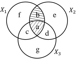
3Figure 1: Three way Minwise Hashing.
Here, we give an illustration of the proof. Consider Fig-ure 1. Let’s start with vanilla MinHash over sets and the ar-guments will naturally extend to weighted versions. Given
X1,X2andX3. We want the probability that the MinHash
ofX1andX2collide but not ofX3. From the theory of con-sistent sampling (Shrivastava and Li 2013; Shrivastava 2016; Manasse, McSherry, and Talwar 2010). This will happen if we sample fromband the possibility is the union. Thus the probability isa+b+c+db+e+f+g = |X|X1∩X2|−|X3|
1∪X2∪X3| which is
es-sentially we want the minimum of|X1∪X2∪X3| to be
sampled from the intersection ofX1 andX2and not from
X3. That is the only way the MinHash ofX1andX2 will agree but not ofX3. This argument can be naturally exten-dend if we wantX1, X2, ..., Xhto have same minhash and
notY1, Y2, ..., Yg, the probability can be written as:
max{0,|X1∩X2∩...∩Xh| − |Y1∪Y2∪...∪Yg|}
|X1∪X2∪...∪Xh∪Y1∪Y2∪...∪Yg|
.
Now for weighted sets (non-binary), we can replace in-tersection with minimum and unions with max leading to the desired expression, which is due to the seminal works in consistent weighted sampling a strict generalization of MinHash. See (Shrivastava and Li 2013; Shrivastava 2016; Manasse, McSherry, and Talwar 2010) for details. Also us-ing (Leskovec, Rajaraman, and Ullman 2014) we can extend it to negative weights as well using simple feature transfor-mation.
It should be noted that this expression only requires cost linear in the size of the cluster Cu being split. With this
value ofP rob, the corresponding transition probability for the split move is:
q(x0|x) = |Su|
n ×P rob, q(x|x
0) = 2
Mx0(Mx0−1)
. (6)
In the above,nis the number of data point.Suis the set of
data points that returned by querying inT usingu, and|Su|
denotes the number of elements inSu.Dis the dimension
of the data.Mx0 denotes the number of clusters in statex0.
Minhash Smart-merge/Dumb-split The proposed smart-merge begins by randomly selecting a centeruin the dataset. Then, we use LSS (Locality-sensitive Sampler) to sample a centervthat are likely to be similar tou. Then we merge the componentCuandCvto one component.
If the action is a dumb split: randomly select one clus-ter, and split this component into two separate components uniformly.
Given a new statex0, and the corresponding old statex. We provide the probability of the merge moveq(x0|x)and the corresponding inverse probabilityq(x|x0)as follow:
q(x0|x) = 1
Mx
P2D
j min{uj, vj}
P2D
j max{uj, vj}
1
|Su|
,
q(x|x0) = 1
Mx0 (1
2)
|Cu|+|Cv|.
(7)
In the above,Suis the set of data points that returned by
the query in hash tableT usingu.|Su|denotes the number
of elements inSu.uj denotesj-th feature of the data point
u. All the other symbols have the same meaning as before. As we introduced before, our proposed algorithm be-longs to the general framework of metroplis-hastings algo-rithm (Andrieu et al. 2003). After each split/merge move, we need to calculate the acceptance rateα(x0|x)for this move:
α(x0|x) = min{1,LL((xx0))qq((xx0||xx0))}, wherex0 is the proposed
new state,xis the previous state,q(x0|x)here is the designed proposal distribution, and it can be calculated as introduced in previous sections.L(x)is the likelihood value of the state
x.
The likelihood of the data is generally in the form of
L(x) = Q
Dpj(ei), where pj(ei) is the probability of
ei ∈Din it’s corresponding componentCj.Ddenotes the
total dataset. In the split merge MCMC, only the compo-nents that being split/merged will change of the likelihood value. So, that the ratio LL((xx0)) is cheap to compute, since all the probability of unchanged data will be canceled.
Empirical Study
In this section, we demonstrate the advantage of our pro-posed models by applying it to the Gaussian Mixture model inference and compare it with state-of-the-art sampling methods.
Gaussian Mixture Model
We briefly review the Gaussian Mixture Model. A Gaus-sian mixture density is a weighted sum of component den-sities. For aM-class clustering task, we could have a set of GMMs associated with each cluster. For a D-dimensional feature vector denoted asx, the mixture density is defined as
p(x) =PM
i=1wipi(x), wherewi, i= 1, ..., M are the
mix-ture weights which satisfy the constraint thatPM
i = 1and
wi ≥0. The mixture density is a weighted linear
combina-tion of componentMuni-model Gaussian density functions
pi(x), i= 1, ..., M. The Gaussian mixture density is
param-eterized by the mixture weights, mean vectors, and covari-ance vectors from all components densities.
For a GMM-based clustering task, the goal of the model training is to estimate the parameters of the GMM so that the Gaussian mixture density can best match the distribu-tion of the training feature vectors. Estimating the parame-ters of the GMM using the expectation-maximization (EM) algorithm (Nasrabadi 2007) is popular. However, in most of the real world applications, the number of clustersM is not known, which is required by the EM algorithm. On the other hand, Split-Merge based MCMC algorithms are used for in-ference whenM is unknown, which is also the focus of this paper. We therefore only compare our proposal LSHSM and other state-of-the-art split-merge algorithms on GMM clus-tering which does not require the prior knowledge of the number of clusters.
Experimental Setup
Competing Algorithms:We compare following four split-merge MCMC sampling algorithm on GMM with an un-known number of clusters:RGSM:Restricted Gibbs split-merge MCMC algorithm (Jain and Neal 2004) is considered as one of the state-of-the-art sampling algorithm. SDDS: Smart-Dumb/Dumb-Smart Split Merge algorithm (Wang and Russell 2015). LSHSM: The Naive version of LSH based Split Merge algorithm by using Sign Random Pro-jection. In the LSHSM method, we use fixedK = 10and
L = 10 for all the dataset. We fix the hashing scheme to be signed random projection. MinSM:LSH based split merge algorithm is the proposed method in this paper. In the MinSM method, we use fixedK = 1andL= 1for all the dataset.
0 2 4 6 8 10
CPU Execution Time(h)
0 2K 4K 6K 8K 10K 12K
Likelihood
LSHSM RGSM SDDS MinSM
(a) KDDCUP Dataset
0 5K 10K 15K
Number of Iterations
0 0.5K 1K 1.5K 2K 3K 3.5K
Likelihood LSHSMRGSM
SDDS MinSM
(b) KDDCUP Dataset
0 0.5K 1K 1.5K 2K 2.5K
CPU Execution Time(s)
0 0.5K 1K 1.5K 2K 2.5K 3K
Likelihood LSHSM RGSM SDDS MinSM
(c) PubMed Dataset
0 2M 4M 6M 8M
Number of Iterations
0 2K 4K 6K 8K 10K 12K
Likelihood LSHSMRGSM
SDDS MinSM
(d) PubMed Dataset
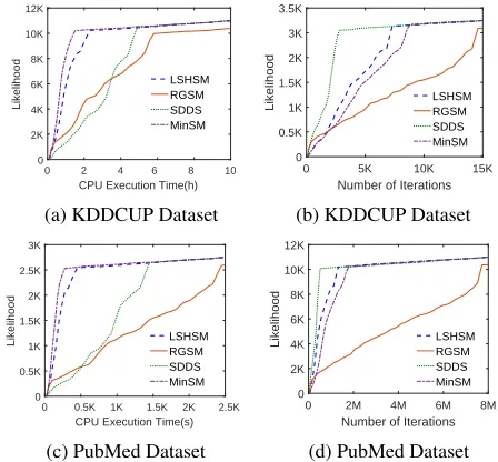
Figure 2: The time and iteration wise comparison of the likelihood for difference methods on the two real dataset. It is obviously that our proposed MinSM algorithm can be at least6times faster than the state of the art algorithms in the real large dataset.
0 1000 2000 3000 4000 5000
Number of Iterations
0 2 4 6 8 10 12
Likelihood
LSHSM RGSM SDDS MinSM
(a) S1 dataset
0 20K 40K 60K 80K 100K
Number of Iterations
0 25 50 75 100 125 150
Likelihood
LSHSM RGSM SDDS MinSM
(b) S2 dataset
0 100K 200K 300K 400K 500K
Number of Iterations
0 150 300 450 600 750 900
Likelihood
LSHSM RGSM SDDS MinSM
(c) S3 Dataset
0 1 2 3 4 5 CPU Execution Time(s) 0
2 4 6 8 10 12
Likelihood
LSHSM RGSM SDDS MinSM
(d) S1 dataset
0 5 10 15 20 25
CPU Execution Time(s)
0 25 50 75 100 125 150
Likelihood
LSHSM RGSM SDDS MinSM
(e) S2 dataset
0 100 200 300 400 500
CPU Execution Time(s)
0 150 300 450 600 750 900
Likelihood
LSHSM RGSM SDDS MinSM
(f) S3 dataset
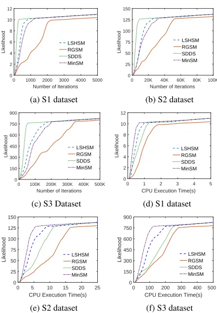
Figure 3: The time and iteration wise comparison of the likelihood for difference methods on the Synthetic Dataset. MinSM outperforms the other baselines by a large margin. It is also clear that requiring less iteration does not mean faster convergence.
PubMed.KDDCUPdata was used in the KDD Cup 2004 data mining competition. It contains 145751 data point. The dimensionality of the dataset is 74. We have 2000
ground truth cluster labels for this dataset.1 ThePubMed
abstraction dataset contains 8200000 abstractions that ex-tracted from the PubMed2. All the documents represented
as the bag-of-words representation. In the data set, we have
141043, different words. This data set is ideal for document clustering or topic modeling.
Synthetic data is a standard way of testing GMM models (Nasrabadi 2007). So, in this paper, we also use synthetic datasets as a sanity check to evaluate the performance of different methods. The process of generating the synthetic dataset is as follow: Randomly generatekdifferent Gaussian distributions (with different corresponding mean and vari-ance). We fix thek= 10in our experiment. Then based on the randomly generated Gaussian distributions, we generate a set of data points for each Gaussian distribution. Here we fix the dimensionality of each data point to25. In this
exper-1
https://cs.joensuu.fi/sipu/datasets/
2
www.pubmed.gov
Table 1: Clustering Accuracy for Different Methods
Methods Metric S1 S2 S3 KDD Pub RGSM NMI 0.96 0.93 0.88 0.74 0.63 Accuracy 0.95 0.92 0.87 0.68 0.62 SDDS NMI 0.97 0.96 0.95 0.86 0.80 Accuracy 0.98 0.97 0.94 0.85 0.77 LSHSM NMI 0.96 0.95 0.96 0.84 0.77 Accuracy 0.97 0.94 0.96 0.83 0.75 MinSM NMI 0.96 0.94 0.96 0.83 0.75 Accuracy 0.97 0.94 0.97 0.84 0.74
iment, we generate three sythntic dataset with different size (e.g.100,1000,10000). We name the three synthetic dataset asS1,S2,S3.
Speed Comparison and Analysis
We first plot the evolution of likelihood both as a function of iterations as well as the time of all the three competing meth-ods. The evolution of likelihood and time with iterations on two real-world data is shown in Fig. 2. The result on three synthetic data set is shown in Fig. 3.
We can see a consistent trend in the evolution of likeli-hood, which holds true for both simulated as well as real datasets. First of all, RGSM consistently performs poorly and requires both more iterations as well as time. This demonstrate that the need of combining smart and dumb moves for faster convergence made in (Wang and Russell 2015) is necessary. RGSM does not use it and hence leads to poor, even iteration wise, convergence.
SDDS seems to do quite well, compared to our proposed LSHSM when we look at iteration wise convergence. How-ever, when we look at the time, the picture is completely changed. MinSM is significantly faster than SDDS, even if the convergence is slower iteration wise. This is not sur-prising because the per-iteration cost of MinSM is orders of magnitude less than SDDS. SDDS hides the computa-tions inside the iteration by evaluating every possible state in each iteration, based on likelihood, is equivalent to sev-eral random iterations combined. Such costly evaluation per iteration can give a false impressing of less iteration.
It is clear from the plots that merely comparing iterations and acceptance ratio can give a false impression of supe-riority. Time wise comparison is a legitimate comparison of overall computational efficiency. Clearly, MinSM outper-forms the other baselines by a large margin.
Clustering Accuracy Comparison
To evaluate the clustering performance of different algo-rithms, we use two widely used measures (Accuracy and NMI (Nasrabadi 2007)).Normalized Mutual Information (NMI)(Nasrabadi 2007) is widely used for measuring the performance of clustering algorithms. It can be calculated asN M I(C, C0) = √I(C;C0)
H(C)H(C0),whereH(C)andH(C 0)
correct cluster, is defined asAccuracy=
Pk i=1ai
n ,whereai
is the number of data objects clustered to its corresponding true cluster,kis the number of cluster andnis the number of data objects.
Table 1 shows the clustering accuracy of different com-peting methods. We can see that the MinSM, LSHSM and SDDS are much more accurate than RGSM. This observa-tion is in agreement with the likelihood plots. On the other hand, the accuracy difference between MinSM, LSHSM and SDDS is negligible. This small difference is due to the mis-match between the likelihood value and clustering accuracy. It should be noted that the difference is small for SDSS and MinSM variants because both achieved the same likelihood value. For the Random Split merge with the worse likeli-hood, the difference is huge, indicating the clustering results does correlate with likelihood values except for minor vari-ations.
Conclusion
The Split-Merge MCMC (Monte Carlo Markov Chain) is one of the essential and popular variants of MCMC for problems with an unknown number of components. It is a well known that the inference process of SplitMerge MCMC is computational expensive which is not applicable for the large-scale dataset. Existing approaches that try to speed up the split-merge MCMC are stuck in a computational chicken-and-egg loop problem.
In this paper, we proposed MinSM, accelerating Split Merge MCMC via weighted Minhash. The new splitmerge MCMC has constant time update, and at the same time the proposal is informative and needs significantly fewer itera-tions than random split-merge. Overall, we obtain a sweet tradeoff between convergence and per update cost. Exper-iments with Gaussian Mixture Model on two real-world datasets demonstrate much faster convergence and better scaling to large datasets.
Acknowledgement
This work was supported by National Science Foundation IIS-1652131, BIGDATA-1838177, RI-1718478, AFOSR-YIP FA9550-18-1-0152, Amazon Research Award, ONR BRC grant on Randomized Numerical Linear Algebra.
References
Andrieu, C.; De Freitas, N.; Doucet, A.; and Jordan, M. I. 2003. An introduction to mcmc for machine learning. Machine learning
50(1-2):5–43.
Bengio, S.; Weston, J.; and Grangier, D. 2010. Label embedding trees for large multi-class tasks. InAdvances in Neural Information Processing Systems, 163–171.
Chang, J., and Fisher III, J. W. 2013. Parallel sampling of dp mixture models using sub-cluster splits. InAdvances in Neural Information Processing Systems, 620–628.
Charikar, M., and Siminelakis, P. 2017. Hashing-based-estimators for kernel density in high dimensions. FOCS.
Chen, B.; Shrivastava, A.; and Steorts, R. C. 2017. Unique entity estimation with application to the syrian conflict. arXiv preprint arXiv:1710.02690.
Eronen, L.; Geerts, F.; and Toivonen, H. 2003. A markov chain approach to reconstruction of long haplotypes. InBiocomputing 2004. World Scientific. 104–115.
Gionis, A.; Indyk, P.; Motwani, R.; et al. 1999. Similarity search in high dimensions via hashing. InVLDB, volume 99, 518–529. Huelsenbeck, J. P., and Ronquist, F. 2001. Mrbayes: Bayesian inference of phylogenetic trees. Bioinformatics17(8):754–755. Hughes, M. C.; Fox, E.; and Sudderth, E. B. 2012. Effective split-merge monte carlo methods for nonparametric models of sequen-tial data. InAdvances in neural information processing systems, 1295–1303.
Jain, S., and Neal, R. M. 2004. A split-merge markov chain monte carlo procedure for the dirichlet process mixture model.Journal of Computational and Graphical Statistics13(1):158–182.
Leskovec, J.; Rajaraman, A.; and Ullman, J. D. 2014. Mining of massive datasets. Cambridge university press.
Li, P. 2017. Linearized gmm kernels and normalized random
fourier features. InProceedings of the 23rd ACM SIGKDD Inter-national Conference on Knowledge Discovery and Data Mining, 315–324. ACM.
Luo, C., and Shrivastava, A. 2018. Arrays of (locality-sensitive) count estimators (ace): Anomaly detection on the edge. In Proceed-ings of the 2018 World Wide Web Conference, WWW’18, 1439– 1448.
Manasse, M.; McSherry, F.; and Talwar, K. 2010. Consistent weighted sampling.Unpublished technical report) http://research. microsoft. com/en-us/people/manasse2.
Medvedovic, M.; Yeung, K. Y.; and Bumgarner, R. E. 2004.
Bayesian mixture model based clustering of replicated microarray data.Bioinformatics20(8):1222–1232.
Nasrabadi, N. M. 2007. Pattern recognition and machine learning.
Journal of electronic imaging16(4):049901.
Sharma, A., and Adlakha, N. 2015. A computational model to study the concentrations of dna, mrna and proteins in a growing cell.Journal of Medical Imaging and Health Informatics5(5):945– 950.
Shrivastava, A., and Li, P. 2013. Beyond pairwise: Provably fast algorithms for approximatek-way similarity search. InAdvances in Neural Information Processing Systems, 791–799.
Shrivastava, A. 2016. Simple and efficient weighted minwise hash-ing. InAdvances in Neural Information Processing Systems, 1498– 1506.
Spring, R., and Shrivastava, A. 2017a. A new unbiased and
efficient class of lsh-based samplers and estimators for parti-tion funcparti-tion computaparti-tion in log-linear models. arXiv preprint arXiv:1703.05160.
Spring, R., and Shrivastava, A. 2017b. Scalable and sustainable deep learning via randomized hashing. InProceedings of the 23rd ACM SIGKDD International Conference on Knowledge Discovery and Data Mining, 445–454. ACM.