Finite Difference Method For Solving Fuzzy
Linear Boundary Value Problems
Rasha H.Ibraheem
Department of Mathematics , College of Basic Education ,Al- mustansiriyah University, Baghdad- Iraq.
ABSTRACT
:
In this paper, the Finite Difference method is considered to solve the nonhomogeneous for Second order fuzzy boundary value problems, In which the fuzziness appeared together in the boundary conditions and in the nonhomogeneous term of the differential equation. The method of solution depends on transforming the fuzzy problem to equivalent crisp problems using the concept of α-level sets.
KEYWORDS: the Finite Difference Method; Fuzzy sets; α-level sets; second order fuzzy boundary value problems
.
I. INTRODUCTION
A fuzzy set theory had been introduced by Zadeh in 1965, in which, Zadeh's original definition of fuzzy set is as follows: A fuzzy set is a class of objects with a continuum grades of membership, such a set is characterized by a membership or characteristic function which assigns to each object a grade of membership ranging between zero and one, [1].
Kandel [5] applied the concept of fuzzy differential equations to the analysis of fuzzy dynamical problems, but the boundary value problems was treated, rigorously by Lakshmikantham, V., Murty, K. N. and Turner, J. in 2001, [8]. Henderon, J. and Peterson, A. in 2004 obtained a theorem of the existence and uniqueness of solutions for the boundary value problems of fuzzy differential equations.
Pearson in 1997 [3], introduced the analytical method for solving linear system of fuzzy differential equations.
In this paper, the Finite Difference method is applied to solve the second order fuzzy boundary value problems. This method we will present here have better stability characteristics, but generally require more computations to obtain a pre-specified accuracy.
The purpose of this paper is involving finite differences for solving boundary value problems consists of replacing each of the derivatives in the differential equation by an appropriate difference approximation. The difference equation is generally chosen so that a certain order of truncation error is maintained [9]. Consider the following second order fuzzy boundary value problem
,
The structure of the paper include the following: in section 2, we provide some important definitions and basic results to be used in this paper. in section 3 we present Finite Difference Method . In section 4, we illustrate proposed method by numerical example.
II. FUZZY SETS:
In this section, we shall present some basic definitions of fuzzy sets including the definition of fuzzy numbers and fuzzy functions
.
Definition (1), [6]:
Let X be any set of elements. A fuzzy set is characterized by a membership function : X [0, 1], and may be written as the set of points
Definition (2), [4]:
The crisp set of elements that belong to the set at least to the degree is called the weak -level set (or weak -cut), and is defined by:
Definition (3),[7]:
A fuzzy subset of a universal space X is convex if and only if the sets are convex, . Or equivalently, we can define convex fuzzy set directly by using its membership function to satisfy:
For all and
Definition (4),[2]:
A fuzzy number Is a convex normalized fuzzy set Of the real line R, such that: 1. There exists exactly one ∈R, with ( Is called the mean value of ). 2. Is piecewise continuous
Now, in applications, the representation a fuzzy number in terms of its membership function is so difficult to use, therefore two approaches are given for representing the fuzzy number in terms of its -level sets, as in the following remark:
Remark (1):
A fuzzy number may be uniquely represented in terms of its --level sets, as the following closed intervals of the real line:
or
Where is the mean value of and α∈ [0, 1]. This fuzzy number may be written as
where refers to the greatest lower bound of and to the least upper bound of .
Remark (2):
Similar to the second approach given in remark (1), one can fuzzyfy any crisp or nonfuzzy function f, by letting:
, , , α∈ (0, 1]
and hence the fuzzy function in terms of its α -levels is given by .
III. FINITE DIFFERENCE METHOD FOR SOLVING FUZZY LINEAR BOUNDARY VALUE PROBLEMS:
In this paper, we consider the finite difference method for the linear second order fuzzy BVP: ………(1)
,
requires that the difference approximations be used for approximating both y and y. To accomplish this, we select an integer N > 0 and divide the interval [a, b] into N + 1 equal subintervals, whose end points are the mesh points , for i 0, 1, …, N + 1; where . Choosing the constant h in this manner will facilitate the application of a matrix algorithm, which in this form will require of solving a linear system that involves NN matrix.
In this case, the parametric equations related to eq.(1) are given by:
With boundary conditions:
, and and
with boundary conditions:
Expanding y in a third-degree Taylor polynomial about xi evaluated at and , and assuming
y
C4[ ], we have:
for some point i+, < i+ < , and:
for some point i, < i < .
If these equations are added together, the terms involving
y
(xi) andy
(xi) are eliminated, and a simple algebraic manipulation gives:The intermediate value theorem can be used to simplify the last equation even further:
... (3)
for some pointi, < i < .
Equation (3) is called the central difference formula for .
A central-difference formula for
y
( ) can be obtained in a similar manner, resulting in:... (4)
for some i, where < i < .
The use of these central-difference formulas in eq.(2) results in the equation:
A finite difference method wit truncation error of order o(h2) results by using this equation together with the boundary conditions and , to define:
, and And
……….(5)
for each i 1, 2, …, N. In the form we will consider eq.(5) is rewritten as:
where:
2
1 1
2
2 2 2
2
i i
n 1 2
n n
h
2
h q(x )
1
p(x )
0
0
2
h
h
1
p(x )
2
h q(x )
1
p(x )
2
2
h
h
0
1
p(x )
2
h q(x )
1
p(xi)
A
2
2
0
h
1
p(x
)
2
h
0
0
1
p(x )
2
h q(x )
2
y
1
2
i
N 1
N
y
y
y
y
y
, b
2
1 1 0
2 2
2 i
2
N 1
2
N N N 1
h
h r(x )
1
p(x ) y
2
h r(x )
h r(x )
h r(x
)
h
h r(x )
1
p(x ) y
2
IV.Illustrative Example
Consider the fuzzy BVP:
………..…(7)
, …………...………..………(8)
For this example, we will use N 9, so that h 0.1. In this case, the parametric equations related to eqs.(7) and (8), are:
With boundary conditions:
, and which is a non fuzzy BVP.
By using eq.(4), we get:
………..(9)
For each i 1, 2, …, 9.
In this form, we will consider eq.(9) which can be written as:
x
2i h2and the resulting system of algebraic equations may be expressed in the triadiagonal 99 matrix form: ... (10) Where: 2 2 1 1 2 2
2 2 2
2 2
3 3 3
2 2
4 4 4
2 2
5 5 5
2 2
6 6 6
2 2
7 7 7
2 2
8 8
2 h
2 h 1 0 0 0 0 0 0 0
x x
h 2 h
1 2 h 1 0 0 0 0 0 0
x x x
h 2 h
0 1 2 h 1 0 0 0 0 0
x x x
h 2 h
0 0 1 2 h 1 0 0 0 0
x x x
h 2 h
0 0 0 1 2 h 1 0 0 0
A
x x x
h 2 h
0 0 0 0 1 2 h 1 0 0
x x x
h 2 h
0 0 0 0 0 1 2 h 1 0
x x x
h 2
0 0 0 0 0 0 1 2 h
x x 8 2 2 9 9 h 1 x h 2
0 0 0 0 0 0 0 1 2 h
x x
2 2 1 11 2 2
2 2 2 2 3 3 2 2 4 4 2 2 5 5 2 2 6 6
7 2 2
7
8 2 2
8 9 2 2 9 9
h
h x
1
1
1
x
y
h x
y
h x
y
h x
y
y
y
, b
h x
y
h x
y
h x
y
h x
y
h
h x
1
2
1
We can carry similar calculations as it is followed for lower case of solution and find the upper case of solution from the following system of algebraic equations:
... (11) Where 2 2 1 1 2 2
2 2 2
2 2
3 3 3
2 2
4 4 4
2 2
5 5 5
2 2
6 6 6
2 2
7 7 7
2 2
8 8
2 h
2 h 1 0 0 0 0 0 0 0
x x
h 2 h
1 2 h 1 0 0 0 0 0 0
x x x
h 2 h
0 1 2 h 1 0 0 0 0 0
x x x
h 2 h
0 0 1 2 h 1 0 0 0 0
x x x
h 2 h
0 0 0 1 2 h 1 0 0 0
A
x x x
h 2 h
0 0 0 0 1 2 h 1 0 0
x x x
h 2 h
0 0 0 0 0 1 2 h 1 0
x x x
h 2
0 0 0 0 0 0 1 2 h
x x 8 2 2 9 9 h 1 x h 2
0 0 0 0 0 0 0 1 2 h
x x
2 2 1 11 2 2
2
2 2 2
3 3 2 2 4 4 2 2 5 5 2 2 6 6
7 2 2
7
8 2 2
8 9 2 2 9 9
h
h x
1
1
1
x
y
h x
y
h x
y
h x
y
y
y
, b
h x
y
h x
y
h x
y
h x
y
h
h x
1
2
1
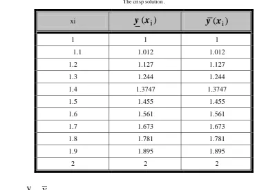
TABLE 1
The crisp solution .
xi
y x
(
i)
y x
(
i)
1 1 1
1.1 1.012 1.012
1.2 1.127 1.127
1.3 1.244 1.244
1.4 1.3747 1.3747
1.5 1.455 1.455
1.6 1.561 1.561
1.7 1.673 1.673
1.8 1.781 1.781
1.9 1.895 1.895
2 2 2
Hence y [
y
,y
] is the solution of the original fuzzy BVP.V. CONCLUSIONS:
From the present study of this paper, we may conclude the following:
1. The accuracy of the results may be checked with α = 1, in which the upper and lower
solutions must be equal.
2. The crisp solution or the solution of the nonfuzzy boundary value problem is obtained from
the fuzzy solution by setting α = 1, and therefore fuzzy boundary value problems may be
considered as a generalization to the nonfuzzy boundary value problems.
3. The finite difference method proved its validity and accurate results in solving fuzzy
boundary value problems.
AKNOWLEDGMENTS The authors would like to thank Mustansiriyah University
(WWW.uomustansiriyah.edu.iq) Baghdad –Iraq for its support in the present work.
V. REFERENCES
[1] Pal S. K. and Majumder D.K Fuzzy Mathematical Approach to Pattern Recognition , John Wiley and sons, Inc., New York, 1986.
[2] Dubois, D. and Prade, H., Fuzzy Sets and Systems; Theory and Applications , Academic Press, Inc., 1988.
[3] Pearson, D. W.: “A Property of Linear Fuzzy Differential Equations”, Appl. Math. Lett., Vol.10, No.3, 1997, pp.99-103. [4] Zimmerman, H. J., "Fuzzy Set Theory and Its Applications", Kluwer-Nijhcff Publishing, USA, 1988.
[5] Kandel A., Fuzzy Mathematical Techniques with Applications , Addison Wesley Publishing Company, Inc., 1986.
[6] Zadeh, L. A., "Fuzzy Sets", Information Control, 8 (1965), 338-353.
[7] Yan, J., Ryan, M. and Power, J., Using Fuzzy Logic: Towards Intelligent Systems , Prentice Hall, Inc., 1994.
[8] Al-Adhami R. H., "Numerical Solution of Fuzzy Boundary Value Problems", M.Sc. Thesis, College of Science, Al-Nahrain University, 2007.