Download Download PDF

(1)

ANALYSING THE IMPACT OF UNEMPLOYMENT AND POVERTY RATES ON INDONESIA'S GROSS DOMESTIC PRODUCT USING REGRESSION

Eric Darmadi

Parahyangan Catholic University, Indonesia email: [email protected]

Received: August 10, 2019 Accepted: September 16, 2019 Published: October 04, 2019

To link to this article DOI: http://dx.doi.org/10.25170/jebi.v3i2.54

ABSTRACT

The impact of unemployment rate and poverty rate on Indonesia's GDP is shown by regression analysis in R Studio software. Transformation of regression is examined in order to equalize units between variables in which the increase or decrease can be interpreted by percentage. Unemployment rate has a significant influence on the GDP with a 99% confidence level where a 1% increase in the number of unemployment will raise GDP by 1.5581%. Poverty has a significant influence on the GDP with a confidence level of 99.9% where an increase of 1% in poverty will reduce GDP by 3.6266%. Unemplyoment and poverty rates simultaneously have a significant effect on the GDP with a confidence level of 100% where the dominant effect is in poverty. The results of statistical tests show the transformation of regression between unemployment and poverty rates can illustrate its effect on GDP up to 62.54%. The proposed policy implication based on the regression is to maintain the equilibrium between the price setting and the wage setting that provides welfare for the community so that poverty can be suppressed. Decreasing poverty will increase the consumption power of the population in which Indonesia's GDP will increase as well.

Keywords: Gross Domestic Product, Unemployment, Poverty, Regression

1. INTRODUCTION

Gross Domestic Product (GDP) is an indicator that shows a country’s economic growth as it represents the total products and services produced in a certain period. The bigger the GDP, the greater economic growth the country has as it is supported by an increase in household consumption on products and services, an increase in investments in terms of foreign direct investments to increase products and services production, an increase in government expenditure to move national development, and an increase in net export to increase capital inflow.

______________________ Published Online: October 2019

Online E-ISSN 2549-5860 | Print P-ISSN 2579-3128

Faculty of Economics and Business Atma Jaya Catholic University of Indonesia, 2019

2019 Published by Atma Jaya Catholic University. This is an open access article at www.jebi-atmajaya.com Peer-review under responsibility of the Team Editor Journal of Economics and Business

Journal Of Economics & Business

(2)

2019 Published by Atma Jaya Catholic University 77 E-ISSN 2549-5860 | P-ISSN 2579-3128

As the economic growth increases, it is often that the growth is not followed by a decrease in poverty rate nor a decrease in unemployment rate. This is related to how there is a gap in population density and job opportunities between sections of the country, In Indonesia during 1995 to 2018, there has been a significant increase in GDP. However, there is no significant changes in unemployment and poverty rates. Poverty and unemployment should have negative impacts on consumption, which will then decrease GDP.

In order to see the significance of the impact of poverty and unemployment rates on Indonesia’ GDP, a regression analysis is done to see both partial and simultaneous impacts. This is an initial step needed to make decisions that can have implications for Indonesia.

2. LITERATURE REVIEW 2.1. GDP

GDP is the market value of all products and services that are produced in a country in a ceratin period. GDP is defined with the following equation.

Y = C + I +G + NX where :

C = Household consumption

I = Investments (business fixed investments, residential investments and inventory investments)

G = Government Expenditure

NX = Export minus Import (Mankiw, 2007)

GDP is used as an indicator of economic growth because:

1. GDP is value addes based on all production activities in an economy. An increase in GDP represents an increase in production.

2. GDP is based on a circular flow concept, which shows that GDP is a value produced in a certain period.

3. GDP is limited by a domestic economy. This makes it possible to measure how well an economic policy applied by the government can push domestic economic activities.

2.2. Poverty

According to BPS, poverty is measured by the ability to meet basic needs. Poverty is seen as economic inability to meet basic food and non-food needs from expenditure perspective. Thus, the poor are thos whose average expenses are lower than the expenses measured by the poverty line.

In general, the measurement of poverty can be divided into three ways.

1. Absolute Poverty

A person is considered poor if their income is below the poverty line and not enough to meet their basic needs. This concept is used to determine minimal wage needed to meet basic food, clothing and housing needs.

2. Relative Poverty

A person is considered relatively poor if they have met their basic needs, but still lower compared to their surroundings. Based on this concept, poverty line changes when the neighborhood's standard of living changes, so it is dynamic.

3. Cultural Poverty

(3)

2.3. Unemployment

According to BPS, unemployment is those that are not working but are looking for work or preparing a new business or those have been accepted to work but have not started.

Unemployment is matematically shown as the following. L = U + N

where :

L = total labour

U = total unemployed labour N = total employed labour

2.4. Wage and Price Policies

According to Blanchard (2000), the equations for wages are the following: W = Pe F (u, z)

where :

W = aggregate nominal wage Pe = expected prices

u = unemployment rate

z = facilities given to employees, which becomes the basis of wages and prices for companies

The equation that changesd to the following form W/P = F (u, z), which is knows as the wage setting relation

Prices are determined by companies based on structural costs. The condition is used for input markets which are in perfect competiton. If the company is not making any profit, then sales price of outputs will be W, however because of markups, the sale price will be the following

W/ P = 1/ ( 1 + μ) , which is known as the price setting relation.

The relationship between wages and prices will affect unemployment rate. The relationship between wage setting and price setting can be shown in the following graph.

Figure 1: Balance between Wage Setting and Price Setting

Balance between real wage and umployment happens when real wage in wage setting relationship (where wage is based on unemployment and facilities received by employees) is equal to real wage determined by the company (where wage is inversely related with markup determined by the company). The balanced relationship between price setting and wage setting produced the following equation:

(4)

Based on the equation, we can see that unemployment rate is based on z dan μ. If z increases, real wage paid by the company will increase and it will cause unemployment rate to incrase. When the company increases markup, real wage will decrease which will affect employees' well-being.

2.5. Regression Tests and Evaluations

Regression tests include t-tests, F- tests and looking at the R-squared value. The t-test is used to observe the significant of each individual variables. The F-test is used to observe the simulatanous impact of the variables. R-squared is used to determine the total variation explained by a model. The higher the value, the more variations explained.

Significance lvel is used to determine the probability used for rejecting a hypothesis. If α = 5%, the risk of making a wrong decision is 5%. The smaller the alpha, the lower the risk of making a wrong decision.

The t-test is used to see whether or not there is an impact of the independent variables on the dependent variable. If the absolute value of the t-statistic is lower than the t-table values, then the independent variable has no significant impact on the dependent variable. If the absolute value of t-stat is higher than t-table, than there is a significant impact. The F-test is used to determine whether the independent variables have a joint impact on the dependent variable. If F-stat is higher than F-table, than there is a significant joint impact. If F-stat is lower than F-table, there is no significant joint impact. Correlation is also used to evaluate the relationship between the variables. There are three types of correlations.

1. Positive Linear Correlation

A change in one variable is followed by a change in the other variable in the same direction. If X increases, Y will increase as well. If X decreases, Y will decrease as well. If the coefficient is close to 1, then X and Y has a strong positive correlation.

2. Negative Linear Correlation

A change in one variable is followed by a change in the other variable in the opposite direction. If X increases, Y will decrease. If X decreases, Y will increase. If the coefficient is close to -1, X and Y have a strong negative correlation.

3. Zero Correlation

A change in one variable can be followed by an incraese or a decrease in the other variable. The directions are unpredictable as they can move in the same or opposite direction. If the coefficient is close to than X and Y has weak or no correlation.

The following is correlation interpretation according to Sugiyono (2017):

Table 1. Correlation Coefficient Interpretation

R Interpretation

0.00 – 0.199 Very Low

0.20 – 0.399 Low

(5)

2.6. R Studio

R is a software that can be used to manipulate and calculate data with advanced data visualization. R programming is a programming language that is used to do everything related to statistics.

The following are the strength of R:

1. Syntaxes are easy to learn with default functions given. 2. Effective and efficient data analysis.

3. Complete array calculations.

4. Complete with statistical tools to analyze data, such as descriptive statistics, probability functions, statistical tests and time series analysis.

5. Attractive and flexible graphics.

6. Open source, which means there are many additional packages. 7. It is a programming language that is easy to learn by coders.

8. There are menu systems for GUI users, such as R Studio, Tinn-R, R Commander and others.

9. R usage is unlimited and can be used for commercial uses.

3. RESEARCH METHODS

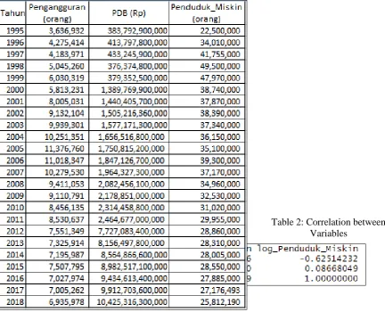
There are three variables that will be tested with regression. The variables are unemployment in Indonesia, poverty in Indonesia and constant GDP in Indonesia from 1995 to 2018. The unemployment and poverty data are obtained from Badan Pusat Statistik, while the constant GDP data is obtained from Bank Indonesia.

Relationship between variables are tested using R Studio with these functions

Regresi = lm(formula = Data$Y ~ Data$X1 + Data$X2, data = Data)

Regresi_transformasi = lm(formula = log(Data$Y) ~ log(Data$X1)+ log(Data$X2), data = Data)

where: Y = GDP

X1 = unemployment

X2 = poverty

4. RESULTS AND DISCUSSION 4.1. Impact of Unemployment on GDP

The estimated regression is:

Y = 3.832 x 1012- 24910 X1 (a)

where Y = GDP

X1 = unemployment

(6)

In regression a, it can be seen that the variables have different measurement so interpretations become more difficult. Thus log transformations are needed so that interpretations can be done in percentages.

The log regression is the following

Log Y = 3.7355 + 1.5581 Log X1 (b)

where Y = GDP

X1 = unemployment

After transformation, an increase in 1% in unemployment will increase GDP by 1.5581%. Unemplyoment is significant at 1%, and its variation explains 18.35% of GDP. Setelah transformasi regresi dilakukan, maka dapat dijelaskan bahwa setiap kenaikan 1% jumlah pengangguran akan menaikkan PDB sebesar 1,5581%. However, we only uses 24 data points, and 18.35% does not explain much.

GDP represents the sum of products and services in the economy. The GDP used in this analysis is GDP consant which shows that is is based on a certain year which makes the measurement more effective in showing the increase and decrease of productions.

Unemployment can be denoted as U = (1-N) / L where U = unemployed labour

N = employed labour L = total labour

In production functions, N ca be changed to GDP so that: U/L = 1-GDP

Thus, an increase in U will decrease GDP. This is shows in regression a although it is insignificant. In regression b, the impact of unemployment on GDP is not consistent with theory because it shows a positive relationship. Furthermore, the correlationb etween the variablesa re 0.428 which shows that they have a moderate correlation as it is between 0.4 and 0.599. Based on the discussion above, the impact of unemployment on GDP in Indonesia is not signficant as:

1. The significance is now compensated as it has low data points (n= 24 data).

2. Small R-squared valueJumlah pengangguran hanya dapat menggambarkan nilai PDB sebesar 18,35% (nilai R2 kecil)

3. It is economically insignificant.

4.2. Impact of Poverty on GDP

The estimated regression is the following: Y = 1.574 x 1013_{- 354700 X}

2 (c)

where Y = GDP X2 = poverty

An increase in poverty by 1 person will decrease GDP by 354700 rupiahs. It is significant as it can decrease up to 3.3 times of average GDP in Indonesia (1995-2018). It is statistically significant and its variation explains 43.54% of the variation in GDP.

In regression c, both variables have different measurements, so log transforamtions are done so that we can interpret in percentages.

Here is the estimated log regression:

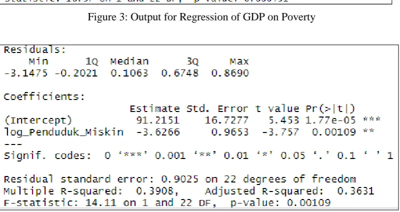
Log Y = 91.2151 – 3.6266 Log X2 (d)

(7)

An increase in poverty by 1% is expected to decrease GDP by 3.6266%. It is statistically significant, and its variation explains 39.08% of the variation in GDP. The correlation is 0.625, which means there is a strong inverse relationship as the magnitude is between 0.6 to 0.799.

Consumption is one of the factors that determines GDP. This can be seen from the equation Y = C + I + G + NX. The higher / lower the level of consumption of the Indonesian population, the higher / lower the value of GDP. To determine the level of consumption, a C [W, (Y - T)] function approach is used where:

W = Wealth (includes wealth in terms of financial, property, and income)

Y = Wages

T = Tax

When the number of poor people increases in Indonesia, the wealth factor will decrease so that the level of consumption also decreases. Declining consumption levels will then reduce GDP because the demand for goods and services produced by all economic units will decrease. Based on the explanation above, it can be stated that the effect of the number of poor people on GDP is in accordance with the theory that an increase in the number of poor people will reduce the value of GDP.

4.3. Impact of Unemployment and Poverty on GDP

The estimated regression is the following:

Y = 1,563 x 1013 + 15690 X1 - 354900 X2 (e)

where Y = GDP

X1 = unemployment

X2 = poverty

An increase in unemployment by 1 person is expected to increase GDP by 15690 rupiahs and an increase in poverty by 1 person is expected to decrease GDP by 354900 rupiahs. Based on the F-test, both variables jointly have a significant impact on GDP. 43.55% of the variation in GDP is explained by the variation in unemployment and poverty. Poverty is more dominant than unemployment because it is more statistically significant.

In regression e, we can see that the variables have different measurement so we transform them into log forms.

The log regression:

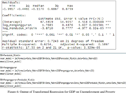
Y = 67.4819 + 1.7685 Log X1 – 3.8710 Log X2 (f)

dengan Y = GDP

X1 = unemployment

X2 = poverty

An increase in unemployment by 1% is expected to increase GDP by 1.7685% and an increase in poverty by 1% is expected to decrease GDP by 3.8710%. F-tests show that the variables are jointly significcant. 62.54% of the variation in GDP is explained by the variables. Poverty is more dominant that unemployment as it is more significant.

Regression f is chosen as:

1. 62.54% of the variation is explained. 2. Interpretations are easier.

(8)

4.4. Policy Implications

Based on the regression analysis, the government should focus on reducing poverty. This is because poverty has a significant impact on GDP and it lowering it by 1% can increase GDP by 3.8710%.

The factor that is related with GDP and poverty is consumption, as investment, government expenditure and net export are not to relevant. Consumption is directly related to a person's wealth, wage, and tax payments. To decrease poverty in Indonesia, wealth will be affected by how people compare their savings and their expenses. Taxed are based on PPh 21. For wages, it is based on:

Wage setting = Price Setting F (u,z ) = 1/(1+μ) where u = unemployment z = institutional factors μ = marked up price over cost

There are 2 factors that can be managed by government policies:

1. Wage structural regulations that can be used to manage wages so that institutions do not give late wages. This is used to manage wage settings. By regulating wages, institutions can increase employees' well-beging in terms of materials, poverty will decrease, public poewr of purchase will increase and GDP will increase.

2. Market monitoring regulations to make sure the market is competitive so that marked up price over cost is in a reasonable value. This is to regulate price settings to make competitive markets so that prices are not volatitle. Froma consumper's perspective, consumption on products and services will increase which will increase GDP. From producer's perspective, sales will increase which will increase real wages for employees so that poverty will decrease.

5. CONCLUSIONS AND RECOMMENDATIONS

Based on the regression analysis, here are the conclusions.

1. Unemployment has a signficant impact on GDP. An increase in unemployment by 1% is expected to increase GDP by 1.581%. 18.35% of the variation in GDP is explained by the variation in unemployment. Unemployment and GDP are positively correlated (0.428).

2. Poverty has a significant impact on GDP. An increase in poverty by 1% is expected to decrease GDP by 3.6266%. 39.08% of the variation in GDP is explained by the variation in poverty. Poverty and GDP are negatively correlated (-0.625).

3. Unemployment and poverty have a significant joint impact on GDP. An increase in unemployment by 1% is expected to increase GDP by 1.7685% and an increase in poverty is expected to decrease GDP by 3.8710%. 62.54% of the variation in GDP is explained by the variation in unemployment and poverty.

4. Poverty has a more dominant impact on GDP compared to unemployment.

5. The government should focus on reducing poverty to increase GDP. Consumption is the most significant indicator of GDP as it can affect wage and price settings.

Here is the recommendation:

(9)

REFERENCES

Blanchard, Olivier. (2000). Macroeconomics. New Jersey: Prentice-Hall, Inc.

BPS. (2019). Pengangguran Terbuka Menurut Pendidikan Tertinggi yang Ditamatkan 1986 -2018. diambil 29.11.2019 dari www.bps.go.id

BPS. (2019). Jumlah Penduduk Miskin, Persentase Penduduk Miskin, dan Garis Kemiskinan 1970 - 2017. diambil 29.11.2019 dari www.bps.go.id

BI. (2019). Produk Domestik Bruto Menurut Lapangan Usaha Atas Dasar Harga Konstan 2010. diambil 29.11.2019 dari www.bi.go.id

Mankiw, N. G. (2007). Makroekonomi (edisi ke-6). Jakarta: Erlangga.

Rstudio. (2019). diambil 29.11.2019 dari rstudio.com

Sugiyono. (2017). Metode Penelitian Kuantitatif, Kualitatif, dan R&D. Bandung: Alfabeta, CV.

Appendix List of Figures

(10)

Figure 2: Output for Transformed Regression of GDP on Unemployment

Figure 3: Output for Regression of GDP on Poverty

(11)

Figure 5: Output of Regression for GDP on Unemployment and Poverty

(12)

Figure 8. Transformed Regression Coding

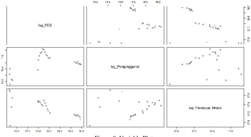
Figure 9. Variable Plots

(13)

Table 1: Data for Poverty, Unemployment and GDP for Indonesia from 1995 to 2018