Download Download PDF

164

Modelling Financial Contagion in the South African Equity Markets Following the Subprime Crisis *Olivier Niyitegeka, Dev D. Tewari

University of Zululand, South Africa [email protected]

Abstract: This paper used wavelet analysis and Dynamic Conditional Correlations model derived from the Multivariate Autoregressive Conditional Heteroskedasticity (MGARCH-DCC) to investigate the possible presence of financial contagion in the South African equity market in the wake of the subprime crisis that occurred in the United States. The study uses Dornbusch, Park and Claessens’s (2000) broader definition which asserts that financial contagion only takes place if cross-correlation between two markets is relatively low during the tranquil period, and that a crisis in one market results in a substantial increase cross-market correlation. Using wavelet analysis, the study found high levels of correlation during the subprime financial crisis in both smaller and longer timescales. In the former, high correlation was identified as financial contagion, whereas in the latter it was found to indicate co-movement due to financial fundamentals. The high correlation was identified for small scales 3, 4 and 5 that range from a week to one month indicates the presence of contagion. The study also used the MGARCH-DCC model to compare the cross-market correlation between the SA and the US markets, during a ‘pre-crisis’ and ‘crisis’ period. The study used data for the period between January 2005 and December 2007 for the ‘pre-crisis’ period and that for the period from January 2008 to December 2014 for the ‘crisis’ period. The results indicate cross-market linkages only during the crisis period; hence, it was concluded that cross-market correlation during the period of financial turmoil in the US was the result of financial contagion.

Keywords: Financial contagion, wavelet analysis, Maximal Overlap Discrete Wavelet Transform (MODWT),

MGARCH-DCC, subprime crisis.

1. Introduction

The 1990s will go down in history as a period of systemic financial crisis for emerging economies. The Latin American countries were the first to be hit following the 1994 Mexican peso crisis and its impact on other emerging markets (Kaminsky & Reinhart, 2000). This was followed by other crises that reverberated across emerging economies in Western Europe, East Asia and South Asia (Lam, 2002). Initially, much blame was directed toward poor domestic policies and little attention was given to the propagation aspect of these crises. It was only towards the middle of the 1990s, after more severe crises (such the Asian crises in 1994 and 1997, the Russian turmoil in 1998 and the Brazilian crunch in 1999) that researchers in the field of economics and finance started to document the propagation of these crises from one country to another (Kaminsky & Reinhart, 2000). These propagations are known as financial contagions. Kaminsky, Reinhart and Végh (2003) identified three key elements, which they dubbed the “unholy trinity”, that make emerging markets prone to contagions, they are: (1) a sudden reversal in the capital inflow in the economy, (2) an unexpected announcement, and (3) a leveraged common creditor. Regarding the reversal in capital inflow Kaminsky, Reinhart and Végh (2003) noted that it is due to the fact that, prior to financial contagions, crisis-prone markets experience a surge in international capital inflow.

165

The purpose of the study is twofold. First, it adds to the existing literature on financial contagions by testing lead/lag analysis between the US and SA equity markets, as well as testing whether or not the cross-market linkages between the US and SA equity vary over time and are asymmetric in tranquil periods compared to crisis periods. Secondly, the study provides information to investors and policymakers on the extent to which shocks in the US market affect the SA market. A better appreciation of correlations of returns in the two markets is crucial to efficient portfolio diversification. Furthermore, the understanding of cross-market correlation offers more insights to policymakers for potential decoupling or coupling strategies to protect the SA market from the contagious effects of the US market. A survey of the literature on contagion in the SA equity market by the authors identified two studies. The first, Collins and Biekpe (2003), investigated the contagion on African economies, including SA, in the wake of the Asian crisis in 1997. Using both the unadjusted and the adjusted correlation coefficient, they found evidence of financial contagion to the SA markets, only in the largest and most traded markets. The second study, Heymans and Da Camara, (2013) looked at cross-market linkages between SA and major stock market around the world, using an aggregate-shock model, they found evidence of volatility spill-over effects to the SA stock market originating from the Hang Seng, London, Paris, Frankfurt and New York stock markets.

The models used in the two studies above do not allow correlation between time series to be time-varying; furthermore, they do not allow conducting a lead/lag analysis between the time series. The current study sought to fill this gap by employing wavelet analysis and MGARCH-DCC model. Wavelet tools were appropriate because not only do they allow the conducting of a lead/lag analysis but they also enable the chronological specifications for financial variables to be examined, especially decomposing them into sub time series and by localising time series cross-correlation (Hashim & Masih, 2015). The MGARCH-DCC model was also employed as it allows correlations to be time-varying, in addition to the conditional variances. Hence, the researchers were able to assess whether or not, correlations between the US and SA stock markets are time-varying and evolve according to the situations that prevail in the markets (for example, periods of stability versus periods of turmoil). The remainder of the study is organised as follows. Section 2 presents a review of related work. Section 3 describes the models and the data employed, while Section 4 discusses the results. Conclusions and policy implications are presented in Section 5.

2. Literature Review

Despite the surge of interest in contagion, this concept has not been easy to define. Indeed, there have been disagreements on whether the term should apply between two countries that have similar macroeconomic fundamentals and are closely linked (Boyer, Dehove, & Plihon, 2004). For example, the US and Canada are located in the same geographic area and have many similarities in terms of market structure and history. These countries are always linked during stable and crisis periods. Therefore, propagation of a large scare during a period of crisis is simply a continuation of the interdependence that exists in stable periods. Forbes and Rigobon (2002) describe contagion as “a significant increase in cross-market linkage to one country or group of countries”. However, this is regarded as a narrow definition and is not unanimously approved. As Ranta (2010) maintains, financial contagion cannot only be described on the basis that changes in cross-market linkages have taken place. He argues that the investigation of contagion should focus on the spread of shock from one market to another.

166

However, their results indicated that for developed Pacific regions, certain sectors such as Technology, Healthcare and Consumer goods were less affected by the crisis; they also found that regions susceptible to be affected by contagious effects were observed in the emerging Asian and European regions. Ahmad, Sehgal and Bhanumurthy (2013) investigated finical contagion from Greece, Ireland, Portugal, Spain, Italy, USA, UK and Japan markets to BRIICKS (Brazil, Russia, Indonesia, India, China, South Korea and South Africa) bourses during the Euro-zone crisis period. Their empirical results indicated that among Eurozone countries, Italy, Ireland and Spain were most contagious for BRIICKS markets as opposed to Greece. The study also indicated that China, Brazil, India, South Africa and Russia, were greatly marked by the contagious effects during the Eurozone crisis. Nevertheless, they found that Indonesia and South Korea markets only experienced co-movement due to financial fundamentals and not contagion. Hemche, Jawadi, Maliki and Cheffou (2016) studied the contagion hypothesis, following the subprime crisis, for Argentina, China, Egypt, France, Italy, Mexico, Morocco, Tunisia and UK with regards to the US market. Their findings indicated that there was a rise in dynamic correlations for most markets hence the conclusion that financial contagion from the US market took place during the subprime crisis.

3. Data and Methodology

Data: This study aimed to investigate the financial contagion between the SA and US equity markets. The study used the daily stock return for the S&P 500 index as a proxy for the US stock market and the FTSE/JSE All Share index to represent the SA equity market. For wavelet analysis, the entire data from 2005 to 2015 was used. The use of a big sample for wavelet analysis was motivated by the fact that the model is able to dissect data into different scales, making it possible to decompose complex information and patterns into simple forms (Dajcman, 2013). For the MGARCH-DCC modelling the data was divided into two sets: (1) data for the ‘pre-crisis’ period between 01 January 2005 and 31 July 2007, and (2) data for the ‘crisis’ period from 01 August 2008 to 1 July December 2010. Splitting the data into two sub-periods (calm and turmoil periods) was done in order to allow the researchers to test whether or not volatility spill-over between SA and US stock markets varies from normal to turbulent periods1_{. The stock market indexes were transformed into}

logarithmic daily returns by taking the log difference of each index series, as follows:

 

 

1

ln

ln

t t t

R



P



P

_ ………..3.1

Where

R

_t is one-day return from the period t-1 to t,

P

_t is the daily closing price index recorded at t, and

P

_t1

is the daily closing price index recorded on the previous day t-1.

Wavelet Analysis: Wavelet analysis, according to Ranta (2010), offers researchers lenses where they can take a close-up look at the details and draw a holistic image of a series at the same time. The analysis entails estimating an initial series against a sequence of two elementary functions, called wavelets, these functions are, the father wavelet,

f

, and the mother wavelet, ψ. The mother wavelet can be enhanced and translated to form the foundation for the Hilbert space L2 ₍

¡

_{) of squared functions that can be integrated. The father and}

mother wavelets are formulated as follows:

 









2





,

2

2

j j j k

t

t k

………..3.2

 

2





,

2

2

j j j k

t

t

k











………..3.3

where j = 1, ..., J is the scaling parameter in a J-level decomposition, and k is a translation parameter (j,k

Î

¢

). The long-run trend of the series is depicted by the father wavelet, which integrates to 1. The mother wavelet, which integrates to 0, expresses fluctuations from the trend.

1 _{The authors are of the opinion that the period post December 2010 is characterised by another financial crisis}

167

The Maximal Overlap Discrete Wavelet Transform (MODWT) Wavelet Analysis: According to Abdullah, Saiti, and Masih,(2014), both the Discrete Wavelet Transform (DWT) and the Maximal Overlap Discrete Wavelet Transform (MODWT) possess the ability to decompose the sample variance of a time series. However, the MODWT relinquishes the orthogonal property of the DWT to acquire other characteristics. Hashim and Masih (2015 ) highlight the advantages of MODWT over DWT as follows: 1) the MODWT has the capability to handle any sample size irrespective whether or not the variables are dyadic; 2) it offers a bigger resolution at greater scales as the MODWT oversamples the data; 3) translation-invariance guarantees that MODWT wavelet coefficients do not alternate if the time series is modified in a ’circular’ fashion; and 4) the MODWT presents a more asymptotically effective wavelet variance than the DWT. The MODWT was chosen for the purpose of the current study.

The MODWT estimator of the wavelet correlation specified as follows:

 









   

Cov

,

Corr

,

Var

Var

ijt ijt

xy j ijt ijt

ijt ijt

 

 

 









………..3.4

where



_ijtrepresents the scale of wavelet coefficient



_j acquired by applying MODWT. The disintegration of the series using MODWT is achieved with Daubechies least asymmetric (LA) wavelet filter of length 8.

Wavelet Variance and Wavelet Correlation: The MODWT has the ability to break down a variance of a sample of a series on a scale-by-scale basis, due to the fact that MODWT conserves energy.

±

=

=

å

2

+

%

2

2

1

jo

j _jo

j

X

W

v

………..3.5

From equation 3.5 above a scale-dependent analysis of variance from the wavelet and scaling coefficients is Derived, as follows:

±

u

=

=

-

=

å

+

%

-%

_X2

X

2

X

2

1

_jjo₁

W

j 2

1

v

_jo 2

X

2

N

N

………..3.6

Percival and Walden (2006) highlight that wavelet variance is characterised for both stationary and non-stationary processes by letting {Xt : t = ..., –1, 0, 1, ... } be a discrete parameter real-valued stochastic process

whose d th-order differencing will give a stationary process

(

)

₌

æ ö÷

ç ÷

(

)

-º

-

º

_{ç ÷}

_{ç ÷}

-çè ø

å

0

1

d _t d_k

d

1

k _{t k}

Y

B X

X

k

………..3.7

With spectral density function (SDF) SY(.) and mean μY. Let SX (.) denote the SDF for {Xt}, for which SX (f) = S Y(f)/Dd(f), where D(f) ≡ 4sin2 (πf). Filtering {Xt} with a MODWT Daubechies wavelet filter

{ }

h

%

_{j l,} of width L ≤

2d, a stationary process of jth-level MODWT wavelet is derived as follows:

( )

-=

º

å

1

%

, _{, 1}

0

, t=...,-1,0,1...

Lj

j t _{j l t} l

W

h X

………..3.8

where

W

j t, is a stochastic process achieved by filtering {Xt} with the MODWT wavelet filter

{ }

h

%

_{j l,} and

(

)

(

)

º

2

j

-

1

-

1

+

1

j

L

L

.

With a series, which is the realisation of one segment (with values X0 , ..., XN – 1) of the process {Xt}. Under

condition Mj ≡ N – Lj + 1 > 0 and that either L > 2d or μx = 0 (realisation of either of these two conditions

implies

E W

_{

j t,

_}

=

0

and therefore

u

2_X

( )

τ

_j

=

E W

{

j t,

}

), an unbiased estimator of wavelet variance of scale

( )

(

u

2

)

j j

τ

_X

τ

is given by (Percival and Walden, 2006):

( )

±

u

-=

-=

å

)

₂ 1 2

,

j _{, 1}

1

τ

N j t

X _{t L}

j

W

M

168

where

_{

W

°

j t,

_}

are the jth-level MODWT wavelet coefficients for time series

±

( )

(

-

)

-=

º

å

1

%

, Lj_{0 , 1 modN}

, t=0,1...,N-1

j t _{l j l t}

W

h X

………..3.10

It can be shown that the asymptotic distribution of

u

)

_X2

_{( )}

τ

_j is Gaussian, which enables the preparation of confidence intervals for the estimate (Percival, 1995; Dajčman, 2013). Given two stationary processes {Xt}

and {Yt}, whose jth-level MODWT wavelet coefficients are

{

W

X j t, ,

}

and

{

W

Y j t, ,

}

an unbiased covariance

estimator

$

u

XY

_{( )}

τ

_j is specified by (Percival, 1995):

( )

±

( )

±

( )

{

}

u

-=

-=

å

=

$

1 _{, , , , , ,}

j

1

1

τ

N X Y

cov

,

XY j t j t X j t Y j t

t L

j j

W W

W

W

M

………3.11

With

M

_j

º

N L

-

_j

+ >

1 0

being the number of non-boundary coefficients at the jth-level. The MODWT correlation estimator for scale τj can be obtained by using the wavelet covariance and the square root of wavelet variances:

( )

( )

( ) ( )

u

r

u

u

=

)

)

)

)

, j , j j j

τ

τ

τ

τ

X Y X Y X Y ………..3.12

where

r

)

_{X Y,}

_{( )}

τ

_j

£

1

. The wavelet correlation is analogous to its Fourier equivalent, the complex coherency

(Gençay, Selçuk and Whitcher, 2003). Computation of confidence intervals is based on Percival and Walden (2006). With the random interval

( )

(

)

( )

(

)

r

r

-

-é

_ï

ì

_ï

_F

_-

ü

_ï

_ï

ì

_ï

_ï

_F

_-

_ï

_ï

ü

ù

ê

_ï

_é

_ù

_-

_ï

_ï

_é

_ù

₊

_ï

ú

í

ý

í

ý

ê

_ï

_ê

_ë

_ú

_û

_ï

_ï

_ê

_ë

_ú

_û

_ï

ú

ê

_ï

_ï

_î

-

_ï

_ï

_þ

_ï

_ï

_î

-

_ï

_ï

_þ

ú

ë

û

1 1

XY j XY j

j j

1 p

1 p

tanh h

τ

,tanh h

τ

N

3

N

3

………..3.13

Capturing the right wavelet correlation and providing an approximate of 100(1 – 2p)% confidence interval.

Wavelet Cross-Correlation: Cross-correlation according to Percival and Walden (2006), is a method in wavelet which entails computing the intensity of the correlation between to two series. The series can be shifted, (the series can lag if π is negative or they can lead when π is positive) and then the correlation between the two series is estimated. Cross-correlation analysis enables us to single out which series’ error terms are leading the other’s error terms, with the latter series considered as lagging. The size and magnitude of cross-correlation denotes whether the series that leads series has prognostic power over the series that lags. It is worth noting that, the wavelet cross-correlation also offers a lead/lag relationship on a scale-by-scale basis. The MODWT cross-correlation for scale-by-scale τj at lag π, is formulated as:

( )

( ) ( )

{

}

( )

{ }

( )

{

}

p p p

r

+ +

=

æ

_ö÷

ç

_÷

ç

÷

çè

ø

, ,

, j 1

2 , ,

cov

,

τ

var

var

X Y j t j t XY

X Y

j t j t

W

W

W

W

………..3.14

where ( ),

X j t

W

are the jth-level MODWT wavelet coefficients of series {Xt}, at time t, and ( ),

Y j t

W

+p are the

jth-level MODWT wavelet coefficients of series {Yt} lagged for π time units. Wavelet cross-correlation captures values,

- £

1

r

)

_p,XY

_{( )}

τ

_j

£

1

, for all τ and j.

169

( )

(

( )

)

( )

(

)

(

( )

)

--

-=

g

2 1

2

2 2

1 1

xy n n

x y

n n

S s W

s

R s

S s W s

S s W s

...3.15

where S is a smoothing operator, s is a wavelet scale, x

( )

n

W

s

is the continuous wavelet transform of the time

series X, y

( )

n

W

s

is the continuous wavelet transform of the time series Y, and xy

( )

n

W

s

is a cross-wavelet transform of the two-time series X and Y (Saiti, 2016). The supposition is that the lower scale high wavelet coherence is due to "contagion", and higher scale high coherence is due to "fundamentals" (Saiti, 2016).

MGARCH-Dynamic Conditional Correlation (DCC): The MGARCH-DCC model was formulated by Engle (2002) to capture the dynamic time-varying of conditional covariance. The MGARCH-DCC model is a dynamic model with time-varying mean, variance and covariance of return series

r

_t with the following equation:

t t t

r u

 



...……. 3.16





1

N 0,H

t t t



 

_

From the residuals of the mean equation, the conditional variance of each return is derived using equation (3.16) given below:

2 2 2

, 0 , ,

1 1

i i

p q

i t j i t j j i t j

j j

h



 

_

 

_

 











…………. 3.17

where .

Then the multivariate conditional variance

H

_tis estimated as follows:

t t t t

H



D R D

………….. 3.18

where

H

_tis the conditional covariance matrix of

r

_t,

D

_t represents a (k × k) diagonal matrix of time-varying standard deviations attained from the univariate GARCH specifications given in equation (3.17) ,

R

_tis the (k x k) time-varying correlations matrix derived by first standardising the residuals of the mean equation (3.15) of the univariate GARCH model with their conditional standard deviations derived from equation (3.17), to obtain



_it





_it

h

_it2.

The standardised residuals are then used to estimate the parameters of conditional correlation as given in equations (3.19) and (3.20) below:

 





1



 

1



2 2

t t

diag Q

diag Q

t t

R





Q

 …………. 3.19

and



1

1 2



1 1

'

1 2 1

t t t t

Q

  

 

Q



  

_{ }





Q

_ …………. 3.20

where

Q

is the unconditional covariance of the standardised residuals. The

Q

_t does not usually take ones

on the diagonal, so it is scaled as in equation (3.19) above, to derive

R

_t, which is a positive definite matrix. In this model the conditional correlations are thus dynamic, or time-varying.



₁and



₂from equation (3.20) are assumed to be positive scalars (



₁+



₂< 1).

1 1

1

 

 



pi



qi

j j

j j

170

The parameters of the MGARCH-DCC model are estimated using the likelihood for this estimator and can be written as:

 



1



1

1

_{log 2}

_2log

_log

_'

2

T

t t t t t

t

L

n



D

R



R







 









………3.21

where and

R

t is the time-varying correlation matrix.

4. Results and Discussion

Summary Statistics: The summary statistics of the data used in the study, namely, the log difference of daily stock return for the S&P500 index and for the FTSE/JSE All Share index, are listed in Table 1. These summary statistics are the sample mean, maximum, minimum, median, standard deviation, skewness, and Anderson-Darling normality test (with their p-value). From Table 1 it is evident that all the statistics are not normally distributed and have leptokurtic properties that are shared in most financial time series (Chinzara, 2006). For the two variables, the kurtosis is more than three, meaning that the distributions are slim and long-tailed (leptokurtic). This is confirmed by the Anderson-Darling normality test that shows a significantly low p-value in all the variables under consideration; hence, the rejection of the null hypothesis of a normal distribution.

Table 1: Summary Statistics of the Data

S&P 500 FTSE/JSE All Share

Number of observations 2867 2867

Mean 1.850610e-04 3.562482e-04

Median 7.822280e-04 7.215250e-04

Minimum -9.469514e-02 -7.580684e-02

Maximum 1.095720e-01 6.833971e-02

Standard deviation 1.404760e-02 1.305817e-02

Skewness -0.32 -0.13

Kurtosis 3.64 3.46

Anderson-Darling normality test 12.44 14.46

P value 2.2e-16 3.2e-18

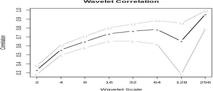
Results of the Wavelet Analysis: Figure 1 reports the wavelet (MODWT) estimator for wavelet correlation from the indices’ daily return series. The wavelet analysis was performed with eight scales that span from one day to one-and-a-half year dyadic steps (1-2 days, 2-4 days, 4-8 days, 8-16 days, 16-32 days, 32-64 days, 64-128 days and 64-128-256 days). Scales are presented on the horizontal axis and correlations on the vertical axis. To analyse statistical significance, 95% confidence intervals are used.

Figure 1: Wavelet Correlations between JSE/ALSI and S&P500

 

,



t i t

D

diag

h

*

*

*

* *

*

*

*

0.3

0.4

0.5

0.6

0.7

0.8

0.9

1.0

Wavelet Correlation

Wavelet Scale

Co

rre

lati

on

L

L

L

L L

L

L

L

U

U

U

U

U

U

U

U

171

It can be seen in Figure 1 that the wavelet correlations are all significantly positive. The correlation tends to increase as the scale increases. However, there is a sharp decrease on scale 7; thereafter the correlation increases again, reaching values close to unity at scale 8. This implies that discrepancies between the two equity markets do not dissipate for a period of less than a year. In other words, for the longer period, the correlation between the US and SA equity markets is more likely. This can also be construed as perfect integration between the US and SA equity markets. The study also examined cross-correlations between the JSE/ALSI and the S&P500 at all periods with the related estimated confidence interval against lead time and lags for the different wavelet scales up to 33 days. If the curve is substantially skewed on the right, the second variable, i.e. S&P500, is leading. Conversely, if the curve is considerably skewed on the left side of the graph, the first variable, i.e. JSE/ALSI, is leading.

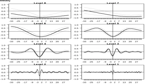
It can be seen in Figure 2 that the contemporaneous time scale correlation between the series indicates that the values of the wavelet correlation coefficients at lag 0 have an anti-correlation relationship. Figure 2 illustrates that at the shortest scales, i.e. scales 1 to 4, the cross-correlations around the time shift of π = 3 and

π = – 3 are significant and positive. It can also be seen that at these short scales the graphs are symmetrical

(zero skewness) meaning that there is no clear evidence of a lead-lag potential. For coarse scales, particularly scales 5 and 6, the highest correlation is achieved at time shift of π = 25 and π = – 25. It should also be noted that scales 5 and 6 the graphs are slightly skewed to the right indicating that S&P 500 leads the JSE/ALSI. This means that for a period two weeks to two months, the S&P 500 leads the JSE/ALSI for a period of 25 days. For scale 7 we can see that there is a significant negative wavelet cross-correlation on the right-hand side with implications that the S&P 500 leads the JSE/ALSI. As for scale 8 there is no clear evidence of a lead-lag relationship.

Figure 2: Cross-Correlation for Different Wavelet Scales with Leads and Lags Up to 33 Days (1.5 Months)

Figure 3 presents the estimated cross wavelet coherence between the S&P500 and the JSE/ALSI. The values for the 5% significance level presented by the curved line are achieved using the Monte Carlo simulations. The map presents the cross-coherency between the two series. The name of the variable displayed first is the first series (i.e. JSE/ALSI) while the following one is the second series (i.e. S&P500). In wavelet coherence mapping, time is displayed on the horizontal axis — which is converted to time units (daily)-whereas the vertical axis displays the frequency (the lower the frequency, the higher the scale). In Figure 3, warmer

Le ve l 8

Lag -1.0

-0.5 0.0 0.5 1.0

-33 -25 -17 -9 -3 2 7 13 20 27

Le ve l 7

Lag -1.0

-0.5 0.0 0.5 1.0

-33 -25 -17 -9 -3 2 7 13 20 27

Le ve l 6

Lag -1.0

-0.5 0.0 0.5 1.0

-33 -25 -17 -9 -3 2 7 13 20 27

Le ve l 5

Lag -1.0

-0.5 0.0 0.5 1.0

-33 -25 -17 -9 -3 2 7 13 20 27

Le ve l 4

Lag -1.0

-0.5 0.0 0.5 1.0

-33 -25 -17 -9 -3 2 7 13 20 27

Le ve l 3

Lag -1.0

-0.5 0.0 0.5 1.0

-33 -25 -17 -9 -3 2 7 13 20 27

Le ve l 2

-1.0 -0.5 0.0 0.5 1.0

-33 -25 -17 -9 -3 2 7 13 20 27

Le ve l 1

-1.0 -0.5 0.0 0.5 1.0

172

colours (red) signify regions with major interrelation, while colder colours (blue) signify minor dependence between the series. Cold regions outside the significant areas represent time and frequencies with interdependence in the series.

Figure 3: Wavelet Coherence Mapping for the JSE/ALSI versus the S&P500

Arrows in the wavelet coherence plots represent the lead/lag phase relations between the observed series. Arrows point to the right indicate that the time series are moving in the same direction (in phase), whilst arrows pointing to the left indicate that the series move in opposite direction (anti-phase). Arrows directing South-East (right-down) or North-West (left-up), indicate that the first variable is leading, while arrows indicating to the North-East (right-up) or South-West (left-down) show that the second variable is leading. Figure 4 displays the direction of the arrows and their meaning.

173

It can be seen from Figure 3 that the direction of the arrows at different frequency bands differs over the study period. The ‘crisis’ period (between January 2008 and December 2010), is characterised by warmer colours, indicating high correlation during this period. It is also worth drawing to the reader’s attention that during periods of high correlation, the arrows mainly point North-East, indicating a positive correlation with S&P500 leading. For instance, for scales 3, 4 and 5 corresponding to a period from one week to one month, there is a high correlation for the period between 2008 and the beginning of 2011, which is the ‘crisis’ period. As Saiti (2016) explains, the high correlation in lower scales indicates the presence of contagion. It can also be seen in Figure 3 that for a very short scale of 1 and 2, i.e., the ones consisting of 2-4 days and 4-8 days, there is a low correlation between the JSE/ALSI and S&P500 along the observation period. For long-term investors (256-512 days holding periods), there are strong correlations between the S&P500 and the JSE/ALSI from 2007 to 2011. It is also worth noting that during this period the direction of the arrows indicates a positive correlation, with the S&P500 leading the JSE/ALSI. These results confirm those obtained in Figure 2 which indicates that longer high correlation is found in longer holding periods and this is indicative of co-movement due to fundamentals.

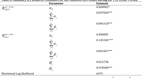
Estimations of the MGARCH-DCC Model: Summary estimates of the MGARCH-DCC model parameters are displayed in Table 2 for the ‘pre-crisis’ period.

Table 2: Summary of Parameter Estimates for the MGARCH-DCC Model during the ‘Pre-Crisis’ Period

Parameter Estimate

& ,

pre crisis S P t

R





0 0.000002*

1

i p

j j







0.097050***

1

i q

j j







0.896318***

,

pre crisis alsi t

R





0 0.000005

1

i p

j j







0.145248 ***

1

i q

j j







0.845467***

1



0.012738

2



0.978908***

Maximised Log likelihood 6475

It can be seen in Table 2 that the univariate GARCH (1,1) parameter estimates

1

i p

j j





and

1

i q

j j





are

statistically significant. Furthermore, the volatility persistence

1 1

i i

p q

j j

j j





 







is significantly close to unity, indicating strong volatility persistence between the SA and US markets for the “pre-crisis” period. The MGARCH-DCC correlation parameters are different from zero, implying that the correlations between the US and SA markets were dynamic during the pre-crisis period. Furthermore, the correlation parameter estimates show adherence to the restriction imposed on them, that is, of 𝜃1 + 𝜃2 = 0.9916 < 1, suggesting that the

estimated correlation matrix Rt is positive definite. However, the parameter estimate 𝜃1 is not statistically

174

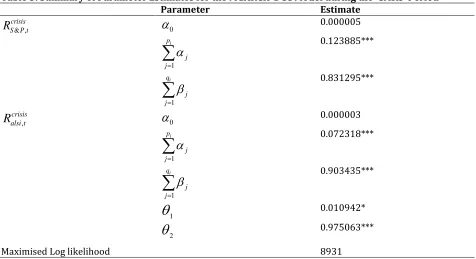
Table 3: Summary of Parameter Estimates for the MGARCH-DCC Model during the ‘Crisis’ Period

Parameter Estimate

& ,

crisis S P t

R



0 0.000005

1

i p

j j







0.123885***

1

i q

j j







0.831295***

,

crisis alsi t

R



0 0.000003

1

i p

j j







0.072318***

1

i q

j j







0.903435***

1



0.010942*

2



0.975063***

Maximised Log likelihood 8931

***Significant at 1%, ** Significant at 5%, * Significant at 10 %

Table 3 presents parameter estimates for the MGARCH-DCC for the crisis period. These results are similar to

the pre-crisis period in that the univariate GARCH (1,1) parameter estimates i p

j j=1

α



and

1 i

q j j







are

statistically significant. Furthermore, the volatility persistence measured by

1 1

i i

p q

j j

j j





 







provides

evidence of strong volatility persistence between the US and SA markets for the crisis period, as the estimated

coefficients

1 1

i i

p q

j j

j j





 







are significant and close to unity.

In addition, the correlation parameter estimates show adherence to the restriction imposed on them, that is, of 𝜃1 + 𝜃2 = 0.986005< 1, suggesting that the estimated correlation matrix Rt is positive definite. The fact

that the parameter estimates are statistically significant implies that the correlation is dynamic. Given the fact that the dynamic correlation is only significant during the ‘crisis’ period and is not significant in the ‘pre-crisis’ period, implies that co-movement between the US and SA markets during the ‘‘pre-crisis’ period was due to financial contagion, as a significant increase in cross-market linkages was only identified in that period. The above results are in line with the results from the wavelets analysis where high correlation was identified during periods of financial turmoil.

5. Conclusion

175

identified for shorter scales (3, 4 and 5) that range from two weeks to one month, which is indicative, the presence of contagion. The study also used the MGARCH-DCC model to compare the cross-market correlation between the SA and the US markets, during a ‘pre-crisis’ and ‘crisis’ period. The study used data for the period between January 2000 and December 2007 for the ‘pre-crisis’ period and that for the period from 01 August 2008 to 1 July December 2010 for the ‘crisis’ period.

The results indicate market linkages only during the ‘crisis’ period; hence, it was concluded that cross-market correlation during the period of financial turmoil in the US was the result of financial contagion. The results are in line with Maliki and Cheffou (2016) who identified financial contagion in emerging markets following the subprime crisis. The results also confirm Heymans and Da Camara’s (2013) findings. Form the above results the study suggests the following recommendation. Since the volatility spill-over between the US and SA market is unidirectional, with the US market leading the SA market, the implications thereof are that policymakers should focus more on monitoring the volatility of the US stock market, as effort by the South African authorities to stabilise volatility spill-over from the US market to SA market will be futile. Regulatory authorities should come up with sound risk management policies and macro-prudential regulations that enable investors to reduce significantly volatility exposure from the US market.

References

Ahmad, W., Sehgal, S. & Bhanumurthy, N. R. (2013). Eurozone crisis and BRIICKS stock markets: Contagion or market interdependence? Economic Modelling, 33, 209-225.

Boyer, R., Dehove, M. & Plihon, D. (2004). Les crises financières. Paris: La Documentation Francaise.

Chinzara, Z. & Aziakpon, M. J. (2009). Dynamic Returns Linkages and Volatility Transmission between South African and World Major Stock Markets. Studies in Economics and Econometrics, 33(3), 69-94.

Collins, D. & Biekpe, N. (2003). Contagion and interdependence in African stock markets. South African

Journal of Economics, 7(1), 181-194.

Dajcman, S. (2013). Interdependence between some major European stock markets—a wavelet lead/lag analysis. Prague economic papers, (1), 28-49.

Dornbusch, R., Park, c. y. & Claessens, S. (2000). Contagion: Understanding How It Spreads. The World Bank

Research Observer, 15(2), 177-197.

Engle, R. (2002). Dynamic conditional correlation: A simple class of multivariate generalized autoregressive conditional heteroskedasticity models. Journal of Business & Economic Statistics, 20(3), 339-350. Forbes, K. J. & Rigobon, R. (2002). No contagion, only interdependence: measuring stock market

co-movements. The Journal of Finance, 57(5), 2223-2261.

Gençay, R., Selçuk, F. & Whitche, B. (2003). Systematic risk and timescales. Quantitative Finance, 3(2), 108-116.

Hashim, K. K. & Masih, M. (2015). Stock market volatility and exchange rates: MGARCH-DCC and wavelet

approaches.". Retrieved 03 18, 2018, from

https://mpra.ub.uni-muenchen.de/65234/1/MPRA_paper_65234.pdf

Hemche, O., Jawadi, F., Maliki, S. B. & Cheffou, A. I. (2016). On the study of contagion in the context of the subprime crisis: A dynamic conditional correlation–multivariate GARCH approach. Economic

Modelling, 52, 292-299.

Heymans, A. & Da Camara, R. (2013). Measuring spill-over effects of foreign markets on the JSE before, during and after international financial crises. South African Journal of Economic and Management Sciences, 16(4), 418-434.

Kaminsky, L. G. & Reinhart , M. C. (2000). On crises, contagion, and confusion. Journal of International

Economics, 51(1), 145-168.

Kaminsky, G. L., Reinhart, C. M. & Vegh, C. A. (2003). The unholy trinity of financial contagion. Journal of

economic perspectives, 17(4), 51-74.

Kenourgios, D. & Dimitriou, D. (2015). Contagion of the Global Financial Crisis and the real economy: A regional analysis. Economic Modelling, 44, 283-293.

Lam, E. (2018). Dollar Index replaces VIX as new market gauge of fear. Retrieved March 03, 2018 from https://www.bloomberg.com/news/articles/2018-05-17/dollar-index-replaces-vixnewmarket-gauge-of-fear-chart

176

Office of the United States trade representative (2018). Retrieved June 11, 2018

Percival, D. B. & Walde, A. T. (2006). Wavelet methods for time series analysis (Vol. 4). Cambridge university press.

Percival, D. P. (1995). On estimation of the wavelet variance. Biometrika, 83(2), 619-631.

Ranta, M. (2010). Wavelet multiresolution analysis of financial time series. Helsinki: Universitas Wasaensis. Saiti, B. (2016). Testing the Contagion between Conventional and shari'ah-Compliant Stock Indices: Evidence

from Wavelet Analysis. Emerging market Finance and trade, 52(8).