The Socio Economic Determinants of Income Inequality in Pakistan
Adiqa Kiani
1Sara Siddique
2, Saima Sheikh
3Abstract
This study aims to examine the socio economic determinants of income inequality in Pakistan. For this analysis, data was taken from Pakistan Social and Living Standards Measurement (PSLM) 2013-14. Squared Coefficient of Variation (SCV) is used as dependent variable to measures income inequality. OLS regression model was used and the results show that individual level variable, i.e. gender, age and education level have positive impact on income inequality while age-square, marital status and occupation have negative impact on income inequality in Pakistan. The impact of family size and dependency ratio on income inequality in significantly positive indicating that increase in family size and non-working individuals in household induce income inequality. Income received through transfer payments or remittances reduce income inequality. It is recommended that in improving the quality of education and by reducing the gap of education vs uneducated, income inequality may decline. Different support programs and transfer payments to the poor further reduce the gap of rich and poor.
Keywords: Dependency Ratio, Remittances, Transfer Payments Introduction
Growth is not only the indicator that is sufficient for improvement in the standard of living of people but many other indicators involve in it[Alkire, S(2013)] Growth accompanied by unequal distribution of wealth/income might reduce the standard of the living of the people further and induced poverty [Alkire, S(2013)] . Unequal distribution of income directly impact poverty as it is a direct measure that shows how the benefit of economic growth is distributed among the society and indirectly affects poverty as it reduced the economic growth itself OECD Report (2016). Therefore, in those economies where the income gap between rich and poor is high and the income distribution is unequal among individuals, the economic development would be negative and poverty might be high.
1
Associate professor, Federal Urdu University Islamabad. 2
Mphil Economics, Federal Urdu University Islamabad, 3
Like many developing countries Pakistan is experiencing the stated issues which causing to the major economic problem, the income inequality. Despite the reasonable economic growth that Pakistan has achieved since its independence in 1947, poverty remains widespread, which is often attributed to the unequal distribution of income[World Bank Report(2016) Empirically the study measured poverty via Gini coefficient. The value of Gini coefficient decreased from 0.366 to 0.339 during 1964-1971. But after that income
inequality increased during 1970’s and Gini coefficient reached to 0.394 in
1979, which further increased during 2002, and reached to 0.419 which indicates that the gap between rich and poor has been increase in Pakistan from the last few decades Kemal, A.R. (2003)
The study main concern is to identify the factors which widen the gap between rich and poor. Various studies have examined the impact of macro and micro level socio-economic and demographic determinants of income inequality. Some studies have shown that individual characteristics including age, gender and education level are the most important determinants of income inequality. People with high education level have higher income level. Non-farm income, transfer payments, remittances and wage are also contributed to inequality in income among individuals.
In Pakistan, the issue of income inequality and its determinants has been discussed by many researchers. They have discussed the issue of inequality in income level, income gap, consumption and educational inequality and analyzed significant individual and household level determinants of income inequality. But there are some issues with the previous literature. Most of studies based on time series data computed inequality in income. Other studies have only discussed the issue of expenditure and educational inequality. Previous studies have conducted the household level analysis for income inequality. There is some critical variables/factor such as individual age, gender and education level etc. that have significant role in explaining the income inequality but those variables have been ignored. Another issue is that these studies based on small sample size and focused rural region Further focus of these studies was on aggregate level analyses for overall Pakistan.
inequality in which for the first time in Pakistan. For the purpose this study used Squared Coefficient of Variation (SCV) for the measurement of income inequality in Pakistan. For this analysis most recent available dataset of PSLM 2013-2014 was utilized.
Literature Review
There are various studies available examined the issue of income inequality[Mention in study]some are individual level, household level and regional level. Social characteristics mentioned in literature that few of them are showing significant role in determining income level and gap in income level among individuals. In this section, a brief review of the past literature on income inequality and its determinant has been presented.
De Kruijik and Naseem examined income inequality in Pakistan for the period 1970 to 1979. Gini coefficient, Theil index and coefficient of variation are used for analyses. Their findings showed that during the period of analyses the inequality has increased in Pakistan. Further their findings suggested that income inequality is more in urban than rural sample. Jafri et al compared regional wise inequality between urban and rural for the period 1979 to 1991 by using Gini coefficient in their study. They concluded that during 1988 the inequality has improved but increased substantially during 1991. Further they concluded that inequality was higher for urban sample than rural.
Numerous literatures are available which examined the determinants of inequality in income in Pakistan. Adam and He examined the sources of income inequality and poverty in rural Pakistan during 1986/7-1988/9. They decomposed the sources of income inequality in five major components. The results found that non-farm income and live-stock reduced income inequality while income from agriculture, rental and transfer payment enhanced overall income inequality. The finding of this study is analogous to the findings of Adam (1994).
Deininger and squire proposed new data set on unequal distribution of income. In their study they presented the criteria for selecting data on different groups of individual quintile and Gini coefficient. The quality of new data set is improved and covering large sample. Results based on new dataset show that there is no significant relation between growth and changes in overall inequality but there exist a significant positive association between growth and poverty alleviation.
and wage contributed more to income inequality. The results also suggested
that developing of aquaculture in 1980’s was main stimulated of inequality in
income.
Gregorio and Lee (2002) empirically examined the relation between education and income distribution by using panel data of more than 100 countries during 1960 and 1990. From the analyses they suggested that higher education and equal distribution of education have a significant impact on equal distribution of income among individuals. The relation between income and income inequality is inverted-U shape Kuznets curve. Further they recommended that government transfer payment expenditures have a significant role in making equal distribution of income. Field (2003) proposed new methods to decompose income inequality and changes in inequality over time in United States during 1979 and 1999. Empirical results based on new methods show that schooling is the main factor that explained inequality in income followed by occupation of individual.
Ssewanyana et al. (2004) explored the determinants of inequality in Uganda. In their study, they focused on sources of income and expenditure inequality and micro level factors that contributed to inequality. The results suggests that individuals of higher income groups having more productive assets are most likely to get extra benefit from national income, and richer became richer over time. Education is an important determinant of difference in income. Further they suggested that non-firm income is distributed unequally among people and mostly benefiting rich people. They also concluded that inequality within region is higher than among regions.
Idrees (2006) analyzed income and consumption inequalities and their various dimensions by employing various approaches of inequality. For the analyses he used micro panel data of HIES. The results indicated that general inequality in income and consumption is greater than adult per equivalent inequality. Regional wise analysis revealed that inequality is more in urban than rural. Decomposition level analyses shows that non-earned income contributed more to income inequality and non-food consumption is a major component of consumption inequality. Further he concludes that earning inequality is higher among female, younger and low educated individuals.
location of household affects both level of income inequality and changes in income inequality over time.
Aikaeli (2010) investigated the socioeconomic and geographic factors that affect income level of the households in rural Tanzania. For the analyses he used Generalized Least Square (GLS). The study concluded that household head education, number of working members of household, land ownership and non-farm enterprise positively impact income of the rural households. Households with female head reported lower income than male headed households. Further the study found that climatic variables i.e. rain fall have a positive impact while floods negatively affect the rural income.
Farooq (2010) analyzed the impact of education inequality both in urban and rural areas on gender base by applying Gini-Coefficient model using data from PSLM Survey of 2004-05. His results favored gender inequality in income distribution and he further noted that inequality among male workers was higher as compared to their female counterparts. He also found greater income inequality in urban areas as compared to rural areas with a favorable effect of education on income distribution.
Aikaeli (2010) studied different variables of income inequality using data from Rural Investment Climate Survey of Tanzania (2005) with estimation of linear models by applying a generalized least squares technique and found that incomes of households in rural areas is significantly and positively affected by improvements in variables like household labor force
size, household head’s education level, non-farm ownership of rural enterprise and land use in acreage. The results showed that income in
household’s having male as their head was significantly higher than in
households where female was the head and also having a positive effect of greater use of telecommunications and improvements in road infrastructure on rural incomes at the community level.
disparity across country are the dominant factors that have a significant impact on income inequality. Further they concluded that these factors affect poor and rich differently.
Data and Methodology
Data: To analyze the socio-economic determinants of income inequality in Pakistan, we have used data taken from Pakistan Social and Living Standards Measurement 2013-14.
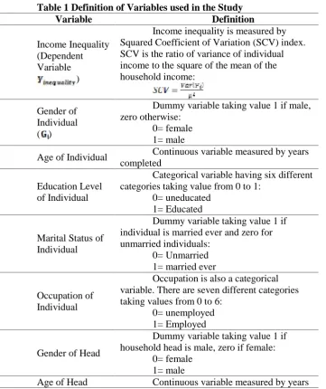
Table 1 Definition of Variables used in the Study
Variable Definition
Income Inequality (Dependent Variable
)
Income inequality is measured by Squared Coefficient of Variation (SCV) index. SCV is the ratio of variance of individual income to the square of the mean of the household income:
Gender of Individual ( )
Dummy variable taking value 1 if male, zero otherwise:
0= female 1= male
Age of Individual Continuous variable measured by years completed
Education Level of Individual
Categorical variable having six different categories taking value from 0 to 1:
0= uneducated 1= Educated
Marital Status of Individual
Dummy variable taking value 1 if individual is married ever and zero for unmarried individuals:
0= Unmarried 1= married ever
Occupation of Individual
Occupation is also a categorical variable. There are seven different categories taking values from 0 to 6:
0= unemployed 1= Employed
Gender of Head
Dummy variable taking value 1 if household head is male, zero if female:
0= female 1= male
completed
Education Level of Head
Categorical variable having five different categories taking value from 0 to 1:
0= uneducated 1= Educated
Marital Status of Head
Dummy variable taking value 1 if household head is married ever and zero if unmarried:
0= unmarried 1= married ever
Family Size Total member of the household. Continues variable
Dependency Ratio
Ratio of the member of the household of aged 0-14 years & above 64 years to the
members of the household of aged 15-64. Individuals of aged (0-14 & above 64)/individuals of aged (15-64).
Region
Dummy variable taking value 1 if household belongs to urban region and taking value zero if household located in rural region.
0= Rural 1= Urban
Total Income
Total income received by the members of household during one year (continue
variable) taken as independent variable.
Figure1: Region wise Distribution of Households (Percentage).
Now in province wise distribution, Baluchistan consist 9% of households, Khyber Pakhtunkhwa consist 20% of households, Punjab consist 42% of households and Sind consists29% of households. The distribution of PSUs and Households across region and province are given in figure-3.2.
Figure 2: Province Wise Distribution of Households (Percentage)
Source: Author’s Calculation
Methodology
Determinants of Income Inequality
In order to analyze the determinants of income inequality in Pakistan the following model4is utilized. (Adams and He, 1995; Aikaeli, 2010)
The general form of the model is given as:
(1)
In equation 1, is dependent variable, is the vector of
explanatory variables and is the error term that comprises the impact of all excluded variables.
The specific form of the model is given as:
(2)
In equation 2, is the measure of individual income
inequality, is the vector of individual characteristics, include age,
square, marital status, education level and occupation of the individual. is the vector of household level variables including age, gender and education level of the household head, family size, dependency ratio, transfer payments etc.(For detail see section 3.3 explanation of variables in below).
In order to see regional disparities in income a dummy for region is included.
(3)
is the regional dummy variables, showing =1 for urban and =0 for rural.
In order to see gender wise differences in income we alsoinclude a dummy for gender.
(4)
is the gender dummy variables, showing =1 for male and =0 for female.
We have estimated equations (5) for our analysis to measure income inequality.
The extended form of the model is given as:
(5)
SCV Calculation
Let there are member of household and is the average income of
(A)
Here is the variance of the income received by individual i
and is the square of the household’s average income.
Average of income and Variance of income can be calculated as;
Now putting the value of in equation (A)
(B)
The SCV is index of values whichvaries acrossindividuals. From equation (B) the SCV index is used as a proxy for income inequality ( ) in regression equations (5).
To calculate the variable SCV from the survey data we have to follow the following steps.
Equation “a” is called the average individual income.
We also calculated the square of average household income (
In the next step we subtract individual income from their respective household average income
Then take square of that
This term was aggregated at household level
Then divide the above term by family size
Equation “c” is called the variance of the individual income
Results and Discussions
Summary Statistics of Variables (Individual Level)
In this section we have presented the summary statistics of some important variables in table 4.1. For individual level of characteristics, the total numbers of observations are 81512. Gender of individuals have mean 0.49 which shows that on the average 49 percent of individuals are males whereas the remaining 51 percent are females and the standard deviation is 0.5 which represents variations in the values from their mean value. As gender of individual is dummy variable (taking value 1 if male, zero otherwise) for this study, the minimum value that is 0 which represents the female while the maximum value is 1 which represents male. Age of individuals have mean of 28.88 which shows that the mean age of individual is about 29 year and the standard deviation is 14.917.The minimum age of individuals is 10 years whereas the maximum age of individuals is taken as 65 years. Income of individuals have mean of Rs. 54435.51 which shows that the mean income of individual is about Rs. 54000. The range of income of individual is from Rs. 0(minimum) to Rs. 51000000 (maximum).Education of individuals have mean of 0.58 which shows that 58 percent of individual has attained the level of education whereas 42 percent of individuals are uneducated and the standard deviation is 0.494 which represents variation in the values from their mean value. The minimum education of individuals is 0 (no schooling) whereas the maximum education of individuals is 1 which mean that individual is educated. Marital status of individuals is a dummy variable having mean of 0.55 which shows that about 55 percent of individuals are married and 45 percent of individual are unmarried whereas variation in the value is0.498 (standard deviation). The minimum is 0 which shows that the individual is unmarried whereas the maximum value is 1 show that the individual is married. Occupations of individuals have mean/average of 2.00 and the standard deviation is 2.558. The occupation of individual is a categorical variable so the minimum is 0 which mean the individual have no job while the maximum is of individuals is 1 which represent that individual have job.
Table 2 Summary Statistics of Variables (Individual Level aged 10 to 65)
Variable Obs Mean Standard
Deviation Min Max
Gender 81512 0.49 0.500 0 1
Age of Ind. 81512 28.88 14.917 10 65
Education level. 81512 0.58 0.494 0 1
Marital Status 81512 0.55 0.498 0 1
Occupation 81512 0.42 0.493 0 1
Source: Author’s Calculation based on PSLM 2013-14
Summary Statistics of Variables (Household Level)
Now for household level of characteristics, the summary statistics of variables are in table 4.2, whereas the total number of observationsis17988.Gender of household head having mean 0.90 which shows that on the average 90 percent of household heads are males whereas the remaining 10 percent of the households are headed by females. The standard deviation is 0.295 which represents variations in the observations from their mean value. As gender of household is dummy variables for this study, the minimum value that is 0 which present female heads while the maximum value is 1 which is for male heads. Age of household head have mean 45.39 which shows that the average age of household head is about 45 year and the standard deviation is 13.686. The minimum age of household head is 15 years whereas the maximum age of individuals is taken as 99 years. Education level of household head having mean/average of 0.545 and the value of standard deviation is 0.4979. The minimum education of household head is 0 which show that the individual is not educated whereas the maximum education of household head is 1 which shows that the individual is educated. Marital status of household head have mean value of 0.98 which shows that about 98 percent of household heads are married and 02 percent of individual are unmarried and the standard deviation is 0.143. The minimum 0 shows that the head is unmarried whereas the maximum 1 shows that the household head is married. Family size of household head having mean/average of 6.64 which shows that family consist of approximately 7 members. The minimum 1 show that the family size consist of only 1 member whereas the maximum 47 shows that the family size consist of 47 members. Income of household head having mean/average of Rs. 18400 and the standard deviation is 516624. The minimum 0 shows that the household have zero income whereas the maximum Rs. 5133600 shows the highest income. Region is a dummy variable taking a value of 1 for urban region and 0 for rural region. The mean value of region is 0.35 which means that on average 35 percent of the household are living in urban areas whereas 65 percent of household are living in rural areas. The minimum 0 shows that the household living in rural area whereas the maximum 1 shows that the household living in urban area.
household have no income received through transfer payments or through remittances while maximum 1 shows the amount of transfer payments and/or remittances received by any household.
Table 3 Summary Statistics of Variables (Household Level)
Variable Obs Mean SD Min Max
Gender of Head 17988 0.90 0.295 0 1
Age of Head 17988 45.39 13.686 15 99
Education level of Head 17988 0.545 0.4979 0 1
Marital Status of Head 17988 0.98 0.143 0 1
Family Size 17988 6.64 3.253 1 47
Income of Household 17988 184000 516624 0 51336000 Transfer Payments &
Remittances 17988 0.43 0.495 0 1
Region 17988 0.35 0.476 0 1
Source: Author’s Calculation based on PSLM 2013-14
Overall Sample
The results for the overall sample are given in table 4. The coefficient of individual gender is 0.039 and significant at 1 percent. It means that income inequality is more among male than female. The coefficient of individual age variable is significantly positive (0.024) which means that with increase in age the income inequality increases but the age-square coefficient is negative means that after some point if age increase the income inequality will decreases. The impact of marital status of individual on income inequality is negative means that income inequality is lower if individual is married. The relationship of education of individual and income inequality is positive means that education increases the income inequality. The justification for the positive relation is that we have used education is categorical variable and the income of uneducated will be less than income of educated individuals. The coefficient of occupation of individual has significantly inverse relation with income inequality. If people have good occupation than they will get higher income and the inequality in income among people will decrease and vice versa.
Table 4: Regression Results of Overall Sample
Individual Level Variables Household Head’s Variables
Variable Coefficie nt
Std. Error
P-Value Variable
Coeffici
ent Std. Error P-Value
Constant -1.018 0.092 0.000
Gender_ind 0.039 0.020 0.054 Gender_head 1.569 0.034 0.000
Age_ind 0.024 0.003 0.000 Age_head -0.019 0.0007 0.000
Age2_ind -0.0001 0.0000
4 0.007
M.status_ind -0.452 0.030 0.000 M.status_hea
d 0.947 0.065 0.000
Edu_ind 0.0215 0.021 0.000 Edu_head 0.242 0.019 0.000
Occup_ind -0.560 0.021 0.000
Other Variables
Size_family 0.354 0.002 0.000
Dep_Ratio 0.621 0.011 0.000
Transfer_Pay
ments -0.086 0.017 0.000
Region -0.299 0.018 0.000
R-Square 0.3315
Sample Size 81512
* Standard errors are clustered at village level: Dependent Variable is SCV.
positive while age of the head coefficient is significantly negative. The education level and marital status of the household head have positive relationship with income inequality. It means that in those households where head are educated, the income level will be higher than those households having uneducated head which induce income inequality.
by individual will decrease. Similarly, if there are more dependent members in the household, the income of the earner in the household will be distributed among more individuals. Hence the income level of those individuals belong to large family size will be less than those individuals who belong to small family size and the income inequality increases in the overall society. The coefficient of transfer payments is negative and significant. Which shows that income inequality reduces when individual get transfer payments and remittances.
Table 5: Regression Results of Gender Wise Separate Analyses of Urban Sample
Individual Level Variables Household Head’s Variables
Variable
Male Female
Vari able
Male Female
Coeft. Std.Erro r
P-Va lu e
Coeft. Std.Error P-Val ue Co eft. Std. Erro r P-V al u e Coeft. Std . Err or P-Valu e
Constant -0.830 0.207 0.00 0 -0.526
0.20 2 0.009
Gen der_ Hea d
1.1 83 0.081
0. 0 0 0
1.305 0.066 0.000
Age_ind 0.038 0.00 8
0. 00
0 0.040
0.00 8 0.000
Age _ hea d -0.0 16 0.00 1 0. 0 0 0
-0.020 0.001 0.000
Age2_in
d -0.003 0.001
0. 00
2 -0.0003 0.00 1 0.000
M.status _ ind -0.054 0.07 0 0. 44 4 -0.826 0.06 6 0.000
M.st atus _ Hea d 1.0 83 0.132
0. 0 0 0
1.085 0.139 0.000
Edu_ind 0.369 0.061 0.00
0 0.107
0.04 7 0.022
Edu _hea d
0.1 32 0.049
0. 0 0 7
0.230 0.043 0.000
Occup_
ind -0.979 0.052 0. 00 0 -1.150
0.06 1 0.000 Other Variables
Size_
family 0.271 0.005 0.000 0.292 0.005 0.000 Dep_Ratio 0.807 0.030 0.000 0.559 0.027 0.000
Transfer_ Payments -0.04 8 0.03
7 0.199 -0.084 0.038 0.028
R-Square 0.2844 0.2849
Size 76
Gender Wise Separate Analyses of Both Regions (Urban)
We conduct gender wise separate analyses in both regions in order to see the gender wise difference of socio economic determinants of income inequality in urban and rural. The results are given in table 5. In urban age of both gender have significantly positive effect on income inequality. Age square have significantly negative effect on income inequality. The marital status has negative effect on income inequality but significant only for female. The impact of education is positive and significant on for female in urban. The impact of individual occupation on income inequality is negative and significant for both genders in urban regions.
Gender of the household head and head’s marital status has shown
significantly positive impact on income inequality for urban while age of the head has shown negative relationship with income inequality for both genders in urban. The coefficient of head education level is positive and significant for both genders in urban region.
The impact of family size and dependency ration on income inequality is significant and positive for both samples in urban. It means that increase in family size and increase in non-working (dependent) members of the household increase income inequality. Transfer payments negatively affect income inequality of both genders but only significant for female in urban region.
Gender Wise Separate Analyses of Both Regions (Rural)
Table 6: Regression Results of Gender Wise Separate Analyses of Rural Sample
Individual Level Variables Household Head’s Variables
Variabl e Male Female Varia ble Male Female Coef t. St d. Err or P-Valu e Coef t. Std. Err or P-Val ue Coe ft. Std. Err or P-V al u e Coe ft. Std. Err or P-Val ue Consta nt -1.00 7 0.1 78 0.000
-1.40 7
0.1 65 0.000
Gend er_h ead
1.5 02 0.075
0. 0 0 0
1.7
39 0.057 0.000
Age_in
d 0.007 0.007 0.317 0.050 0.006 0.000 Age_head -0.0 14 0.0 01 0. 0 0 0 -0.0 22 0.0 01 0.000
Age2_
Ind 0.0008 0.009 0.378 -0.00 05
0.0 08 0.000
M. statu s_ Head
0.5 96 0.124
0. 0 0 0
0.9
50 0.121 0.000
M.stat us_ Ind -0.06 7 0.0 59 0.256
-0.79 7
0.0
54 0.000 Edu_head 0.239 0.039 0. 0 0 0
0.2
25 0.032 0.000
Edu_in
d 0.279 0.041 0.000 0.073 0.037 0.049 Occup _ Ind -0.55 8 0.0 44 0.000
-0.40 01
0.0 36 0.000
Other Variables Size_
family 0.375 0.003 0.000 0.397 0.003 0.000 Dep_
Ratio 0.689 0.020 0.000 0.515 0.019 0.000 Transf er_ Payme nts -0.13 0 0.0 32 0.000
-0.07 5
0.0 31 0.019
R-Square 0.3510 0.3644
Sample
Size 25611 26912
Gender of the household head and head’s marital status has shown
The impact of family size and dependency ration on income inequality is significant and positive for both genders in rural. It means that increase in family size and increase in non-working (dependent) members of the household increase income inequality. Transfer payments significantly negatively effect on income inequality of both genders in rural region.
Conclusion and Recommendation
In this study we have analyzed the socio economic determinants of income inequality in Pakistan, which are age, education, employment, income of the households. The analysis was conducted while utilizing a Pakistan Social and Living Standards Measurement (PSLM) Survey 2013-14. The whole sample was disaggregated by gender and region in order to see gender wise and regional disparities in determinants of income inequality. For the analysis individual of age 10-65 were considered. The results of our study suggest that individual level variable, i.e. gender, age and education level have positive impact on income inequality while age-square, marital status and occupation have negative impact on income inequality in Pakistan. Gender wise separate analyses reveal that the impact of education is insignificant for females. The age-square impact across region is also insignificant. One of the reasons could be that as the individual become
senior(as age square shows higher and higher in age), it won’t be different
among regions to work and earn income
References
Adams Jr, R. H. (1994). Non‐farm income and inequality in rural Pakistan: A decomposition analysis. The Journal of Development Studies, 31(1), 110-133.
Adams, R. H., & He, J. J. (1995). Sources of income inequality and poverty in rural Pakistan (Vol. 102): Intl Food Policy Res Inst.
Adger, W. N. (1999). Exploring income inequality in rural, coastal Viet Nam. The Journal of Development Studies, 35(5), 96-119.
Aikaeli, J. (2010). Determinants of rural income in Tanzania: An empirical approach: Research on Poverty Alleviation (REPOA).
Ali, L., Ramay, M., & Nas, Z. (2013). Analysis of the determinants of income and income gap between urban and rural Pakistan. Interdisciplinary Journal of Contemporary Research in Business, 5(1), 858-885.
Alkire, Sabina (2013), How to measure the many dimensions of poverty?, Development Co-operation Report 2013 Ending Poverty, OECD 2013 PART I Chapter 3 : Oxford Poverty and Human Development Initiative (OPHI), United Kingdom.
Asad, M. A., & Ahmad, M. (2011). Growth and consumption inequality in Pakistan. Pakistan Economic and Social Review, 69-89.
De Kruijk, H., & Naseem, S. (1986). Inequality in the Four Provinces of Pakistan [with Comments]. The Pakistan Development Review, 25(4), 685-706.
Deininger, K., & Squire, L. (1996). A new data set measuring income inequality. The World Bank Economic Review, 10(3), 565-591.
Farooq, (2010), Educational and Income Inequality in Pakistan. The Dialogue,5(3), pp228-240.
Gregorio, J. D., & Lee, J. W. (2002). Education and income inequality: new evidence from cross‐country data. Review of income and wealth, 48(3), 395-416.
Idrees, M. (2006). An Analysis of Income and Consumption Inequalities in Pakistan. Quaid-i-Azam University Islamabad, Pakistan.
Jafri, S. Y., & Khattak, A. (1995). Income inequality and poverty in Pakistan. Pakistan Economic and Social Review, 37-58.
Kemal, A.R. (2003), Income Distribution in Pakistan and Agenda for Future Direction of Research, Human Conditions Report, Centre for Research on Poverty and Income Distribution (CRPRID), Islamabad.
Kurita, K. (2013) Regression-Based Inequality Decomposition approach of Inequality in Vietnam; Using Factor Decomposition Analysis. Economics Discuss Thoroughly, 66 (4), 67-83.
Naschold, F. (2009). Microeconomic determinants of income inequality in rural Pakistan. The Journal of Development Studies, 45(5), 746-768.
Sewanyana, N., Okidi, A., Angemi, D., & Barungi, V. (2004). Understanding the determinants of income inequality in Uganda.
Smith, K. (2007). Determinants of Soviet Household Income. European Journal of Comparative Economics, 4(1).