Convergence Theorems for
Generalized Alternating Minimization Procedures
Asela Gunawardana [email protected]
Microsoft Research One Microsoft Way
Redmond, WA 98052, U.S.A.
William Byrne [email protected]
University of Cambridge Department of Engineering Trumpington Street Cambridge, CB2 1PZ, U.K.
Editor: Michael I. Jordan
Abstract
The EM algorithm is widely used to develop iterative parameter estimation procedures for statisti-cal models. In cases where these procedures strictly follow the EM formulation, the convergence properties of the estimation procedures are well understood. In some instances there are practical reasons to develop procedures that do not strictly fall within the EM framework. We study EM vari-ants in which the E-step is not performed exactly, either to obtain improved rates of convergence, or due to approximations needed to compute statistics under a model family over which E-steps cannot be realized. Since these variants are not EM procedures, the standard (G)EM convergence results do not apply to them. We present an information geometric framework for describing such algorithms and analyzing their convergence properties. We apply this framework to analyze the convergence properties of incremental EM and variational EM. For incremental EM, we discuss conditions under these algorithms converge in likelihood. For variational EM, we show how the E-step approximation prevents convergence to local maxima in likelihood.
Keywords: EM, variational EM, incremental EM, convergence, information geometry
1. Introduction
The expectation-maximization (EM) algorithm (Dempster et al., 1977) for maximum likelihood timation (Fisher, 1922; Wald, 1949; Lehmann, 1980) is one of the most widely used parameter es-timation procedures in statistical modeling. It is clear why the algorithm is attractive to researchers building statistical models. The algorithm has an elegant formulation and when it is applied to appropriate model architectures it yields parameter update procedures that are easy to derive and straightforward to implement. These parameter estimates yield increasing likelihood over the train-ing data, and the convergence behavior of this process is well understood.
vari-ational EM (Jordan et al., 1999) are specific examples we will address in the sequel. Such exten-sions improve various aspects of EM, such as rate of convergence and computational tractability. However, classical (generalized) EM convergence analyses such as those of Wu (1983) and Boyles (1983) do not apply to many of these variants, and in many cases their convergence behavior is poorly understood.
We propose the generalized alternating minimization (GAM) framework with the goal of un-derstanding the convergence properties of a broad class of such EM variants. It is based on the interpretation of EM as an alternating minimization procedure as described by Csisz´ar and Tusn´ady (1984) and later by Byrne (1992) and Amari (1995). We will show that this alternating minimization procedure can be extended in a manner analogous to the manner in which generalized EM (GEM) extends the M step of EM. We then apply a convergence argument similar to that of Wu (1983) to GAM algorithms, characterizing their convergence. This will show that GAM algorithms are a further generalization of GEM algorithms which are no longer guaranteed to increase likelihood at every iteration, but nevertheless retain convergence to stationary points in likelihood under fairly general conditions.
In practice, an iteration of EM consists of an E step which calculates sufficient statistics under the posterior distribution of the most recent model estimate, followed by an M step which generates a new model estimate from those statistics. In contrast, many variants redefine the E step to use sufficient statistics calculated under other distributions. For example, an approximation to this pos-terior distribution is used in variational EM (Jordan et al., 1999), and statistics from the pospos-terior distributions of previous estimates are carried over in incremental EM (Neal and Hinton, 1998). Existing (G)EM convergence results do not apply because the E step in such variants is modified to use other “generating distributions” for computing the sufficient statistics. In order to describe such variants where the generating distribution is not necessarily the posterior distribution under the current model, GAM keeps track of both the current model and the distribution generating the statistics used for computing the next model estimate. While EM algorithms generate sequences of parameters, GAM algorithms generate sequences of parameters paired with these generating distri-butions.
We use the GAM framework to analyze the convergence behavior of incremental EM (Neal and Hinton, 1998) and variational EM (Jordan et al., 1999). We show that incremental EM converges to stationary points in likelihood under mild assumptions on the model family. The convergence be-havior of variational EM is more complex. We do show how GAM convergence arguments can be used to guarantee the convergence of a broad class of variational EM estimation procedures. How-ever, unlike incremental EM, this does not guarantee convergence to stationary points in likelihood. On the contrary, we show that fixed points under variational EM cannot be stationary points in like-lihood, except in the degenerate case when the model family is forced to satisfy the constraints that define the variational approximation itself.
the models. Additionally, GAM explicitly represents the approximations used in estimation by im-posing constraints on the generating distributions. In pursuing this formulation we were influenced by the work of Neal and Hinton (1998) which uses generating distributions to introduce several EM variants. Our intention is to extend their analysis and provide convergence results for the algorithms they and others propose.
Understanding the convergence behavior of these variants requires the analysis of joint se-quences of both parameters and their corresponding generating distributions. In Section 3 we present such an analysis. Our main convergence theorem gives conditions under which GAM pro-cedures converge to EM fixed points. We draw on the previous work of Wu (1983) which uses results from nonlinear programming to give conditions under which (G)EM procedures converge to stationary points in likelihood, as well as the work of Csisz´ar and Tusn´ady (1984) which gives an information geometric treatment of (G)EM procedures as generating joint sequences of generating distributions and parameters. Csisz´ar and Tusn´ady (1984) also provide a convergence analysis that complements the original results of Wu (1983). However neither of the approaches generalize to EM extensions that extend the E step.
In Section 4 we apply our convergence results to incremental EM and show that although the algorithm is non-monotonic in likelihood, it does converge to EM fixed points under very gen-eral conditions. Note that Neal and Hinton (1998) have already shown that incremental EM gives non-increasing divergence (non-decreasing free energy) and that local minima in divergence (local maxima in free energy) are local maxima in likelihood. However, as we show in Section 3, this is insufficient to conclude that incremental EM converges to local maxima in likelihood, and the further analysis that is necessary is presented here. In Section 5 we apply a similar analysis to vari-ational EM to show that convergence to EM fixed points occurs only in degenerate cases. We then conclude with some discussion in Section 6.
2. EM and Generalized Alternating Minimization
We adopt the view of the EM algorithm as an alternating minimization procedure under the infor-mation geometric framework as developed by Csisz´ar and Tusn´ady (Csisz´ar and Tusn´ady, 1984; Csisz´ar, 1990). This framework allows an intuitive understanding of the algorithm, and is easily extended to cover many EM variants of interest. In Section 2.1, we briefly review the EM algo-rithm as derived within this framework to set the groundwork for the convergence analysis of later sections. In particular we show how EM can be derived as the alternating minimization of the in-formation divergence between the model family and a set of probability distributions constrained to be concentrated on the training data. In Section 2.2, we then extend this alternating minimization framework to generalized alternating minimization (GAM) algorithms, which are EM variants that allow extensions of the E step, in addition to the M step extensions allowed by GEM algorithms. We conclude our introduction to GAM algorithms by discussing how the GAM framework is applied to algorithms of interest in Section 2.3.
2.1 EM as Alternating Minimization
The EM algorithm, when viewed as an alternating minimization procedure, minimizes a Kullback-Leibler type divergence between a model family (or equivalently a parameter family) and a desired
Let the pair of random variables X and Y be related through a function mapping X to Y . That is,
X is the complete random variable and Y is the incomplete, or observed, random variable (Dempster
et al., 1977; McLachlan and Krishnan, 1997). Often, X is composed of an observed and a hidden part, and Y is composed of only the observed part. We adopt the “complete”/“incomplete” variable terminology of Dempster et al. (1977) rather than the “observed”/“hidden” variable terminology that is also commonly used. The model family
P
is defined as the set of parameterized modelsPX ;θ obtained whenθranges over the parameter familyΘ. For simplicity, we make the following
assumptions
(Q1) The complete variable X is discrete-valued.
(Q2) pX(x; θ)>0 for allθ∈Θand for all values x taken on by X . That is, the support of the
models does not depend on the parameter.
(Q3) The p.d.f. pX(x;θ)is continuous inθ.
These technical restrictions can be relaxed to allow continuous variables (Gunawardana, 2001). The difficulty faced in doing so is that continuous models assign zero probability to the training samples; Csisz´ar and Tusn´ady (1984) show how this problem can be circumvented by the introduction of an appropriate family of dominating measures.
The desired family
D
is defined as the set of all probability distributions QX that assignproba-bility one to the observation ˆy of Y :
D
=4{QX : qY(yˆ) =1}where QY is obtained by marginalizing QX. Thus, desired distributions QX ∈
D
have the propertythat QX =QX|Y=yˆ. These probability distributions are “desired” in the sense that they exemplify
the maximum likelihood estimation criterion by assigning the highest possible probability to the observed data ˆy. Note that multiple training examples are treated by considering the sequences X= (X(1),···,X(n))and Y = (Y(1),···,Y(n))together with suitable i.i.d. assumptions.
Since we will be concerned with estimating parameterized models PX ;θ, we define the
Kullback-Leibler information divergence (Liese and Vajda, 1987) between a desired distribution QX ∈
D
anda parameterθ∈Θthrough
D(QX||PX ;θ) =
∑
xqX(x)log
qX(x)
pX(x;θ)
. (1)
Note that the divergence is finite for all desired distributions QX ∈
D
and all parameters θ∈Θbecause of our simplifying assumption about the support of models PX ;θ. This implies that the
divergence is continuous over all(QX,θ)∈
D
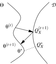
×Θ.Csisz´ar and Tusn´ady (1984) show that the EM algorithm can be derived as alternating mini-mization under the information divergence, as follows (see Figure 1):
Forward Step: Find the desired distribution Q(Xt+1)that minimizes the divergence from the previ-ous parameterθ(t):
Q(Xt+1)=argmin
QX∈D
Θ D
θ(t+1) θ∗
Q∗X
Q(Xt+1) θ(t)
Figure 1: A schematic representation of an iteration of the alternating minimization procedure. The square of the distance between a point inθinΘand a point QX in
D
indicates thediver-gence between them. The arrows indicate projection under this diverdiver-gence.
Backward Step: Find the parameterθ(t+1)that minimizes the divergence to Q(Xt+1):
θ(t+1)∈argmin
θ∈Θ
D(Q(Xt+1)||PX ;θ). (2)
In the language of Csisz´ar (1975), Q(Xt+1)is the I-projection of PX ;θ(t) onto
D
and is uniquely foundas Q(Xt+1)=PX|Y=y;ˆθ(t). The EM algorithm (Dempster et al., 1977; Wu, 1983) can be recovered easily
by substituting the I-projection into equation (2) and expanding the divergence using equation (1), to obtain
θ(t+1)
∈argmax θ∈Θ
EPX|Y
h
log pX(X ;θ)|y;ˆ θ(t)
i
. (3)
Note that we use the notationθ(t+1)∈argmin D(Q(t+1)
X ||PX ;θ)instead ofθ(t+1)=argmin D(Q(Xt+1)||PX ;θ)
because the backward step may not be unique.
We distinguish between the forward and backward steps of the alternating minimization proce-dure and the E and M steps of the EM proceproce-dure, as they are subtly different. The E step corresponds to computing the (conditional) expected log likelihood (EM auxiliary function) under the result of the forward projection. In practical implementations, the auxiliary function is not computed ex-plicitly in the E step – the expected sufficient statistics are all that need be computed. Thus, the E step corresponds to taking an expectation under the distribution found in the forward step. The backward projection minimizes the divergence from the result of the forward projection, while the M step maximizes the expected log likelihood computed in the E step (or alternatively, finds pa-rameters such that the sufficient statistics of the resulting model match those computed in the E step).
2.2 Generalized Alternating Minimization
Θ D
θ(t)
θ(t+1)
Q(Xt+1)
θ∗
Q∗X
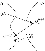
Figure 2: A schematic representation of an E step extension allowed by GAM algorithms corre-sponding to the M step extension of the GEM algorithm. In contrast to Figure 1, both the E and M steps reduce the divergence rather than minimizing it.
et al., 1999). We are interested in extending the alternating minimization formulation to such vari-ants by relaxing the requirement that the forward and backward steps perform exact minimization over the families of distributions. These generalized estimation steps are described as follows.
Generalized Forward Step: Find any desired distribution Q(Xt+1)that reduces divergence from the previous parameterθ(t):
QX(t+1): D(QX(t+1)||PX ;θ(t))≤D(QX(t)||PX ;θ(t)).
Generalized Backward Step: Find a parameterθ(t+1)that reduces the divergence to Q(Xt+1):
θ(t+1): D(Q(t+1)
X ||PX ;θ(t+1))≤D(QX(t+1)||PX ;θ(t)). (4)
Generalizations of the backward step correspond to the well known GEM algorithms. We allow similar generalization of the forward step. We refer to algorithms that consist of alternating ap-plication of such generalized forward and backward steps as generalized alternating minimization (GAM) algorithms. Thus, GAM algorithms allow for the expectation in the EM auxiliary function (equation (3)) to be found under the distribution Q(Xt+1)rather than PX|Y=y;ˆ θ(t). Q(Xt+1)is not chosen
arbitrarily; it must be closer to PX ;θ(t) than the desired distribution Q(
t)
X used at the previous
itera-tion. The effect of GAM iterations is to generate sequences of paired distributions and parameters
(Q(Xt),θ(t))that satisfy
D(Q(Xt+1)||PX ;θ(t+1))≤D(Q(
t)
X ||PX ;θ(t)).
Thus, we examine generalizations that are composed of forward and backward steps that reduce the divergence, as shown schematically in Figure 2.
2.3 Why GAM
posterior. This corresponds to extending the forward step to be a projection onto a subset of
D
which satisfies additional constraints (namely, belonging to a given parametric family), rather than a projection onto
D
itself.In the following example, which follows Jordan et al. (1999), we describe how the mean field approximation to the E step arises by further constraining the desired family
D
.Example 1 In the case of a Boltzmann machine, we have binary r.v.s X=S= (S1,···,Sn)modeled by the parametric family
pS(s;θ) =e∑
i<jθi jsisj+∑iθi0si
z(θ)
where z(θ) ensures PS;θ is properly normalized. Suppose the nodes 1,···,n of the Boltzmann
machine are partitioned into a set of evidence nodes E and a set of hidden nodes H, so that
Y =SE = (4 Si)i∈E. Then, given observations ˆsE of the evidence nodes, the forward step for EM
estimation of the Boltzmann machine is as follows.
Forward Step: Finding the desired distribution
Q(Xt+1)=argmin
QX∈D
D(QX||PX ;θ(t))
gives
q(SHt+,1SE)(sH,sE) =1sEˆ (sE)pSH|SE(sH|sˆE;θ(t))
where 1sEˆ (sE) =1 when sE =sˆE and 0 otherwise.
Note that a closed-form solution for the backward step is not generally available, but convergent algorithms can be obtained using gradient descent or iterative proportional fitting (Darroch and Ratcliff, 1972; Byrne, 1992). While the forward step can in principle be carried out exactly, this computation quickly becomes intractable as the number of states increases. In particular, direct computation of pSH|SE(sH|sˆE;θ(t))using Bayes rule involves a summation over all possible values
of the hidden nodes sH.
To get around this we define a subset of
D
consisting of mean field approximations to QSH|SE.That is, we define
D
MFto be those distributions inD
whose p.d.f. has the parametric formqS(s; µ) =1sEˆ (sE)
∏
i∈H
µsii (1−µi)1−si
| {z }
qSi;µi
where each µi takes values in[0,1]. Thus the members of
D
MF allow no dependencies betweennodes. It follows that a distribution QS∈
D
MF is fully specified by its parameter µ and the trainingobservations ˆsE.
The forward step can then be replaced by an approximate forward step, which is now a mini-mization over the variational parameter µ for fixedθ(t):
Approximate Forward Step: An (approximate) desired distribution
Q(Xt+1)∈argmin
QX∈DMF
with p.d.f.
q(St+1)(s) =1sEˆ (sE)
∏
i∈HqSi(si; µ(it+1))
is chosen by finding a variational parameter
µ(t+1)∈argmin
µ
D(QS;µ||PS;θ(t)).
As described by Jordan et al. (1999), this can be done directly, without needing to compute PSH|SE;θ(t), by solving the nonlinear system of mean field equations
µ(it+1)=σ
∑
jθ(t)
i j µ
(t+1)
j +θi0
!
,
whereσ(·)is the logistic function. Note that this simplification results from the careful craft-ing of the parametric form imposed on
D
MF.It can be seen that this variational EM variant is easily described in terms of minimizing the divergence between a constrained family of desired distributions and a model family. The approx-imate forward step in this example is a generalization of the usual I-projection onto
D
, and the resulting algorithm is therefore a GAM procedure.3. GAM Convergence
In this section, we describe our main result – a theorem which characterizes the convergence of GAM procedures. As the preceding example shows, some EM variants of interest are GAM pro-cedures but not GEM propro-cedures. This means that their convergence behavior may be different from what the familiar convergence properties of (G)EM would suggest. In particular, monotonic increase in likelihood and convergence to local maxima (technically, stationary points) in likelihood may no longer hold. This may happen even when the divergence is non-increasing, and when sta-tionary points of the likelihood are fixed points of the GAM procedure. We begin with a simple toy example where this can easily be seen.
Example 2 Let the complete random variable X = (X1,X2) represent the result of tossing a coin twice. That is, X1,X2are i.i.d., with Xi taking the value 1 with probabilityθand 0 with probability
1−θ. Let the incomplete random variable Y encode whether the result seemed “fair” or not. It takes on the value 1 if X takes on the values (0,1)or(1,0), and takes on the value 0 otherwise. Suppose the observation ˆy of Y is ˆy=0. In this simple case, the complete data likelihood is given
by
pX(x; θ) =θx1+x2(1−θ)2−(x1+x2)
and the incomplete data likelihood is given by
pY(y;ˆ θ) =pY(0;θ)
=pX(0,0;θ) +pX(1,1,;θ)
Note that the incomplete likelihood is convex, with global maxima atθ=0 andθ=1, and a global
minimum atθ=0.5. Desired distributions QX ∈
D
take the formqX(x) =
q11 if x= (1,1),
1−q11 if x= (0,0),
0 otherwise.
The divergence between a desired distribution and a model is given by
D(QX||PX ;θ) =q11log
q11
θ2 + (1−q11)log
1−q11
(1−θ)2,
which can be shown to be convex in q11for fixedθand convex inθfor fixed q11(though not jointly convex in q11 andθ). The EM algorithm for estimating θcan be given by a forward step and a backward step as follows:
Forward Step: As described above, the forward step is given by the I-projection of the model PX ;θ(t) onto
D. This is given by
q(Xt+|Y1)(x|yˆ) =pX|Y(x|y;ˆ θ(t)),
q(11t+1)= θ
(t)2
(1−θ(t))2+θ(t)2.
Backward Step: Minimizing the divergence given above overθfor a fixed q11gives
θ(t+1)=q(t+1) 11 . Thus, the EM iteration for this problem is
θ(t+1)= θ(t) 2
(1−θ(t))2+θ(t)2.
It can be seen thatθ(0)<0.5 gives convergence to the global maximum atθ=0.0, whileθ(0)>0.5 gives convergence to the global maximum atθ=1.0. Starting at the global minimum atθ=0.5
traps the algorithm there.
We now investigate how the additional constraint
0.4≤q11≤0.6 (5)
on the desired distribution changes the forward step, and as a result, the convergence behavior of the algorithm. Note that a forward step that projects onto this constrained set of desired distributions will reduce the divergence between the desired distribution and the model, and will therefore be a GAM procedure.
Computing the partial derivative
∂
∂q11D(QX||PX ;θ) =log q11
1−q11
1−θ
θ
shows that it is positive for 0.4≤q11≤0.6 whenθ< 1
1+√3/2≈0.4495. Therefore, the forward step from anyθ< 1
1+√3/2
is given by q11=0.4.
Suppose θ(0)=0.3. The unconstrained forward step would have given q(1)
11 =0.155, which would have violated the additional constraint (5). Under the additional constraint (5), the forward step is given by q(111)=0.4. This in turn leads toθ(1)=0.4, and the next forward step again gives q(112)=0.4, showing that the algorithm has converged in a single step, albeit to a value that is not
a maximum (or stationary point) in likelihood. Also, recall that the incomplete data likelihood is convex with a minimum atθ=0.5. This means that initial points inθ<0.4 will converge in one
step toθ=0.4, thereby reducing likelihood. Indeed, the likelihood at the initial point (θ=0.3) is 0.58 and the likelihood at the subsequent (limit) points (θ=0.4) is 0.52.
Thus, it is clear that the convergence behavior of GAM algorithms can differ extremely from that of EM algorithms, and therefore needs to be carefully studied. In fact, non-monotonic convergence behavior can also be seen in the case of incremental EM (Byrne and Gunawardana, 2000). In the following, we will show that under smoothness conditions on the forward and backward steps, GAM procedures that strictly reduce divergence at every step, except possibly at stationary points in likelihood, will yield solutions that are stationary points in likelihood.
3.1 GAM Convergence Theorem
The GAM convergence theorem is a direct application of the generalized convergence theorem (GCT) of Zangwill (1969). We will define the forward and the backward steps to be point-to-set maps, rather than functions, so that we may deal with extended E and M steps that do not yield unique iterates. The GCT will require that these maps be closed. Closedness of a point-to-set map is a smoothness property that is related to function continuity, and is defined as follows:
Definition 1 A point-to-set-map H : U→V is closed at u∈U if for any two sequences{u(t)}∞t=0∈U and{v(t)}∞t=0∈V the conditions u(t)→u, v(t)→v, and v(t)∈H(u(t)), imply that v∈H(u).
We now state Zangwill (1969)’s GCT:
Theorem 2 Let the point-to-set map H : Z→ Z determine an algorithm that given a point z(0) generates a sequencez(t) ∞t=0 through the iteration z(t+1)∈H(z(t)). Also let a solution setΓbe given. Suppose
(1) All points z(t)are in a compact set S⊆Z.
(2) There is a continuous functionα: Z→Rsuch that:
(a) if z6∈Γ, thenα(z0)<α(z)∀z0∈H(z),
(b) if z∈Γ, thenα(z0)≤α(z)∀z0∈H(z).
(3) The map H is closed at z if z6∈Γ.
We use this GCT to show our main convergence result for GAM procedures and then give a corollary that describes how they converge in likelihood.
Theorem 3 (GAM Convergence Theorem) Let
D
be any family of distributions on X and letΘ be the parameter family defined in Section 2. Let the solution setΓbe defined asΓ=
(
(QX,θ) : QX ∈argmin Q0
X∈D
D(Q0X||PX ;θ)andθ∈argmin
ξ∈Θ
D(QX||PX ;ξ)
)
.
Let FB :
D
×Θ→D
×Θbe any point-to-set map such that all(Q0X,θ0)∈FB(QX,θ)satisfy(GAM): D(Q0X||PX ;θ0)≤D(QX||PX ;θ)
with equality only if
(EQ): (QX,θ)∈Γ.
Let(Q(Xt),θ(t)) ∞
t=0∈
D
×Θbe a sequence generated from a pair(Q (0)X ,θ(0))by the iterative
ap-plication of the point-to-set-map FB:
(Q(Xt+1),θ(t+1))∈FB(Q(Xt),θ(t)).
Suppose thatΘis compact, that there is a compact set
D
0⊆D
such that(1) FB(
D
0×Θ)=4∪(QX,θ)∈D0×θFB(QX,θ)⊆D
0×Θ,(2) The point-to-set map FB is closed on
D
0×Θ,and that it can be shown that(Q(Xk),θ(k))∈
D
0×Θfor some iteration(k).Then all accumulation points(Q∗X,θ∗)of the sequence(Q(Xt),θ(t)) ∞
t=0lie in the solution setΓ and D(Q∗X||PX ;θ∗) =D∗and D(QX(t)||PX ;θ(t))→D∗.
Proof We restrict the point-to-set map FB to
D
0×Θ, and then apply Zangwill’s GCT above withS=Z=
D
0×Θ,α=D, H =FB, andz(t) ∞t=0=(QX(t),θ(t)) ∞t=k. The compactness of
D
0×Θfollows from the compactness of
D
0andΘindividually. The continuity of the divergence in(QX,θ)follows from the continuity of the divergence D(QX||PX ;θ) in QX and PX ;θ and the continuity of
pX ;θinθ. The theorem then follows by direct application of Zangwill’s theorem.
Corollary 4 (Stationary Points in Likelihood) In Theorem 3, suppose that
D
is the desired family defined in Section 2. Then the following hold for accumulation points(Q∗X,θ∗):(1) pY(y;ˆ θ∗) =e−D
∗
and pY(y;ˆ θ(t))→e−D
∗
.
Proof For(QX,θ)∈Γ, qX(x) =pX|Y(x|y;ˆ θ)so that D(QX||PX ;θ) =−log q(y;ˆ θ)yielding
conclu-sion (1).
Since(Q∗X,θ∗)∈Γ, q∗X(x) =pX|Y(x|y;ˆ θ∗), giving
θ∗∈arg min
θ∈Θ
D(PX|Y=y;ˆ θ∗||PX ;θ).
The divergence in the right hand side can be expanded as
D(PX|Y=y;ˆ θ∗||PX ;θ) =−log pY(y;ˆ θ) +D(PX|Y=y;ˆθ∗||PX|Y=y;ˆ θ). Taking the gradient of this expression and setting it to zero yields
−∇θlog pY(y;ˆ θ)θ=θ∗+∇θD(PX|Y=y;ˆθ∗||PX|Y=y;ˆ θ)θ=θ∗ =0. Since D(PX|Y=y;ˆ θ∗||PX|Y=y;ˆθ)is minimized whenθ=θ∗, this gives us that
∇θlog pY(y;ˆ θ)
θ
=θ∗ =0. This proves conclusion (2).
The GAM convergence theorem and corollary provide conditions under which iterative estima-tion procedures converge to staestima-tionary points in likelihood. However it is possible that these pro-cedures are not monotonic in likelihood. This can be see from the Pythagorean equality (Csisz´ar, 1975) which provides the following relationship between all QX in the linear family
D
and a modelPX ;θ
D(QX||PX ;θ) =D(QX||Q˜X) +D(Q˜X||PX ;θ)
where the I-projection ˜QX =argminQX∈DD(QX||PX ;θ)is uniquely specified as ˜QX|Y=yˆ=PX|Y=y;ˆθ.
From this we find the following relationship between the likelihood of the model estimates and the overall divergence
D(QX||PX ;θ) =D(QX ||PX|Y=y;ˆ θ)−log pY(y;ˆ θ).
While GAM procedures guarantee that D(Q(Xt+1)||PX ;θ(t+1))≤D(Q(Xt)||PX ;θ(t)), we can conclude
only that
log pY(y;ˆ θ(t+1))≥log pY(y;ˆ θ(t)) +∆(t)
where ∆(t)=D(Q(t+1)
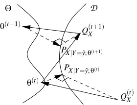
X ||PX|Y=y;ˆθ(t+1))−D(Q(Xt)||PX|Y=y;ˆ θ(t)). Since, as shown in Figure 3, this
quantity can be negative, it is possible for GAM algorithms to be non-monotonic in likelihood even while converging to local maxima in likelihood.
We now discuss the construction of a GAM mapping FB that satisfies the requirements of the GAM convergence theorem.
PX|Y=y;ˆθ(t) PX|Y=y;ˆθ(t+1) Θ
θ(t+1)
Q(Xt+1) D
Q(Xt) θ(t)
Figure 3: A schematic representation of how GAM procedures may be non-monotonic in likeli-hood. The solid arrows show forward and backward steps that reduce the divergence rather than minimizing it. The broken arrows show the forward steps that would have been taken by the EM algorithm (i.e., the I-projections of the models). Divergences that obey the Pythagorean equality are indicated by right triangles. In particular, the squared lengths of the broken arrows represent negative log likelihood. Note that the divergence between the desired distribution yielded by the forward step and the I-projection of the model decreases, while the negative log likelihood increases.
(1) F and B are closed on
D
0×Θ(2) F(
D
0×Θ)⊆D
0×Θand B(D
0×Θ)⊆D
0×ΘSuppose also that F is such that all(Q0X,θ0)∈F(QX,θ)haveθ0=θand satisfy
(GAM.F): D(Q0X||PX ;θ)≤D(QX||PX ;θ)
with equality only if
(EQ.F): QX =argmin Q00X∈D
D(Q00X||PX ;θ),
with QX being the unique minimizer. Suppose also that the point-to-set map B is such that all (Q0X,θ0)∈B(QX,θ)have Q0
X =QX and satisfy
(GAM.B): D(QX||PX ;θ0)≤D(QX||PX ;θ)
with equality only if
(EQ.B): θ∈argmin
ξ∈Θ
D(QX||PX ;ξ).
Then,
(1) the point-to-set map FB is closed on
D
0×Θ(2) FB(
D
0×Θ)⊆D
0×ΘProof If the point-to-set maps F : A→B and G : B→C are closed on A and B respectively, their
composition FG=G◦F is closed on A if B is compact. Since F and B are closed on
D
0×Θ, which is compact, it follows that FB is closed onD
0×Θ. That FB(D
0×Θ)⊆D
0×Θfollows directly from the assumptions of the proposition.The condition (GAM) follows directly from (GAM.F) and (GAM.B).
Conditions (EQ.F) and (EQ.B) together are not enough to ensure condition (EQ). Suppose
(RX,φ)∈FB(QX,θ). This implies that(RX,θ)∈F(QX,θ)and(RX,φ)∈B(RX,θ).
Suppose D(RX||PX ;φ) =D(QX||PX ;θ). Then (GAM.F) and (GAM.B) ensure that D(RX||PX ;φ) =
D(RX||PX ;θ) =D(QX||PX ;θ). Condition (EQ.F) gives
QX ∈arg min Q0
X∈D
D(Q0X||PX ;θ), (6)
RX ∈arg min Q0X∈D
D(Q0X||PX ;θ),
and (EQ.B) gives
θ∈arg min ξ∈Θ
D(RX||PX ;ξ). (7)
While equation (6) is the first criterion for membership inΓ, equation (7) is not quite the second cri-terion – the divergence minimized here is D(RX||PX ;ξ)instead of D(QX||PX ;ξ). Since by assumption,
QX is the unique minimizer of the divergence, QX =RX, giving the required condition
θ∈arg min ξ∈Θ
D(QX||PX ;ξ).
This allows us to construct a map FB through the composition of generalized forward and backward steps F and B. As seen in the proof it is insufficient for the forward and backward steps to satisfy the GAM and EQ conditions separately. It is also necessary for the forward step to satisfy the equality condition with a unique minimizer. For example, this condition is satisfied when
D
is defined by linear constraints as in Section 2 and the forward step is a simple projection, as in the case of EM. Even when this condition is not satisfied, it may be possible to show condition (EQ) for the composite map FB. It is important to show that FB strictly decreases the divergence for all points outside the solution setΓ, since any points where this does not hold are accumulation points of the algorithm.As an instance of the GAM procedure, EM convergence is also explained by these results as shown in Appendix A. The conditions of Theorem 3 and Corollary 4 are quite general, and very similar to those that must be satisfied to ensure GEM convergence (Wu, 1983). For example, in both GEM and GAM, condition (Q2) must hold. Insisting on this would rule out GMMs with parameter families that allow individual Gaussians to have a variance of zero. In practice, modeling considerations usually prevent such situations.
4. Incremental EM as GAM
saved from previous iterations. The statistics corresponding to the different partitions are pooled before performing the M step at each iteration, but the separate per-partition statistics are retained for use in future iterations. This algorithm has shown to give faster convergence in a number of applications (Digalakis, 1997; Thiesson et al., 2001; Hsiao et al., 2004), even though it may be non-monotonic in likelihood (Byrne and Gunawardana, 2000). Here, we use our GAM results to show that in most cases, the incremental updates do not sacrifice the convergence guarantees of EM, despite the non-monotonicity in likelihood. Note that Neal and Hinton (1998) have shown that incremental EM is monotonic in divergence, but not that it converges to EM fixed points.
The complete variable X = (X(1),···,X(n)) is assumed to consist of n independent compo-nents so that QX =∏ni=1QX(i). The visible variable Y = (Y(1),···,Y(n)) has observed value ˆy=
(yˆ(1),···,yˆ(n)). The components Y(i) are generated independently of each other, from their corre-sponding X(i).
The EM auxiliary function for these variables is
Φ(θ|θ(t)) = n
∑
i=1 EP
X(i)|Y(i)
h
log pX(i)(X(i);θ)|yˆ(i);θ(t)
i
= n
∑
i=1
Φ(i)(θ|θ(t)).
Rather than maximize this auxiliary function, the incremental EM algorithm allows re-estimation to be performed based on a single component ˆy(i)of the observation ˆy at any step. For example, in a
two-element problem the re-estimation procedure might proceed as follows :
θ(t+1)=argmax
θ∈Θ(Φ(1)(θ|θ(t−1)) +Φ(2)(θ|θ(t))), θ(t+2)=argmax
θ∈Θ(Φ(1)(θ|θ(t+1)) +Φ(2)(θ|θ(t))), θ(t+3)=argmax
θ∈Θ(Φ(1)(θ|θ(t+1)) +Φ(2)(θ|θ(t+2))), ···
This is not enough to ensure that Φ(θ(t+3)|θ(t+1))≤Φ(θ(t+1)|θ(t+1)) so the (G)EM convergence
results do not apply. However the algorithm can be formulated as an GAM procedure.
To show that incremental EM can be a GAM procedure, we describe it as a nested series of n incremental forward steps and n exact backward steps. Iteration(t+1)of incremental EM proceeds as follows. First, the iteration is initialized from the results of the previous iteration:
Q(Xt+1,0)=Q(Xt) and θ(t+1,0)=θ(t).
We then define a series of n incremental forward steps j=1,···,n
Q(Xt+(i)1,j)=
(
PX(i)|Y(i)=yˆ(i);θ(t+1,j−1) if j=i Q(t+1,j−1)
X(i) otherwise,
and backward steps
θ(t+1,j)∈argmin
ξ∈Θ
so that finally we set Q(Xt+1)=Q(Xt+1,n)and θ(t+1)=θ(t+1,n).
We formally represent the(j)thincremental forward step F(j):
D
×Θ→D
×Θas the singletonpoint-to-set map
F(j)(QX,θ) =
(
(Q0X,θ): Q0X =PX(j)|Y(j)=yˆ(j);θ
∏
i6=j
QX(i)
)
.
It updates the(j)thcomponent marginal Q
X(j)of QX but keeps the other component marginals fixed.
The backward step is represented by a closed point-to-set map B :
D
×Θ→D
×Θ satisfy-ing conditions (GAM.B) and (EQ.B) of Proposition 5 with Q0X =QX for(Q0X,θ0)∈B(QX,θ), andadditionally satisfying:
B(QX,θ)is a singleton set∀(QX,θ)∈
D
×Θ:(QX,θ)∈M(QX,θ). (8)Thus, we are guaranteed that θ0 =θ when D(QX||PX ;θ0) =D(QX||PX ;θ). This is equivalent to requiring that the EM auxiliary function has a unique maximizer. We note that this often holds in practice – for example, when the complete data distribution comes from a flat exponential family (Efron, 1975; Amari, 1995) as is the case with mixtures of Gaussians, or with hidden Markov models. Even when the complete data distribution is a curved exponential family, uniqueness can still be possible.
Using these composite maps we can describe incremental EM as
(Q(Xt+1),θ(t+1))∈FB(Q(t)
X ,θ(t))
where
FB=B◦F(n)◦ ··· ◦B◦F(1).
Proposition 6 As defined, incremental EM can be shown to converge to stationary points in likeli-hood through application of the GAM convergence theorem.
Proof For any (QX,θ) ∈
D
×Θ, we use the independence of the components X(i) and Y(i) todecompose the divergence D(QX||PX ;θ)into a sum of component divergences as follows
D(QX||PX ;θ) =
∑
iD(QX(i)||PX(i);θ).
The(j)thbackward step satisfies
D(Q(Xt+1,j)||PX ;θ(t+1,j))≤D(Q(Xt+1,j)||PX ;θ(t+1,j−1))
=
∑
i:i6=j
D(QX(t+(i)1,j−1)||PX ;θ(t+1,j−1)) +D(QX(t+(j)1,j)||PX ;θ(t+1,j−1))
where the right hand side has been expanded using the fact that the(j)th incremental forward step
leaves all but the(j)th component divergence unchanged. Since the(j)th incremental forward step
minimizes the(j)th component divergence,we get D(Q(Xt+1,j)||PX ;θ(t+1,j))≤
∑
i:i6=j
D(Q(Xt+(i)1,j−1)||PX ;θ(t+1,j−1)) +D(Q(t+1,j−1)
X(j) ||PX ;θ(t+1,j−1))
Condition (GAM) of Theorem 3 is therefore satisfied.
Since the maps F(j)and B are closed (Appendix A, Proposition 7), FB will be closed on
D
0, if the set is constructed so as to be compact (Appendix A). An appropriate definition ofD
0⊆D
is given in Appendix B along with a proof that incremental EM satisfies the equality condition (EQ) of Theorem 3.Thus, the GAM convergence theorem shows that incremental EM procedures converge to EM fixed points when the EM auxiliary function is uniquely maximized. However, it is not a GEM procedure, and monotonicity in likelihood is no longer guaranteed. Indeed, as discussed in Byrne and Gunawardana (2000) non-monotonicity in likelihood is observed in practice, and the conver-gence behavior is very different from that of (G)EM procedures, despite the common fixed point set. Thiesson et al. (2001) also show that the convergence behavior of incremental EM is different from that of EM in practice.
5. Variational EM as GAM
Variational approximations have been popular in cases where computing the exact forward step
qX(x) =pX|Y(x|y;ˆ θ)is intractable (Jordan et al., 1999). The idea is to restrict attention to a
subfam-ily
D
V ofD
such that members ofD
V have a particular parametric form, which is chosen so that projecting a model PX ;θontoD
V is more tractable than projecting it ontoD
. That is, aparametriza-tion qX(x; λ)withλ∈Λis fixed, and the family
D
V is defined asD
V ={QX ∈D
: qX(x) =qX(x;λ) for someλ∈Λ}.We assumeΛ⊆Rnis closed and bounded.
Then, the variational forward step is defined to be
FV(QX,θ) =
(
(Q0X,θ): Q0X ∈arg min
Q00X∈DV
D(Q00X||PX ;θ)
)
.
By the Pythagorean equality of Csisz´ar (1975),
D(Q00X||PX ;θ) =D(Q00X||PX|Y=y;ˆ θ) +D(PX|Y=y;ˆ θ||PX ;θ) =D(Q00X||PX|Y=y;ˆ θ)−log pY(y;ˆ θ).
Thus, Q00X ∈
D
V that minimizes this divergence also best approximates PX|Y=y;ˆ θ, which is the desireddistribution that would be chosen by the usual EM procedure.
Notice that the divergence minimized at every iteration is no longer just D(PX|Y=y;ˆ θ||PX ;θ)
(which is the negative log likelihood) as in the EM algorithm, and that therefore, the likelihood is not guaranteed to increase at every iteration. We now examine if the conditions of the GAM convergence theorem of Section 3 still hold if the forward step of the EM procedure is replaced by
FV.
First, note that
D
V is a natural choice forD
0as long as the set of variational parametersΛis com-pact. That the map FV is closed onD
V×Θfollows from Corollary 8 and Lemma 9 of Appendix A,of Proposition 5 (EQ.F) cannot be guaranteed in general, and must be verified for each choice of
D
V. If this condition holds, then the algorithm converges to minimizers of the divergence betweenthe family of variational approximations and the model family. For example, this happens when the variational E step is uniquely defined.
We now analyze when these limit points(Q∗X,θ∗)are stationary points in likelihood. Sinceθ∗
minimizes the divergence D(Q∗||PX ;θ)overθ,
∇θD(Q∗X||PX ;θ)
θ=θ∗ =0.
Expanding the divergence as before,
∇θD(Q∗X||PX|Y=y;ˆθ)
θ
=θ∗−∇θlog q(y;ˆ θ) θ
=θ∗=0
so that∇θlog q(y;ˆ θ)|θ=θ∗ =0 if and only if
∇θD(Q∗X||PX|Y=y;ˆθ)
θ=θ∗ =0.
Therefore aθ∗ generated by a variational EM procedure is a stationary point in likelihood if and only ifθ∗is a parameter that locally minimizes the variational approximation error. This can hap-pen in two ways. First, the variational error may have stationary points at stationary points in likelihood. This can only be ensured if the stationary points are known before estimation. Second, the variational error is independent ofθ. This is not possible if the variational family introduces independence assumptions that ensure tractability. In particular, a model which agrees with the variational approximation (e.g., a factorial HMM with parameter settings that decouple the state sequences) will have lower variational error than one that does not. We illustrate this in the case of the mean field approximation for Boltzmann machines.
Example 3 In Example 1, choose a pair of hidden nodes i,j connected by a dependency link. It is well-known (Byrne, 1992) that
∂ ∂θi j
log pS|SE(s|sˆE;θ) =sisj−EPS|SE[SiSj|sˆE;θ],
∂ ∂θk0
log pS|SE(s|sˆE;θ) =sk−EPS|SE[Sk|sˆE;θ] k=i,j,
which gives
∂ ∂θi j
D(Q∗S||PS|SE=sEˆ ;θ) =EQ∗
S[SiSj; µ]−EPS|SE[SiSj|sˆE;θ] =µ∗iµ∗j−EPS|SE[SiSj|sˆE;θ],
∂ ∂θk
If∇θD(Q∗S||PS|SE=sEˆ ;θ)
θ
=θ∗ is to be zero,
EPS|SE[SiSj|sˆE;θ∗] =EPS|SE[Si|sˆE;θ∗]EPS|SE[Sj|sˆE;θ∗]
must hold. This can only occur ifθ∗i j=0, when the model itself satisfies the constraints of the mean
field approximation. Thus, under this variational approximation, only Boltzmann machines where the hidden units do not depend on each other can give stationary points in likelihood.
To summarize, the GAM convergence theorem applies to variational EM in cases when the variational E step is uniquely defined. When this is so, the resulting model is at a local minimum of the divergence between the model family and the family of variational approximations. However, except in degenerate cases, this model cannot be at a stationary point in likelihood. These degenerate cases occur when the model satisfies the simplifying conditions that define the family of variational approximations. In this case, the variational EM algorithm is essentially performing standard EM over a restricted model family defined so as to be consistent with the variational approximations.
6. Conclusion
GAM iterative estimation procedures are a class of EM extensions whose E step can be varied in a manner analogous to the relaxation of the M step that occurs in GEM algorithms. We have provided conditions under which these procedures can be shown to converge to stationary points in likelihood. The conditions specify allowable E step variations that are in fact analogous to the M step variations that are allowed by GEM procedures. The convergence analysis is analogous to that presented by Wu (1983), but takes advantage of the information geometric framework of Csisz´ar and Tusn´ady (1984) to explicitly represent distributions in computing sufficient statistics.
We have analyzed the convergence behavior of two well known EM extensions, namely incre-mental EM and variational EM, as GAM procedures. Our GAM convergence analysis shows that incremental EM procedures converge to stationary points in likelihood, even though incremental EM is in general neither a GEM procedure nor monotonic in likelihood. Variational EM algorithms with unique E steps satisfy the conditions of the GAM convergence theorem but do not satisfy its corollary. Thus the GAM convergence theorem shows that such algorithms converge to solutions that minimize divergence, but these are not necessarily stationary points in likelihood. We then present an information geometric argument which shows that variational EM can only converge to stationary points in likelihood in degenerate cases.
Appendix A. EM Satisfies the GAM Convergence Theorem
Recall that the forward and backward steps F,B :
D
×Θ→D
×Θof the EM algorithm are given byF(QX,θ) =
(
(Q0X,θ): Q0X∈arg min
Q00
X∈D
D(Q00X||PX ;θ)
)
and
B(QX,θ) =
(
(QX,φ): φ∈arg min
ξ∈Θ
D(QX||PX ;ξ)
)
That the conditions (GAM.F), (GAM.B), (EQ.F), and (EQ.B) hold is obvious by construction. We will first show a compact
D
0that guarantees that F(D
0×θ)⊆D
0×θand B(D
0×θ)⊆D
0×θ. We will then show that F and B are closed onD
0×Θ. Proposition 5 then implies that the composite map FB satisfies the conditions of the GAM convergence theorem (Theorem 3).Restricting the desired family to a compact set We define
D
0asD
0=QX ∈D
: qX|Y(x|yˆ) =pX|Y(x|y;ˆ θ)for someθ∈Θwith
D
defined as in Section 2. Note that this forces every QX ∈D
0 to be the continuous mappingof someθ∈Θ. Therefore,
D
0 is the continuous mapping of the compact setΘ, and is therefore compact.By construction of
D
0, it is guaranteed that QX generated by a forward step will lie inD
0. Thus,F(
D
0×Θ)⊆D
0×Θ. By definition of B(·), B(D
0×Θ)⊆D
0×Θ.Closedness of the forward and backward steps The following proposition and corollary show that the minimization of a continuous function forms a closed point-to-set map. This implies that projection under the divergence forms a closed point-to-set-map, so that the (ungeneralized) forward and backward steps of the EM algorithm are in fact closed point-to-set maps.
Proposition 7 Given a real-valued continuous function f on A×B, define the point-to-set map F : A→B by
F(a) =arg min
b0∈B
f(a,b0),
={b : f(a,b)≤ f(a,b0)for∀b0∈B}.
Then, the point-to-set map F is closed at a if F(a)is nonempty.
Proof Let{a(t)}∞t=0and{b(t)}∞t=0be sequences in A and B respectively, such that
a(t)→a,
b(t)→b,
and suppose
b(t)∈Fa(t).
That is,
b(t)∈arg min
b0∈B
f(a(t),b0).
The map F is closed at a∈A if this implies that b∈F(a)– that is, that b∈arg min
b0∈B
f(a,b0).
To prove the proposition by contradiction, suppose b6∈arg min
b0∈B
f(a,b0). By assumption F(a)is
nonempty. Therefore, there exists ˆb∈arg min
b0∈B
f(a,b0). Chooseε>0 such that
By continuity of f(·,·)and f -monotonicity of(a(t),b(t)),∃K1such that
f(a(t),b(t))> f(a,b)−ε, ∀t>K1,
so that by equation (9),
f(a(t),b(t))> f(a,ˆb) +ε, ∀t>K1.
By continuity of f(·,ˆb)and f -monotonicity of(a(t),b(t)),∃K2such that
f(a,ˆb) +ε>f(a(t),ˆb), ∀t>K2.
Combining these two bounds gives∃t>K1,K2such that
f(a(t),b(t))>f(a(t),ˆb)
which is a contradiction since by assumption, b(t)∈arg min
b0∈B
f(a(t),b0), and therefore,
b∈arg min
b0∈B f(a,b
0),
b∈F(a).
Corollary 8 The point-to-set map F : A→B of Proposition 7 is closed on A if the set B is closed.
The following lemma shows that the Cartesian product of two closed point-to-set-maps is itself closed.
Lemma 9 Suppose F : A→B and G : A→C are closed to-set-maps. Then the product point-to-set-map H : A→B×C defined by
H(a) =F(a)×G(a)
is closed.
This follows by direct application of the definition of closedness of point-to-set maps.
Proposition 7 and the existence of the I-projection shows that the mapping fromΘto
D
defined byQX∈arg min Q0
X∈D
D(Q0X||PX ;θ)
Appendix B. Incremental EM: (EQ) and
D
0In this appendix, we show that incremental EM satisfies condition EQ of the GAM convergence the-orem, and show a compact restriction of the desired family that can be used to analyze convergence of incrmental EM.
B.1 Incremental EM Satisfies Condition (EQ)
(Q0X,θ0)∈FB(QX,θ)implies a sequence of incremental steps
(R(X0),φ(0)),···,(R(Xn),φ(n))
such that
(R(X0),φ(0)) = (Q
X,θ),
(R(Xj),φ(j))∈F(j)B(R(Xj−1),φ(j−1)), and
(Q0X,θ0) = (RX(n),φ(n)).
When D(Q0X||PX ;θ0) =D(QX||PX ;θ), the GAM inequality (already shown) gives that the
diver-gence is unchanged at every incremental step:
D(R(Xj)||PX ;φ(j)) =D(R(Xj−1)||PX ;φ(j−1))
for j=1,···,n. In fact, by conditions (GAM.F) and (GAM.B), the divergence is unchanged at each
incremental forward step F(j)and the backward step B:
D(R(Xj)||PX ;φ(j−1)) =D(R(Xj−1)||PX ;φ(j−1)) (10)
and
D(R(Xj)||PX ;φ(j)) =D(R(Xj)||PX ;φ(j−1)) (11)
for j=1,···,n. We will now show that QX(i) =PX(i)|Y(i)=yˆ(i);φ(i−1) for i=1,···,n and thatφ(j)=θ
for j=1,···,n, which will then imply that condition (EQ) holds.
To show QX(i)=PX(i)|Y(i)=yˆ(i);φ(i−1) we decompose equation (10) as
∑
i6=j
D(R(Xj()i)||PX ;φ(j−1)) +D(R(
j)
X(j)||PX ;φ(j−1)) =
∑
i6=j
D(R(Xj(−i)1)||PX ;φ(j−1)) +D(R(
j−1)
X(j) ||PX ;φ(j−1)).
Since R(Xj()i)=R (j−1)
X(i) for all i6= j at any incremental step(j), this reduces to
D(R(Xj()j)||PX ;φ(j−1)) =D(R(j−1)
for j=1,···,n. Since RX(j()j) =PX(j)|Y(j)=yˆ(j);φ(j−1) uniquely minimizes the component divergence D(RX(j)||PX ;φ(j−1))over all RX(j), this means that
R(Xj(−j)1)=R (j)
X(j) =PX(j)|Y(j)=yˆ(j);φ(j−1).
Thus, for any component(i), substituting in j=i and recalling that the first i−1 incremental E steps leave the component marginal RX(i) unchanged, we get
QX(i)=R(0)
X(i) =···=R (i)
X(i)=PX(i)|Y(i)=yˆ(i);φ(i−1) . (12)
We now show that φ(j)=θfor j=1,···,n. Since equation (11) tells us that the divergence
is unchanged at any backward step (j) , both PX ;φ(j) and PX ;φ(j−1) must minimize D(R(Xj)||·). By
assumption (8), the M-step is uniquely determined, so we must haveφ(j)=φ(j−1). We therefore
have the desired result
θ=φ(0)=···=φ(n)=θ0. Substituting this into equation (12) gives
QX(i)=R( 0)
X(i) =···=R (i)
X(i)=PX(i)|Y(i)=yˆ(i);θ.
Since this applies for all i=1,···,n, we have
RX(j)=PX|Y=y;ˆθ, ∀j=0,···,n.
In particular, QX =R(X0)=PX|Y=y;ˆ θ, which means that QX =argmin
Q00X∈D
D(Q00X||PX ;θ).
Since R(X1)=QX, we use equation (11) with j=1 and condition (EQ.B) on the backward map to get
θ∈argmin ξ∈Θ
D(QX||PX ;ξ).
This shows that condition (EQ) holds.
B.2 Definition of a Compact
D
0To find a suitable restriction
D
0 for any choice of Q(X0)∈D
, we first define the following sets of measures on the components X(i):D
INC(i) =nQX(i) : QX(i)=PX(i)|Y(i)=yˆ(i);θfor someθ∈Θo
∪nQ(X0()i)
o ,
and note that the continuity of PX|Y ;θ (assumed), and the compactness of Θ (assumed) give us
compactness of
D
INC(i) . We then define our restrictionD
INC0 ofD
byD
INC0 =(
QX : QX= n
∏
i=1
QX(i) for some(QX(1),···,QX(n))∈
D
INC(1) × ··· ×D
INC(n))