Inducing Grammars from Sparse Data Sets:
A Survey of Algorithms and Results
Orlando Cicchello [email protected]
Stefan C. Kremer [email protected]
Department of Computing and Information Science University of Guelph
Guelph, ON, Canada
Editor: Fernando Pereira
Abstract
This paper provides a comprehensive survey of the field of grammar induction applied to randomly generated languages using sparse example sets.
Keywords: Grammar Induction, Occam’s Razor, Finite State Automata, Abbadingo One Learning Competition
1. Introduction
This paper provides a survey of work conducted on inferring a class of randomly generated DFA (Deterministic Finite State Automata) from sparsely labeled example strings. Since the introduction of this class of problems to the grammar induction community, a number of solutions have been proposed. Our paper is the first comprehensive and comparative study of this interesting domain and is intended to fill the gap left by a lack of comprehensive introductory papers.
With this review, we hope to provide some background on the history of the problem and the motivation behind some of the leading algorithms. This includes a critical analysis of what leads to success and the necessary nomenclature for understanding the specific problem domain and its complexity.
We begin by presenting, in Sections 2 through 9, several key concepts and definitions of gram-mar induction. Included among the definitions is a simple example of how the training data for a specific class of grammar induction problems can be easily represented. The problem class, called
Abbadingo-style problems, was introduced in a 1997 DFA learning competition held to promote
new algorithms and to determine the limitations of learning DFA from sparse example data (Lang and Pearlmutter, 1997).
In order to understand the principles behind the current state of the art inference engine for
Abbadingo-style problems, we proceed in Section 10 with an overview of an algorithm proposed
sets. Although these benchmark data sets differ from the Abbadingo-style problems, they have been used to evaluate new inference techniques and are included for completeness. Some of these tech-niques can be carried over to other problem domains and therefore are essential in our review of relevant work.
2. General Definition of Grammar Induction
The general problem of grammar induction is defined as follows.
Definition 1 Given sets of labeled example strings S+and S−s.t. S+⊂L(G)and S−⊂L0(G)infer a DFA(A)such that the language of A denoted L(A) =L(G). L(G)is a language generated from an unknown Type-3 grammar(G). Its complement, L0(G), is defined as L0(G) =∑∗−L(G)where
∑∗is the set of all strings over the alphabet(∑)of L(G).
A more precise definition of the problem of learning Abbadingo-style DFA will be presented once we have covered most of the necessary nomenclature and problem specific details.
2.1 Type-3 Grammars
Only Type-3 grammars are considered for the above problem since the languages that they generate are precisely the sets accepted by Deterministic Finite State Automata (Hopcroft and Ullman, 1969). As defined by Harrison (1978), a Type-3 grammar is a four tuple:
G={T,N,P,S}
where
• T ⊆N is a finite non-empty set called the terminal alphabet of G,
• N is a finite non-empty set called the total vocabulary of G,
• P is a finite set of production rules,
• S∈(N−T)is referred to as the start state,
and the rules in P are of the form
• A→aB, or
• A→a,
where A,B∈N−T and a∈T .
2.2 Deterministic Finite State Automata
The Deterministic Finite State Automata (DFA) representing such grammars are quintuplets. Fol-lowing Hopcroft and Ullman (1969), a formal definition of a DFA(A)is given below:
A={Q,∑,δ,s,F}
where
• Q is a finite non-empty set of states,
• ∑is a finite non-empty set of input symbols or input alphabet,
• δ: Q×∑→Q the transition function,
• s∈Q the start state,
• F⊆Q the final states or accepting states of A.
The size of a DFA will be defined as the total number of states or elements in Q denoted|Q|.
3. Problem Domain
The DFA considered for inference (the target DFA) are Abbadingo-style DFA. In this paper, we fo-cus on a class of problems proposed by Lang, Pearlmutter, and Price (1998b), Lang and Pearlmutter (1997) as part of an international competition to promote new and better algorithms for inferring
Abbadingo-style problems. The generation process is driven by a nominal automaton size n which
allows the user to select an approximate number of states in the final automaton. The procedure for generating such problems operates as follows.
First, a random digraph with(5/4)n states is created. The 5/4 term was empirically developed
to generate automata which, after minimization, produce automata with approximately n states. (It is not know to what degree this method would work for automata with alphabets that are not binary.) Each state is given an out-going edge for every element of the input alphabet(∑)and a label of either accept or reject with equal probability. The start state(s)is chosen randomly with equal probability from the complete set of states(Q). Any state which is not reachable from s is discarded. Finally, after removing all unreachable states, the Moore minimization algorithm is applied to the DFA. If the resulting DFA does not have depth exactly (2log2n)−2 (rounded to the nearest integer) it is discarded and the procedure is repeated. The selection of automata with a particular depth was used to ensure fairness for the competition and subsequent experiments in which automata with greater depth are generally more difficult to learn.
The depth of a DFA is defined as the minimum number of transitions required to reach the furthest state from the start state. The depth constraint enforced on the generation of the target DFA ensures a set of problems whose relative difficulty remains consistent along the dimension of target size (Juill´e and Pollack, 1998b, Lang and Pearlmutter, 1997). Actually, the difficulty of the problem may be increased along two dimensions: (1) the size of the target DFA as mentioned above and (2) the sparsity of the training set(tr)defined as tr= (S+,S−).
4. Generating Positive and Negative Examples
The disjoint sets S+ and S− otherwise known as positive and negative exemplars respectively, are subsets of ∑∗ and are given to provide clues for the inference of the production rules(P) of the unknown grammar(G)used to generate the language(L). Creating sets S+and S− for
Abbadingo-style problems first requires using the target DFA to classify all strings (Stot) of length at most b(2log2n)+3cwhere n is the total number of states in the target DFA, as either accepted or rejected by G. If a string s is considered accepted by G then it is considered as part of the language of L, however, if string s is rejected by G then it is considered as part of the complementary language of
L, namely L0. Using a uniform distribution, a subset of the labeled strings are randomly chosen and added to either S+or S−depending on whether they have been classified as accepted or rejected by
G respectively. When we refer to the density (d) of the training data, we will be referring to the ratio of the complete set of all strings included in S+and S−such that
d= |S+|+|S−|
|Sb(2log2n)+3c
k=0 ∑
k|×100%
(see Definition 3). A completely labeled data set has a density of 100% when the training data sets
S+and S−include the complete set of all example strings up to a given length.
5. Augmented Prefix Tree Acceptor
The definition of an augmented prefix tree acceptor (APTA) will now be introduced in order to illustrate how sets S+ and S− may be dealt with simultaneously. Following the work of Coste and Nicolas (1997), an APTA with respect to S+and S−denoted APTA(S+,S−)is defined as a 6-tuple:
APTA ={Q,∑,δ,s,F+,F−}
where
• Q is a finite non-empty set of nodes.
• ∑is a finite non-empty set of input symbols or input alphabet, • δ: Q×∑→Q the transition function,
• s∈Q the start or root node,
• F+⊆Q identifying final nodes of strings in S+, • F−⊆Q identifying final nodes of strings in S−.
The size of an APTA will be defined as the total number of elements in Q denoted|Q|.
5.1 Example
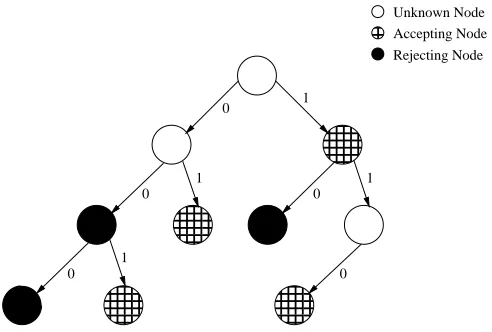
Consider sets S+={1,110,01,001} and S−={00,10,000}, the APTA with respect to S+ and S− or ATPA(S+,S−)is illustrated in Figure 1.
000
000
111
111
00
11
000
000
111
111
000
000
111
111
000
000
111
111
1
1 0
0 0
0
0 1
1
Rejecting Node Accepting Node Unknown Node
Figure 1: An incompletely labeled APTA of depth 3 representing sets S+={1,110,01,001} and
S−={00,10,000}.
respectively. The problem of inferring unknown DFA from example sets S+and S−can be reduced to simply contracting the APTA to directly obtain the target DFA. In other words, a minimization algorithm analogous to that of Hopcroft and Ullman (1969) can be used to identify equivalent nodes and merge them, thus simplifying the representation. If the APTA is complete, then the applica-tion of such an algorithm is straight-forward, but in our case it is not since only a fracapplica-tion of the complete data set is represented by the APTA. The absence of example strings results in undefined transitions and or labels within the APTA and consequently can carry over to the hypothesis DFA. It is important to note that merging nodes within the APTA places constraints on future merges, hence, the order with which the nodes are merged makes a difference. We now examine the issue of merging in more detail.
5.2 Merging for Determinization
In the previous section it was mentioned that pairs of equivalent nodes within the APTA may be merged to obtain a DFA. To clarify the phrase “equivalent nodes” the following recursive, contra-dictive definition has been included.
Definition 2 Two nodes qiand qjin the APTA are considered not equivalent iff:
1. (qi∈F+and qj∈F−)or(qi∈F−and qj∈F+), or
2. ∃s∈∑s.t. if(qi,s,qi0),(qj,s,qj0)∈δthen qi0 not equivalent to qj0
Such constraints maintain the property of determinism for the resulting DFA. For instance, this guarantees that each state within the hypothesis will have at most, one transition defined for each element of∑. This is crucial since any DFA containing a state with multiple transitions for any ele-ment in∑would no longer be a Deterministic Finite State Automaton but rather a Non-Deterministic Finite State Automaton (NFA).
The property of merging for determinization will become more apparent in the following sec-tions. The examples included clearly illustrate the constraints imposed on merging nodes within the APTA.
6. Occam’s Razor
At this point, we should note that there can be no single solution to the problem defined in Definition 1 since there are many DFA with different languages that are consistent with S+ and S− (Gold, 1967). Therefore, we need a method or inductive bias for selecting the “best” solution from many valid solutions in this under-constrained problem. It is for this reason that we adopt Occam’s Razor (Pitt, 1989) as an inductive bias for the inference process. Occam’s Razor simply states that entities
should not be multiplied unnecessarily. As an inference technique, we will take this to mean that
among competing hypothesis, the simplest is preferable (Pitt, 1989). From an information-theoretic stand-point, simplest could be interpreted as the least number of bits (Pitt, 1989). If so, Occam’s Razor would imply that the simplest hypothesis DFA would be that which has the least number of states since fewer states require less representation. We will refer to the smallest hypothesis DFA for a Type-3 Grammar(G)as the canonical DFA of(G).
7. Grammar Induction with Abbadingo-style Problems
We will now redefine the problem of grammar induction in the context of Occam’s Razor as an inductive bias. In particular we will use the following problem definition for an automaton with nominal size n.
Definition 3 Given sets of labeled example strings S+and S−s.t. S+⊂L(G)and S−⊂L0(G)infer a DFA(A)with the least number of states possible. L(G)is a language generated from an unknown Type-3 grammar(G). Its complement, L0(G), is defined as L0(G) =Sb(2log2n)+3c
k=0 ∑
k−L(G) where
Sb(2log2n)+3c
k=0 ∑k is the set of all strings of length at mostb(2log2n) +3cover the alphabet (∑)of
L(G)and n is the size of the canonical DFA of G.
8. Problem Complexity
If the “completely labeled” data set is available then an exact solution for a given Abbadingo-style problem can be obtained, in the limit, in polynomial time (Trakhtenbrot and Barzdin, 1973). The following definition is a natural interpretation of polynomial time limiting identification. It was initially introduced by Pitt (1989).
Let A be an inference algorithm for DFA. After seeing i examples, A conjectures some DFA Mi. We say that A makes an implicit error of prediction at step i if Miis not con-sistent with the(i+1)st example. (The algorithm is not explicitly making a prediction, but rather the conjectured DFA implicitly predicts the classification of the next example string). We propose the following as a definition of polynomial time identification in the limit. The definition is stated in terms of DFA, but may be applied to any inference domain.
Definition 4 DFA are identifiable in the limit in polynomial time iff there exists an inference algorithm(A)for DFA such that A has polynomial update time, and A never makes more than a polynomial number of implicit prediction errors. More specifically, there must exist polynomials p and q s.t. for any n, for any DFA M of size n, and for any presentation of M, the number of implicit errors of prediction made by A is at most p(n), and the time used by A between receiving the ith example and outputting the ith conjectured DFA is at most q(n,m1+...+mi), where mjis the length of the jth
example.
If however, the data set is incompletely labeled, then an approximating definition of learning is required. DFA were considered approximately learned when 99% or greater of the test data was correctly classified Lang and Pearlmutter (1997). Then, Occam’s razor serves as an inductive bias to the learning algorithm, under the assumption that minimum size automata also give maximum accuracy. The problem of minimum automaton identification from incompletely labeled training data has been proven to be NP-Complete (Gold, 1978). However, Lang (1992) and Freund, Kearns, Ron, Rubinfeld, Shapire, and Sellie (1993) have shown that the average case is tractable. In other words, randomly generated DFA can be “approximately learned” from sparse uniform examples within polynomial time.
9. Problem Space
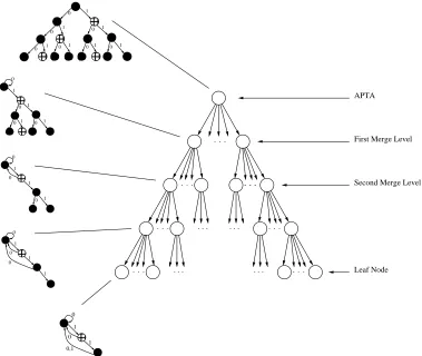
We will now introduce an extremely useful way of representing the problem space. Note, in this context, the term problem space will signify the complete set of all possible merge choices that exist in the APTA at any given point of the inference process. Similar to the APTA, the problem space can be conveniently represented as a tree which we shall refer to as the search tree (see Figure 2), but the two tree types should not be confused.
0
1
0
1
0
1
0
1
1 0
0
1 0 1 0 1 0 1 1 0 1 0
0
1
0
1
10 1 0 1 1 0 0
0
1
0
1
0
1
First Merge Level
Second Merge Level APTA Leaf Node 1 1 1 0 0 0 1 1 0 0,1 1 0 1 1 0 0 0
Figure 2: A representation of the problem space as a tree.
some state labels or transitions missing. Once a leaf node has been reached no other merge choices are available and an automaton matching the training set is obtained. Whether this automaton is a solution to the problem formulated in Definition 3 depends on the size of the automaton. Therefore, the inference engines used for DFA learning are essentially searching for the path that leads from the root of the search tree to the leaf node that represents the target DFA. In this sense, grammar induction can be viewed as a classical artificial intelligence tree search problem.
10. Induction on a Complete Data Set -Trakhtenbrot and Barzdin
The inference algorithm described in this section is the algorithm which was initially introduced by Trakhtenbrot and Barzdin (1973). It is very simple but effective in that it will produce the canonical DFA of any language for which it obtains the complete data set in polynomial time. A description of the algorithm is as follows.
10.1 Algorithm Description
• While visiting each proceeding node (λ) of the APTA in breadth-first order, compare the sub-tree rooted atλwith the sub-tree rooted at each node in the unique nodes list
• Ifλis pairwise distinguishable from each node in the unique list, appendλto the end of the list.
• Otherwise, disconnectλfrom the APTA by redirecting all transitions leading toλto point to the first node encountered from the list of unique nodes with whichλis indistinguishable.
10.1.1 EXAMPLE
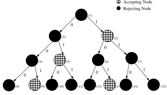
To illustrate how the algorithm works, consider the completely labeled APTA in Figure 3. The null string, represented by theεsymbol, which is a member of S− indicates a string of length zero. The label associated withεwithin the APTA is the label assigned to the root node. Hence, upon input of a string of length zero, according to the APTA in Figure 3, the target DFA will be in a rejecting state.
Each node within the APTA is assigned a number according to a breadth-first order. For in-stance, the root which would be visited first in a breadth-first traversal of the APTA is assigned the number 1 and the second node which would be visited in a breadth-first traversal of the APTA (the root’s left-most child) is assigned the number 2 and so on. The level order enumeration of the nodes is for the sole purpose of simplifying this example.
000
000
111
111
000
000
111
111
000
000
111
111
000
000
111
111
00
11
1 0 01 0 1 0 1 0 1
1 0 1
0
(8) (9) (11) (13) (14) (15)
(4) (5) (6) (7)
(2) (10) (12) (1) (3) Accepting Node Rejecting Node
Figure 3: A completely labeled APTA of depth 3, representing sets S+ and S− where S+ = {001,01,1,101}and S−={ε,0,00,000,010,011,10,100,11,110,111}.
unique nodes list (in this case just node 1). This involves, first comparing the label assigned to the root node (first node in the unique nodes list) with the label assigned to node 2. Since the labels are the same, we continue by redirecting the parent of node 2 to point to node 1. By doing this, we see from Figure 4 that the sub-tree rooted at node 2 is completely detached from the APTA. The idea is as follows, if there are no labeling conflicts within the sub-trees rooted at nodes 1 and 2, then node 2 and its descendants can be discarded, hence, reducing the size of the APTA. However, if there are labeling conflicts within the sub-trees rooted at nodes 1 and 2, the changes to the APTA must be undone and the next node in the unique nodes list is to be considered for merging with node 2.
000
000
111
111
000
000
111
111
000
000
111
111
000
000
111
111
1 0 1 10 0 1 0 1
1 0 1
0
0
(8) (9) (11) (13) (14) (15)
(4) (5) (6) (7)
(2)
(10) (12) (1)
(3)
Figure 4: The above figure is an illustration of the end result of redirecting the transition leading to node 2 from its parent (node 1) to the current node in the unique nodes list which is considered for merging (in this case node 1). The dotted arrows represent which nodes would be merged in the event that there are no labeling conflicts. For example, we see that nodes 8, 4, and 2 would merge with node 1, nodes 5 and 9 with node 3, and nodes 10 and 11 with nodes 6 and 7 respectively.
From Figure 4 we see that there are no labeling conflicts within the sub-trees rooted at nodes 1 and 2 and therefore, we need not consider for merging, node 2 with any other node within the list of unique nodes. In other words, the changes made to the APTA are kept and the sub-tree rooted at node 2 is discarded.
We now consider the next node (node 3) for merging with the first node (node 1) in the list of unique nodes. Since the labels differ, nodes 1 and 3 have rejecting and accepting labels respectively, merging these nodes is not possible. This forces us to consider for merging the next node in the list of unique nodes with node 3. However, since there are no other unique nodes to consider, we must promote node 3 as a unique node and append it to the list of unique nodes.
The next step is to consider merging node 6 with the first node (node 1) in the unique list. Since the sub-trees rooted at nodes 1 and 6 do not have any labeling conflicts, the transition leading from the parent node of node 6 remains pointing to node 1 and the sub-tree rooted at node 6 is discarded. This is illustrated in Figure 5.
000
000
111
111
000
000
111
111
10 1 0 1
1 0
0
(6) (1)
(3)
(7)
(12) (13) (14) (15)
Figure 5: The result of redirecting the transition leading from the parent node of node 6 to the root node (node 1).
where as, a 1 transition from the root node leads to an accepting node. Since there is a labeling conflict within the sub-trees rooted at nodes 1 and 7, and the labels of node 3 and 7 differ, we have no choice but to add node 7 to the list of unique nodes.
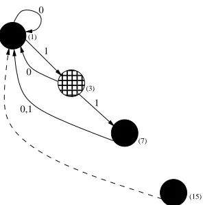
Finally, remaining are nodes 14 and 15. Since they are both leaf nodes, they will be merged with the first node within the unique list which shares the same label. For instance, nodes 14 and 15 will be merged with node 1 as illustrated in Figures 6 and 7.
The order in which nodes are considered for merging is very important here. Notice that even though nodes 14 and 15 could have been merged with node 7 they are not. Instead, these nodes are merged with the first node in the list of unique nodes to which they were determined to be equivalent.
000
000
111
111
1
1 1
0
0
0 (1)
(3)
(7)
(14) (15)
00
00
11
11
11 0
0
0,1 (1)
(3)
(7)
(15)
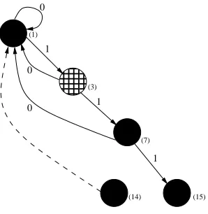
Therefore, the DFA represented by the APTA in Figure 3 is shown in Figure 8. There are many important concepts that are enforced in this example. For instance, the data set was complete for example strings of length 3. As stated in Section 8, if the complete set of example strings are available during the inference process, a solution can be obtained in polynomial time. Also, since the data set was complete there are no missing transitions or labels for any of the states within the final hypothesis DFA which is quite common when dealing with incomplete data sets. Perhaps what is more important to note here is that not only was a solution obtained for this example problem, but also the canonical DFA for the language represented by the example strings in S+and S−.
00
00
00
11
11
11
11 0
0
0,1 (1)
(3)
(7)
Figure 8: The final result obtained from performing the algorithm proposed by Trakhtenbrot and Barzdin on a completely labeled data set.
10.1.2 ADVANTAGES ANDDISADVANTAGES
Perhaps the biggest advantage of this algorithm is its simplicity. It provides a very simple and systematic approach to dealing with various size data sets in a very short time frame. Unfortunately, this has its disadvantage since the algorithm merges compatible nodes in breadth-first order despite the evidence or clues present within the training data. In other words, the attempted merge order is predetermined. The advantage of this is that very little search of the problem space is necessary to determine the next merge pair. Of course, this results in a fast running algorithm with very little over head. However, this does not make efficient use of the evidence or clues in the training data. It is important to note that the advantages and disadvantages outlined above apply not only to the algorithm proposed by Trakhtenbrot and Barzdin (1973) for compete data sets but also for the modified version of this algorithm which is able to deal with incomplete training data.
10.1.3 THERUNNINGTIME
The upper bound on the running time of this algorithm is mn2, where m is the total number of nodes in the initial APTA and n is the total number of states in the final hypothesis (Lang, Pearlmutter, and Price, 1998b).
11. Lang 1992 -The Average Case is Tractable
exam-ples. The modifications made to the algorithm were needed to maintain consistency with incomplete training sets. For instance, unlabeled nodes and missing transitions in the APTA needed to be con-sidered.
11.1 Dealing with Incomplete Data Sets
The simple extensions added to the Trakhtenbrot and Barzdin algorithm are summarized as follows. If node q2is to be merged with node q1then;
• labels of labeled nodes in the sub-tree rooted at q2, must be copied over their respective unlabeled nodes in the sub-tree rooted at q1.
• transitions in any of the nodes in the sub-tree rooted at q2that do not exist in their respective node in the sub-tree rooted at q1, must be spliced in.
As a result of these changes, the Traxbar algorithm will produce a (not necessarily minimum size) DFA that is consistent with the training set (Lang, 1992).
Experiments with the algorithm were conducted on randomly generated problem sets which consisted of target DFA and training data which varied in size and density. The variations in the problem sets allowed Lang (1992) to make several observations of how well the Traxbar algorithm performs on problems which vary in difficulty.
11.2 Training Data Density
One of the experiments conducted by Lang (1992) examined how the Traxbar algorithm performs as the training data density varied from approximately 0 to 5 percent. The generation of the 512 state target DFA used in these experiments are described in the following section.
11.2.1 GENERATION OF THEPROBLEMSETS
The target DFA which were roughly 512 states were constructed from randomly generated 640 state DFA. Each state of the 640 state DFA was assigned a 0 and 1 out-going transition with random destinations. Each state was then assigned an accepting or rejecting label with probability 0.5. Any states not reachable from the start state were removed. Finally, the DFA were then minimized with the Moore minimization algorithm. Any of the resulting DFA that did not have a depth of 16 were discarded.
For the 1000 learning trials, the size of the training data ranged from 200 to 200000 examples strings. The construction of the data set first involved generating all binary strings of length 0 to 21 and then, without replacement, randomly selecting example strings which were to be assigned a label according to the target DFA.
11.2.2 RESULTS
The experiments showed that as the density of the training data varied, the performance of the learning algorithm went through three distinct states.
Stage 2: As the training data density varied within the range of 1.5 to almost 3 percent, it was observed that smaller hypotheses (only 10 percent greater than the target DFA) were being generated and the generalization on the test data improved significantly, achieving classifica-tions of about 99.9 percent accuracy.
Stage 3: Once the training data density reached about 3 percent, the hypotheses were approxi-mately the correct size and the generalization achieved ranged from 99.99 to 99.999 percent accuracy. It was observed that increasing the density of the training data beyond 3 percent had little effect on the accuracy of the generalization.
11.3 How Performance Scales with Target Size
Another experiment conducted by Lang (1992), examined how the requirement of training data changes as the number of states in the target DFA varies. There were 2000 learning trials conducted for each of the 6 problem sets. The average size of the target DFA for the 6 problem sets were 31.9, 63.9, 127.4, 254.8, 510.7, and 1020.5 states. The generation of the target DFA involved extracting the sub-graph reachable from a randomly selected start state of a randomly generated degree-2 digraph consisting of (5/4)n states. As with the first experiment, if the depth of the target DFA was not 2log2n−2 it was discarded.
11.3.1 RESULTS
From these experiments, several observations were made.
1. For good generalization, doubling the size of the target DFA required that the training data be increased by a factor of roughly 3.
2. For target DFA increasingly large, the requirement for training set density approaches 0.
11.4 Summary
Gold (1978) showed that exact identification of DFA from sparsely labeled example strings is NP-Complete, but Lang (1992) demonstrated experimentally that the average case is tractable, while Freund, Kearns, Ron, Rubinfeld, Shapire, and Sellie (1993) actually proved that the average case is polynomial, albeit with an enormously less efficient algorithm. In other words, approximate identification of DFA from sparsely labeled example strings is possible in polynomial time. Also, Lang (1992) has identified boundaries on the density of the training sets required for a specific class of DFA learning problems.
In addition to exploring the boundaries of inducing DFA from sparsely labeled training data and examining the amount of training data required for various size DFA, Lang (1992) introduced a method of consistently producing DFA to which the inference capabilities of future algorithms can be compared. For instance, the enforced proportion of the number of states relative to the depth of the DFA maintains a consistent level of difficulty for learning DFA. This restricted set of DFA sets a standard for which future algorithms can be tested relative to each other.
12. Abbadingo One DFA Learning Competition
In 1997, Kevin J. Lang and Barak A. Pearlmutter held a DFA learning competition. The competition presented the challenge of predicting, with 99% accuracy, the labels which an unseen DFA would assign to test data given training data consisting of positive and negative examples. As described by Lang, Pearlmutter, and Price (1998b), Lang and Pearlmutter (1997), there were 3 main goals of the competition. The first was to promote the development of new and better algorithms. The second was to present to the machine learning community problems which lie beyond proven bounds with respect to the sparseness of the training data and to collect data regarding the performance of a variety of algorithms on these problems. Finally, the third goal of the competition was to provide a consistent means of comparing the effectiveness of new and existing algorithms for learning DFA.
12.1 How the Problems were Generated
A DFA with a nominal size of n states was generated according to Section 3. Each of the possible 16n2−1 binary strings whose length ranged from 0 to 2log2n+3 where classified according to the DFA. The training set and the test set were then uniformly drawn without replacement from the complete set of labeled binary strings according to the desired density. Participants only had available to them the labeled training set and an unlabeled test set which they were expected to label and later submit for evaluation. Competition winners consisted of those participants who where the first to solve a problem which was not dominated by other solved problems.
12.2 The Dominance Rule
The dominance rule (Lang and Pearlmutter, 1997) exercised during the competition stated that a problem x is dominated by a problem y when either or both of the following held true.
1. the training set for y is less dense than the training set for x
2. the number of states of the target DFA for problem y is greater than that of problem x.
12.3 Results
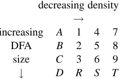
The dominance rule allows for multiple winners. In fact, there were two winners of the Abbadingo One Learning Competition, Rodney Price for solving problems R and S and Hugues Juill´e for solv-ing problem 7. The competition consisted of 16 problems in total, 4 (A, B, C, and D) were for practice only and had been previously solved by the Traxbar algorithm and the remaining 12 where the official challenge problems. A summary of the 16 problems and the competition results are found in Table 1.
The official challenge problems consisted of 3 distinct groups. Each group mainly differed in the sparseness of the training sets. For example, each group contained DFA that ranged in size from approximately 65 to 512 states, however, the training sets were significantly less dense for the third group of problems such that 8, 9, and T remained unsolved.
Problem Solved By Target Size Target Depth Training Set Size
A - 61 10 4456
B - 119 12 13894
C - 247 14 36992
D - 498 16 115000
1 Juill´e 63 10 3478
2 Juill´e 138 12 10723
3 Price 260 14 28413
R Price 499 16 87500
4 Juill´e 68 10 2499
5 Juill´e 130 12 7553
6 Juill´e 262 14 19834
S Price 506 16 60000
7 Juill´e 65 10 1521
8 unsolved 125 12 4382
9 unsolved 267 14 11255
T unsolved 519 16 32500
Table 1: Problems and results obtained from http://abbadingo.cs.unm.edu of the 1997 Ab-badingo One Learning Competition
decreasing density →
increasing A 1 4 7
DFA B 2 5 8
size C 3 6 9
↓ D R S T
12.4 Price’s Winning Algorithm
Price was able to win the Abbadingo One Learning Competition by using an evidence driven state merging (EDSM) algorithm. Essentially, Price realized that an effective way of choosing which pair of nodes to merge next within the APTA would simply involve selecting the pair of nodes whose sub-trees share the most similar labels. Since every label comparison could reveal the incorrectness of the merge, on average, a merge that survives more label comparisons is most likely to be correct (Lang, Pearlmutter, and Price, 1998b).
12.5 Post-Competition Work
A post-competition version of the EDSM algorithm as described by Lang, Pearlmutter, and Price (1998b) is included below.
12.5.1 ALGORITHM DESCRIPTION
• Evaluate all possible pairings of nodes within the APTA.
• Merge the pair of nodes which has the highest calculated score. The score is calculated by assigning one point for each overlapping labeled node within the sub-trees rooted at the nodes considered for merging.
• Repeat the steps above until no other nodes within the APTA can be merged.
12.5.2 ADVANTAGES ANDDISADVANTAGES
The general idea of the EDSM approach to merge pair selection is to avoid bad merges by selecting the pair of nodes within the APTA which has the highest score. It is expected that the scoring will indicate the correctness of each merge, since on average, a merge that survives more label comparisons is most likely to be correct (Lang, Pearlmutter, and Price, 1998b). Unfortunately, the difficulty of detecting bad merge choices increases as the density of the training data decreases. Since the number of labeled nodes decreases within the APTA as the training data becomes more sparse, the idea of selecting merge pairs based on the highest score proves less effective. This explains why the EDSM approach did well with large automata but not as well with low density problems.
Unlike the Traxbar algorithm introduced earlier, the EDSM approach for DFA learning relies on the training data to select its merge order. For instance, the order in which nodes are merged is directly dependent on the number of matched labels within the sub-trees rooted at each node. On the other hand, the Traxbar algorithm attempts to merge nodes in a predefined order despite the available evidence in the training data. The restriction on the merge order results in a trade-off of accuracy for simplicity and fast performance. It is the performance that is the biggest disadvantage to the EDSM approach in that it is not very practical for large problems. Considering every potential merge pair at each stage of the inference process is computationally expensive.
12.6 Windowed EDSM (W-EDSM)
12.6.1 ALGORITHM DESCRIPTION
• In breadth-first order, create a window of nodes starting from the root of the APTA. The recommended size of the window is twice the number of states in the target DFA.
• Evaluate all possible merge pairs within the window.
• Merge the pair of nodes which has the highest number of matching labels within its sub-trees. • If the merge reduces the size of the window, in breadth-first order, include the number of
nodes needed to regain a window of size twice the number of states in the target DFA.
• If no merge is possible within the given window, increase the size of the window by a factor of 2.
• Terminate when no merges are possible.
12.6.2 ADVANTAGES ANDDISADVANTAGES
As should be expected, the running time of the W-EDSM algorithm is much better than that of EDSM. The improvement in the running time is due to the reduction of the search space at each merge step of the algorithm. Of course, this can hurt the performance of the algorithm in that rel-atively rare, high scoring merges involving deep nodes may be excluded from the window (Lang, Pearlmutter, and Price, 1998b). For instance, the ideal algorithm would consider all possible merge pairs and select for merging, the pair of nodes which scores highest. Since such an algorithm is com-putationally expensive, only a subset of possible merge pairs are to be considered. This, of course, presents the task of selecting the correct set of nodes to be included within the window. Similar to Traxbar, nodes are included within the window based on a breadth-first order. Unfortunately, this selection process does not include nodes based on the evidence within the training data, hence, limiting the success of the algorithm to problems that favour windows which grow in breadth-first order.
Another problem with the W-EDSM algorithm is that a recommended window size of twice the target DFA be used. If the size of the target DFA is not known then this could be a problem. However, a simple solution could include executing the algorithm several times while gradually increasing the window size. Unfortunately, this has it’s problems also since you do not know exactly when to stop increasing the window size.
12.6.3 THERUNNINGTIME
It is conjectured that a tight upper bound on the running time of the W-EDSM algorithm is closer to
m3n than to m4n where m is the number of nodes in the APTA and n is the number of states in the
final hypothesis (Lang, Pearlmutter, and Price, 1998b).
12.7 Blue-Fringe EDSM
12.7.1 ALGORITHM DESCRIPTION
• Colour the root of the APTA red.
• Colour the non-red children of each red node blue. • Evaluate all possible pairings of red and blue nodes.
• Promote the shallowest blue node which is distinguishable from each red node. Break ties randomly.
• Otherwise, merge the pair of nodes which have the highest number of matching labels within their sub-trees.
• Terminate when there are no blue nodes to promote and no possible merges to perform.
12.7.2 ADVANTAGES ANDDISADVANTAGES
Similar to the W-EDSM algorithm, Blue-Fringe EDSM places a restriction on the merge order. For example, the algorithm always starts with the root node coloured red and its children blue resulting in a maximum of 2 possible merge pairs to choose from at the start. Considering the sparseness of some of the data sets, one would assume that the pool of possible merge pairs should be greatest from the start and then gradually decrease to save on the running time. This appropriately considers all the evidence within the training data at the start which ideally would contribute in making the correct decisions in the initial stage of the algorithm. This is important since changing the label of a node after it has been labeled as a result of a merge isn’t possible within this algorithm. Instead, as the algorithm progresses, the number of red and blue nodes increases resulting in a larger number of possible merge choices. Despite the restriction in the merge order and the reduction in merge choices at each merge level within the search tree, Blue-Fringe EDSM is very effective and its inference capabilities are comparable to those of W-EDSM.
12.7.3 THERUNNINGTIME
The upper bound on the running time of the Blue-Fringe EDSM algorithm is mn3 where m is the total number of nodes and n is the total number of states in the initial APTA and final hypothesis respectively (Lang, Pearlmutter, and Price, 1998b). It is important to note that this is of an order of magnitude greater than the Traxbar algorithm.
12.8 Juill´e’s Winning Algorithm
The inference engine used by Hugues Juill´e is vastly different than the algorithms discussed thus far. Actually, Juill´e and Pollack are the first to use random sampling techniques on search trees as a heuristic to control the search (Juill´e and Pollack, 1998a). The idea of using a tree to visualize the search space is very practical (see Section 9).
12.8.1 SAGE
The algorithm is based on a Self-Adaptive Greedy Estimate search procedure (SAGE). Each iter-ation of the search procedure is composed of two phases, a construction phase and a competition
It is in the construction phase where the list of alternatives or merge choices is determined. All the alternatives in the list have the same depth within the search tree. Each member of a population of processing elements is then assigned one alternative from the list. Each processing element then scores its assigned alternative by randomly choosing a path down the search tree until a leaf node is reached or a valid solution is encountered. Next, the competition phase kicks in.
The scores assigned to each alternative in the search tree are then used to guide the search. The meta-level heuristic determines whether to continue with the next level of search. If so, each processing element is randomly assigned one of the children of it’s assigned alternative. The search ends when no new node can be expanded upon.
To avoid an exhaustive search of the problem space only the first set of initial merges are ex-plored. These are thought of as the most critical merge choices since each merge places constraints on future merges.
12.8.2 ADVANTAGES ANDDISADVANTAGES
The random selection of merge pairs at a given level of the search tree results in a fast technique for obtaining an hypothesis DFA. Since there is no need for managing a window of merge pairs there is a savings in computation. In addition, this provides an unbiased exploration of the problem space. However, selecting merge pairs at random ignores the clues in the training data and results in a lot of unnecessary searching. This approach is thus, much more computationally intensive than the EDSM algorithm and its derivatives. More search results in a greater demand on CPU time and in that respect, an implementation of SAGE on large problems is not very realistic unless it is designed for a system with a highly parallel architecture. For instance, Juill´e and Pollack (1998b,a) conducted several simulations on a network of Pentium PCs and SGI workstations. This is in sharp contrast to the EDSM simulations mentioned above which were implemented on desktop computer equipment. In effect, the portability of the SAGE inference engine is far more limited than the others mentioned previously.
12.9 Exploring the Search Space Using the EDSM Approach
Experimenting with the ideas incorporated in SAGE, Lang (1998) introduced several new algo-rithms which use the idea of exploring the search space combined with the EDSM approach. These algorithms consist of a generic outer loop that supplies a binary control string to a base algorithm. Each time the base algorithm is run, a modified control string is used to guide the base algorithm in it’s search. For example, when a 0 bit is encountered in the control string the base algorithm makes the same choice as the original algorithm, however, if a 1 bit is encountered the choice of the original algorithm is not made and is considered as invalid for the remainder of the run (Lang, 1998). According to Lang (1998), the results obtained from the application of the new algorithms on
Abbadingo-style problems are the best ever and use far less computation than the SAGE algorithm.
In later work, Lang (1999) describes an implementation of these ideas. The resultant algorithm (Ed-beam) consisted of the outer loop described above wrapped around the Blue-Fringe algorithm.
12.9.1 ADVANTAGES ANDDISADVANTAGES
of labeled nodes decreases within the APTA, the matching labels heuristic generates more ties. Since ties are broken randomly, the effectiveness of the heuristic quickly diminishes. Lang (1998) indicates Juill´e replaced the random merge pair selection heuristic in SAGE with the matching labels heuristic during the Abbadingo One Learning Competition to solve problem 7 of the benchmark problem set.
12.10 A New Limited Search Approach to Learning Abbadingo-style DFA
Recent work by Cicchello and Kremer (2002b), Cicchello (2002) has lead to a new and more ef-ficient method of searching the problem space. Instead of performing an exhaustive search over the initial set of merges of the inference process as does Ed-beam (see Subsection 12.9), Cicchello and Kremer (2002b), Cicchello (2002) suggest focusing on choosing an alternative first merge. The new algorithm (TBW-EDSM) was inspired by the results obtained from evaluating the importance of choosing an alternative merge choice to that of the matching labels heuristic on one of the first 5 levels of the search tree (Cicchello and Kremer, 2002a). Realizing that the potential for improve-ment is greatest when altering just the first merge, Cicchello and Kremer (2002b), Cicchello (2002) incorporate a breadth-first traversal of the available first merges and perform the remaining merges in the order suggested by the matching labels heuristic. Since a breadth-first merge order considers the largest trees of suffixes first, it is expected that on average the most changes in the form of splic-ing transitions and labelsplic-ing of unlabeled nodes within the APTA will occur. By maksplic-ing a sufficient amount of correct changes to the APTA on the first merge, the matching labels heuristic will be better able to select the order of the remaining merges. The argument behind this assumption is as follows. Sparser data sets result in fewer labeled nodes within the APTA for a given problem. Fewer labeled nodes implies rare high scoring merge pairs and more ties. Since ties are broken ran-domly, the effectiveness of the matching labels heuristic quickly becomes comparable to randomly choosing merge pairs at the beginning of the inference process. Therefore, we must introduce new and better ways of selecting the initial merges. One way to do so is by using the breadth-first merge order as implemented in the TBW-EDSM algorithm.
12.10.1 ADVANTAGES ANDDISADVANTAGES
An advantage of the TBW-EDSM algorithm is that it avoids exhaustively searching through the initial merge of the inference process. Since the order of the first merge is predefined, maintaining a window of nodes and evaluating each possible merge pair is not necessary. This results in an improvement on the running time of the W-EDSM algorithm. However, the biggest disadvantage of the TBW-EDSM algorithm is that there may not exist a first merge which makes enough changes to the APTA. Under this condition, additional search may be required in other levels of the search tree.
12.11 Summary
13. Induction of Small DFA
The focus thus far has been on algorithms that have been evaluated using Abbadingo-style problems. The benchmark problem sets introduced in this section do not posses the consistency in the dimen-sion of training set density and DFA size with respect to depth as do the Abbadingo problem sets. However, some of the inference techniques introduced in the inference engines developed to deal with smaller problem sets can be carried over to other problem domains and therefore are included.
14. Tomita Grammars
Prior to to the work of Lang (1992), an accepted benchmark set of Grammars used for induction were those presented by Tomita (1982). As initially presented by Tomita (1982), the seven gram-mars are;
1. 1∗
2. (10)∗
3. any string without an odd number of consecutive 0’s after an odd number of consecutive 1’s.
4. any string without more than 2 consecutive 0’s.
5. any string of even length which, making pairs, has an odd number of (0 1) or (1 0)’s.
6. any string such that the difference between the numbers of 1’s and 0’s is 3n.
7. 0∗1∗0∗1∗
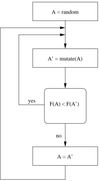
Tomita Grammars can be represented by DFA ranging in size from 3 to 6 states. In comparison to the Abbadingo-style problems, the DFA representing these grammars are very small and permit the use of inference engines that are computationally more expensive. As an example, consider the hill-climbing algorithm introduced by Tomita (1982). The initial step of the algorithm involves constructing a random n state DFA. A copy of the DFA is then made and mutated by randomly choosing one of the following operations.
• removing a transition • inserting a transition
• changing the destination of a transition to another destination • converting an accepting state to a rejecting state and vice versa
Both DFA are evaluated by a scoring function. The DFA which achieves the best score is kept while the other is discarded. The scoring function used to evaluate the DFA is r−w where r is the
number of example strings in S+ classified correctly and w is the number of example strings in S− classified incorrectly. A flowchart of the algorithm can be seen in Figure 9.
yes
no A’ = mutate(A)
A = random
A = A’ F(A) < F(A’)
Figure 9: Flowchart of Tomita 1992 hill-climbing algorithm.
problems and the Tomita Grammars are relatively simple to infer, the contribution made by Tomita (1982) has had a positive impact on the development of new algorithms. For example, Giles, Chen, Miller, Chen, Sun, and Lee (1991), Pollack (1991), Forcada and Carrasco (1995), Dupont (1994), Luke, Hamahashi, and Kitano (1999), Bengio and Frasconi (1995) have incorporated the Tomita Grammars in evaluating the performance of their inference engines. The algorithms introduced in these papers describe applications of Genetic algorithms and Second-Order Recurrent Networks for rule induction. The introduction of the Tomita Grammars to the grammar induction community brought attention to the fact that there was a need for a benchmark problem set for comparing the effectiveness of various inference engines.
15. Exact DFA Inference with the Aid of Backtracking
Another benchmark problem set that has been used in the development of new algorithms is that which was used to evaluate exact DFA learning algorithms by Lang (1999). Earlier versions of the benchmark problem set were introduced by Oliveira and Silva (1998) and Oliveira and Edwards (1996). The benchmark problem set used by Lang (1999) consisted of 810 problems1. Each problem was generated by using an unknown Moore machine having between 4 and 21 states to label 20 binary strings of length 30. The training data consisted of not 20 labels, one label for each string,
but rather a label for each state that was visited throughout each of the strings. The objective was to infer a minimum size DFA consistent with each training set.
The DFA learning algorithms evaluated using the benchmark problem set described above in-corporated a new concept which was first proposed by Beirmann and Petry (1975). The concept is backtracking and is included in MMM an exact DFA learning algorithm presented by Oliveira and Edwards (1996).
15.1 MMM
The algorithm begins with a one state hypothesis DFA. The hypothesis is expanded upon by com-paring transitions within to transitions in the APTA. For example, every node within the APTA is mapped to a state in the hypothesis DFA. If there exists a transition from a node in the APTA which is absent in its corresponding state in the hypothesis DFA, the transition is added and is directed to either one of the existing states or to a new one. If the corresponding transition is present, it is tested for consistency with the APTA. In the event that the hypothesis DFA is inconsistent with the APTA, the last choice made is undone. Otherwise, the algorithm continues.
15.2 Bica
A more constructive approach to resolving the inconsistencies within the hypothesis DFA and the APTA was introduced by Pena and Oliveira (1998). Instead of just undoing the last choice made as is the case with MMM, Pena and Oliveira (1998) suggest trying to determine which decision(s) made earlier on is responsible for the current inconsistencies between the hypothesis DFA and the APTA. By determining which move is the cause of the impasse, a jump to this point within the search tree may be made and the branch of the search space rooted at this point can be ignored for the rest of the search. These jumps are called non-chronological backtracks or back-jumps (Russel and Norvig, 1996). This is very different than MMM since MMM just undoes the last choice made and does not determine the exact cause of the inconsistencies. The set of techniques incorporated in Bica is known as dependency directed backtracking. These techniques have already been used in other applications but have not been applied to DFA learning until the work of Oliveira and Silva (1998).
There are many benefits to eliminating specific branches within the search tree. For instance, by refining the search space more time can be spent exploring regions of the search tree that are expected to contain, as a leaf, the target DFA. This results in a more efficient search and avoids the MMM approach of exhaustively searching unfruitful regions of the search tree to regain consistency between the hypothesis DFA and the APTA. Unfortunately, pruning the search tree comes at a cost and as a result, Bica is more expensive per node searched than MMM.
15.3 Exbar
15.3.1 ALGORITHM DESCRIPTION
• Assume that the size of the target DFA is one.
• Within the APTA, “choose a blue node that can be disposed of in the fewest ways. For example, the preferred kind of blue node can’t be merged with any red node, and thus yields a forced promotion to red. The next best kind of blue node has only one possible merge, resulting in two choices to be searched, etc.” (Lang, 1999)
• Try merging each red node with the blue node. Once a compatible red node is found continue selecting blue nodes using the criteria described above and merge them with any of the avail-able red nodes. If an impasse is reached, undo the most recent merge and try merging the blue node with the next available red node.
• If all possible merges have been tried and rejected for the current blue node, try promoting the blue node to red.
• If promoting the blue node to red exceeds the initial size of the target DFA then undo the next most recent merge.
• If the assumed size of the target DFA cannot represent the complete training data, assume that the size of the target DFA is one state larger than previously assumed and begin the whole process again.
• Continue until no more blue nodes exist.
The colour scheme of red and blue nodes was described in Subsection 12.7. Recall, red nodes are pairwise distinguishable nodes and will be included in the final hypothesis. The blue nodes, however, are the children of the red nodes and are to either be promoted to red or merged with a red node.
15.4 Summary
In a sense, the algorithms SAGE (Juill´e and Pollack, 1998a), Ed-beam (Lang, 1999), and TBW-EDSM (Cicchello and Kremer, 2002b) all incorporate the technique of backtracking. Although, it is done with far less book-keeping at each merge choice. For instance, the SAGE algorithm simply explores random merge choices at a given level within the search tree until it decides which merge pair(s) to expand upon. The only book-keeping involved includes the scores obtained by the merge choices explored. However, the backtracking does not involve jumping levels within the search tree like Bica but it does involve backtracking to the last merge made similar to MMM and Exbar.
On the other hand, the Ed-beam algorithm allows for modifications in the control string of the outer loop. Since the modification of a bit can occur anywhere within the binary control string, the algorithm is in effect jumping levels within the search tree. Again, book-keeping is kept at a minimum with Ed-beam. In fact, the only information that is stored is that which is represented by the binary control string. When a 1 bit is encountered as opposed to a 0 bit, the algorithm takes an alternative merge pair to that which is recommended by the matching labels heuristic.
process (Cicchello and Kremer, 2002b) and avoids any unnecessary book-keeping since alternative merge choices are selected in the predefined breadth-first order.
We should point out that there are some similarities in the algorithms described above for in-ferring minimal size DFA and those described for inin-ferring Abbadingo-style DFA. As mentioned previously, the algorithms described in the preceding section are not very practical for large DFA since they simply involve either (1) too much search over the problem space and/or (2) too much book-keeping. However, it is the technique of backtracking described in the preceding section(s) which we should continue to incorporate in new algorithms since it consistently proves its effective-ness across various problem sets.
16. Conclusion
This paper has surveyed over 10 years of research on the Abbadingo problem domain. This problem domain represents an admittedly limited, but still interesting test-bed for grammar induction tech-niques on sparsely labeled example strings. While the exact identification of DFA from sparsely labeled example strings is NP-Complete, the algorithms described here are able to approximately (with 99% accuracy) solve problem classes with varying problem sizes and training set densities in a tractable fashion.
The Abbadingo problem definition has provided an interesting point of comparison for algo-rithms designed to identify automata. Over the past six years, the upper bounds on learnability have changed significantly as a direct consequence of participation in the competition. Two dimensions, problem size and training set density have provided a frontier for exploration and new algorithms such as EDSM, SAGE, Ed-beam and TBW-EDSM have pushed that frontier even further than was previously thought possible. We included the definition of a uniform terminology and key defini-tions for the variety of different approaches, and have described, in detail, the leading algorithms along with a thorough analysis of their strengths and weaknesses. The breakthroughs thus far have come from better selection methods for potential merge pairs and backtracking techniques to apply search to the problem.
Our main intension was to provide an accessible introduction and to inspire new interest in this problem domain, by providing the grammar induction community with a single paper that offers a comprehensive review of relevant work and findings. In addition, we hope we have brought to light some of the current issues with the general problem of grammar induction. These issues range from algorithm limitations to the general complexity of the problem.
Although the Abbadingo problem domain is very specific, the concepts and algorithmic ap-proaches can be adapted to other problem domains. Yet, it is clear that much work and experi-mentation still remains in this area of research. In particular, a few areas of exploration spring to mind.
The problems investigated thus far have focused on binary alphabets. The applicability of the methods used here and necessary adjustments required for larger alphabets remain to be investi-gated.
Finally, for those interesting in trying their hand at the kinds of problems described in this paper, we note that a follow-up to the Abbadingo competition is available on-line at the Gowachin site (Lang, Pearlmutter, and Coste, 1998a). This new competition adds noise to the Abbadingo paradigm and allows users to generate their own problem sets on demand.
It is clear that the history of inducing grammars from sparse data sets has proven to be an interesting one. We can only guess what new problem definitions, algorithms and performance breakthroughs the next years will bring.
Acknowledgments
Prof. Kremer is funded by grants from the NSERC, CFI, ORDCF and OIT.
References
A. W. Beirmann and F. E. Petry. Speeding up the synthesis of programs from traces. IEEE
Trans-actions On Computers, C(24):122–136, 1975.
Y. Bengio and P. Frasconi. An input output HMM architecture. In G. Tesauro, D. Touretzky, and T. Leen, editors, Advances in Neural Information Processing Systems, volume 7, pages 427–434. The MIT Press, 1995. URLciteseer.nj.nec.com/bengio95input.html.
O. Cicchello. A new limited search approach ot learning Abbadingo-style finite state automata. PhD thesis, University of Guelph, 2002.
O. Cicchello and S. C. Kremer. Beyond EDSM. In ICGI, pages 37–48, 2002a.
O. Cicchello and S. C. Kremer. Constrained search for Abbadingo-style problems, 2002b. Under Review.
F. Coste and J. Nicolas. Regular inference as a graph coloring problem. In Workshop on
Grammat-ical Inference, Automata Induction, and Language Acquisition (ICML’97), Nashville, TN, 1997.
URLciteseer.nj.nec.com/coste97regular.html.
P. Dupont. Regular grammatical inference from positive and negative samples by genetic search: the GIG method. In ICGI, pages 236–245, 1994. URL citeseer.nj.nec.com/dupont94regular.html.
M. L. Forcada and R. C. Carrasco. Learning the initial state of a Second-Order Recurrent Neu-ral Network during regular-language inference. NeuNeu-ral Computation, 7(5):923–930, September 1995. URLciteseer.nj.nec.com/forcada94learning.html.
Y. Freund, M. Kearns, D. Ron, R. Rubinfeld, R. Shapire, and L. Sellie. Effcient learning of typical finite automata from random walks. In Proceedings of the Twenty-fifth Annual Symposium on
Theory of Computing, pages 315–324, 1993.
C. L. Giles, D. Chen, C. B. Miller, H. H. Chen, G. Z. Sun, and Y. C. Lee. Second-order recurrent neural networks for grammatical inference. In IEEE INNS International Joint Conference on
E. M. Gold. Language identification in the limit. Information and Control, 10:447–474, 1967.
E. M. Gold. Complexity of automaton identification from given data. Information and Control, 37: 302–320, 1978.
M. A. Harrison. Introduction to formal language theory. Addison–Wesley, Reading, Mass., 1978.
J. E. Hopcroft and J. D. Ullman. Formal Languages and their Relation to Automata. Addison– Wesley, Reading, Mass., 1969.
H. Juill´e and J. B. Pollack. A sampling-based heuristic for tree search applied to gram-mar induction. In Proceedings of the Fifteenth National Conference on Artificial
In-telligence (AAAI-98) Tenth Conference on Innovative Applications of Artificial
Intelli-gence (IAAI-98), Madison, Wisconsin, USA, 26-30 1998a. AAAI Press Books. URL
citeseer.nj.nec.com/juille98samplingbased.html.
H. Juill´e and J. B. Pollack. A stochastic search approach to grammar induction. In ICGI, pages 126–137, 1998b. URLciteseer.nj.nec.com/juille98stochastic.html.
K. J. Lang. Random DFA’s can be approximately learned from sparse uniform examples. In
Pro-ceedings of the Fifth ACM Workshop on Computational Learning Theory, pages 45–52, New
York, N.Y., 1992. ACM. URLciteseer.nj.nec.com/lang92random.html.
K. J. Lang. Evidence–driven state merging with search, 1998. URL citeseer.nj.nec.com/lang98evidence.html. K. J. Lang, (1998) Evidence–Driven State Merging with Search, NECI Technical Report TR98–139.
K. J. Lang. Faster algorithms for finding minimal consistent DFAs, 1999. URL citeseer.nj.nec.com/353128.html. NEC Tech. Report.
K. J. Lang and B. A. Pearlmutter. Abbadingo one: Dfa learning competition, 1997. URL http://abbadingo.cs.unm.edu/.
K. J. Lang, B. A. Pearlmutter, and F. Coste. Gowachin, 1998a. URL http://www.irisa.fr/Gowachin/.
K. J. Lang, B. A. Pearlmutter, and R. A. Price. Results of the abbadingo one DFA learning com-petition and a new evidence-driven state merging algorithm. Lecture Notes in Computer Science, 1433:1–12, 1998b. URLciteseer.nj.nec.com/article/lang98results.html.
S. Luke, S. Hamahashi, and H. Kitano. Genetic programming. In Proceedings of the 1999 Genetic
and Evolutionary Computation Conference (GECCO99). Morgan Kaufmann, 1999.
A. L. Oliveira and S. Edwards. Limits of exact algorithms for inference of minimum size finite state machines. In Algorithmic Learning Theory, 7th International Workshop, ALT ’96,
Syd-ney, Australia, October 1996, Proceedings, volume 1160, pages 59–66. Springer, 1996. URL
citeseer.nj.nec.com/63994.html.
J. M. Pena and A. L. Oliveira. A new algorithm for the reduction of incom-pletely specified finite state machines. In ICCAD, pages 482–489, 1998. URL citeseer.nj.nec.com/pena98new.html.
L. Pitt. Inductive Inference, DFAs, and Computational Complexity. 1304 W. Springfield Avenue, Urbana, IL 61801, July 1989. Supported in part by NSF grant IRI-88-09570, and by the Depar-ment of Computer Science, University of Illinois at Urbana-Champaign.
J. B. Pollack. The induction of dynamical recognizers. Machine Learning, 7:227–252, 1991. URL citeseer.nj.nec.com/pollack91induction.html.
S. Russel and P. Norvig. Artificial Intelligence: A Modern Approach. Prentice–Hall, 1996.
M. Tomita. Learning Of Construction Of Finite Automata From Examples Using Hill-Climbing. Pittsburgh, Pennsylvania 15213, May 1982. Sponsored by the Defense Advanced Research Projects Agency (DOD), ARPA Order No. 3597, monitored by the Air Force Avionics Labo-ratory Under Contract F33615-81-K-1539.