The Dynamics of AdaBoost: Cyclic Behavior and Convergence of Margins

The Dynamics of AdaBoost:

Cyclic Behavior and Convergence of Margins

Cynthia Rudin∗ [email protected]

Ingrid Daubechies [email protected]

Program in Applied and Computational Mathematics Fine Hall

Washington Road Princeton University

Princeton, NJ 08544-1000, USA

Robert E. Schapire [email protected]

Princeton University

Department of Computer Science 35 Olden St.

Princeton, NJ 08544, USA

Editor: Dana Ron

Abstract

In order to study the convergence properties of the AdaBoost algorithm, we reduce AdaBoost to a nonlinear iterated map and study the evolution of its weight vectors. This dynamical systems approach allows us to understand AdaBoost’s convergence properties completely in certain cases; for these cases we find stable cycles, allowing us to explicitly solve for AdaBoost’s output.

Using this unusual technique, we are able to show that AdaBoost does not always converge to a maximum margin combined classifier, answering an open question. In addition, we show that “non-optimal” AdaBoost (where the weak learning algorithm does not necessarily choose the best weak classifier at each iteration) may fail to converge to a maximum margin classifier, even if “optimal” AdaBoost produces a maximum margin. Also, we show that if AdaBoost cycles, it cycles among “support vectors”, i.e., examples that achieve the same smallest margin.

Keywords: boosting, AdaBoost, dynamics, convergence, margins

1. Introduction

Boosting algorithms are currently among the most popular and most successful algorithms for pat-tern recognition tasks (such as text classification). AdaBoost (Freund and Schapire, 1997) was the first practical boosting algorithm, and due to its success, a number of similar boosting algorithms have since been introduced (see the review paper of Schapire, 2002, for an introduction, or the re-view paper of Meir and R¨atsch, 2003). Boosting algorithms are designed to construct a “strong” classifier using only a training set and a “weak” learning algorithm. A “weak” classifier produced by the weak learning algorithm has a probability of misclassification that is slightly below 50%, i.e., each weak classifier is only required to perform slightly better than a random guess. A “strong” ∗. C. Rudin’s present address is New York University/Howard Hughes Medical Institute, 4 Washington Place, Room

classifier has a much smaller probability of error on test data. Hence, these algorithms “boost” the weak learning algorithm to achieve a stronger classifier. In order to exploit the weak learning al-gorithm’s advantage over random guessing, the data is reweighted (the relative importance of the training examples is changed) before running the weak learning algorithm at each iteration. That is, AdaBoost maintains a distribution (set of weights) over the training examples, and selects a weak classifier from the weak learning algorithm at each iteration. Training examples that were misclas-sified by the weak classifier at the current iteration then receive higher weights at the following iteration. The end result is a final combined classifier, given by a thresholded linear combination of the weak classifiers.

AdaBoost does not often seem to suffer from overfitting, even after a large number of itera-tions (Breiman, 1998; Quinlan, 1996). This lack of overfitting has been explained to some extent by the margin theory of Schapire, Freund, Bartlett, and Lee (1998). The margin of a boosted classifier is a number between -1 and 1, that according to the margin theory, can be thought of as a confidence measure of a classifier’s predictive ability, or as a guarantee on the generalization performance. If the margin of a classifier is large, then it tends to perform well on test data. If the margin is small, then the classifier tends not to perform so well. (The margin of a boosted classifier is also called the minimum margin over training examples.) Although the empirical success of a boosting algorithm depends on many factors (e.g., the type of data and how noisy it is, the capacity of the weak learn-ing algorithm, the number of boostlearn-ing iterations, regularization, entire margin distribution over the training examples), the margin theory does provide a reasonable explanation (though not a complete explanation) of AdaBoost’s success, both empirically and theoretically.

Since the margin tends to give a strong indication of a classifier’s performance in practice, a natural goal is to find classifiers that achieve a maximum margin. Since the AdaBoost algorithm was invented before the margin theory, the algorithm became popular due to its practical success rather than for its theoretical success (its ability to achieve large margins). Since AdaBoost was not specifically designed to maximize the margin, the question remained whether in fact it does actually maximize the margin. The objective function that AdaBoost minimizes (the exponential loss) is not related to the margin in the sense that one can minimize the exponential loss while simultaneously achieving an arbitrarily bad (small) margin. Thus, AdaBoost does not, in fact, optimize a cost function of the margins (see also Wyner, 2002). It was shown analytically that AdaBoost produces large margins, namely, Schapire et al. (1998) showed that AdaBoost achieves at least half of the maximum margin, and R¨atsch and Warmuth (2002) have recently tightened this bound slightly. However, because AdaBoost does not necessarily make progress towards increasing the margin at each iteration, the usual techniques for analyzing coordinate algorithms do not apply; for all the extensive theoretical and empirical study of AdaBoost prior to the present work, it remained unknown whether or not AdaBoost always achieves a maximum margin solution.

A number of other boosting algorithms emerged over the past few years that aim more explicitly to maximize the margin at each iteration, such as AdaBoost∗ (R¨atsch and Warmuth, 2002), arc-gv (Breiman, 1999), Coordinate Ascent Boosting and Approximate Coordinate Ascent Boosting (Rudin et al., 2004c,b,a; Rudin, 2004), the linear programming (LP) boosting algorithms including LP-AdaBoost (Grove and Schuurmans, 1998) and LPBoost (Demiriz et al., 2002). (Also see the

and Schuurmans, 1998). In the experiments of Grove and Schuurmans (1998), AdaBoost achieved margins that were almost as large, (but not quite as large) as those of the LP algorithms when stopped after a large number of iterations, yet often achieved lower generalization error. AdaBoost is also easy to program, and in our trials, it seems to converge the fastest (with respect to the margin) among the coordinate-based boosting algorithms.

Another surprising result of empirical trials is that AdaBoost does seem to be converging to maximum margin solutions asymptotically in the numerical experiments of Grove and Schuurmans (1998) and R¨atsch and Warmuth (2002). Grove and Schuurmans have questioned whether AdaBoost is simply a “general, albeit very slow, LP solver”. If AdaBoost is simply a margin-maximization algorithm, then why are other algorithms that achieve the same margin performing worse than Ada-Boost? Is AdaBoost simply a fancy margin-maximization algorithm in disguise, or is it something more? As we will see, the answers are sometimes yes and sometimes no. So clearly the margins do not tell the whole story.

AdaBoost, as shown repeatedly (Breiman, 1997; Friedman et al., 2000; R¨atsch et al., 2001; Duffy and Helmbold, 1999; Mason et al., 2000), is actually a coordinate descent algorithm on a particular exponential loss function. However, minimizing this function in other ways does not necessarily achieve large margins; the process of coordinate descent must be somehow responsible. Hence, we look to AdaBoost’s dynamics to understand the process by which the margin is generated. In this work, we took an unusual approach to this problem. We simplified AdaBoost to reveal a nonlinear iterated map for AdaBoost’s weight vector. This iterated map gives a direct relation between the weights at time t and the weights at time t+1, including renormalization, and thus pro-vides a much more concise mapping than the original algorithm. We then analyzed this dynamical system in specific cases. Using a small toolbox of techniques for analyzing dynamical systems, we were able to avoid the problem that progress (with respect to the margin) does not occur at every iteration. Instead, we measure progress another way; namely, via the convergence towards limit cycles.

To explain this way of measuring progress more clearly, we have found that for some specific cases, the weight vector of AdaBoost produces limit cycles that can be analytically stated, and are stable. When stable limit cycles exist, the convergence of AdaBoost can be understood. Thus, we are able to provide the key to answering the question of AdaBoost’s convergence to maximum margin solutions: a collection of examples in which AdaBoost’s convergence can be completely understood.

Using a very low-dimensional example (8_×8, i.e., 8 weak classifiers and 8 training examples), we are able to show that AdaBoost does not always produce a maximum margin solution, finally answering the open question.

classifier in the non-optimal case, i.e., that AdaBoost is not robust in this sense. In practice, the weak classifiers are generated by CART or another weak learning algorithm, implying that the choice need not always be optimal.

In Section 8, we show this conjecture to be true using a 4_×5 example. That is, we show that “non-optimal AdaBoost” (AdaBoost in the non-optimal case) may not converge to a maximum margin solution, even in cases where “optimal AdaBoost” does.

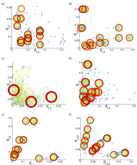
Empirically, we have found very interesting and remarkable cyclic dynamics in many differ-ent low-dimensional cases (many more cases than the ones analyzed in this paper), for example, those illustrated in Figure 6. In fact, we have empirically found that AdaBoost produces cycles on randomly generated matrices – even on random matrices with hundreds of dimensions. On low-dimensional random matrices, cycles are almost always produced in our experiments. Thus, the story of AdaBoost’s dynamics does not end with the margins; it is important to study AdaBoost’s dynamics in more general cases where these cycles occur in order to understand its convergence properties.

To this extent, we prove that if AdaBoost cycles, it cycles only among a set of “support vec-tors” that achieve the same smallest margin among training examples. In this sense, we confirm observations of Caprile et al. (2002) who previously studied the dynamical behavior of boosting, and who also identified two sorts of examples which they termed “easy” and “hard.” In addition, we give sufficient conditions for AdaBoost to achieve a maximum margin solution when cycling occurs. We also show that AdaBoost treats identically classified examples as one example, in the sense we will describe in Section 6. In Section 10, we discuss a case in which AdaBoost exhibits indications of chaotic behavior, namely sensitivity to initial conditions, and movement into and out of cyclic behavior.

2. Notation and Introduction to AdaBoost

The training set consists of examples with labels_{(xi,yi)}i=1,...,m, where(xi,yi)∈

X

X

H

weak classifiers that can be produced by the weak learning algorithm, where hj :

X

H

H

and since we restrict our attention to their behavior on a finite training set, we can assume the number of weak classifiers n is finite. We typically think of n as being very large, mn, which makes a gradient descent calculation impractical because n, the number of dimensions, is too large; hence, AdaBoost uses coordinate descent instead, where only one weak classifier is chosen at each iteration.

We define an m×n matrix M where Mi j =yihj(xi), i.e., Mi j = +1 if training example i is classified correctly by weak classifier hj, and₋1 otherwise. We assume that no column of M has all +1’s, that is, no weak classifier can classify all the training examples correctly. (Otherwise the learning problem is trivial. In this case, AdaBoost will have an undefined step size.) Although

M is too large to be explicitly constructed in practice, mathematically, it acts as the only “input”

to AdaBoost in this notation, containing all the necessary information about the weak learning algorithm and training examples.

AdaBoost computes a set of coefficients over the weak classifiers. At iteration t, the (unnor-malized) coefficient vector is denotedλt; i.e., the coefficient of weak classifier hj determined by AdaBoost at iteration t isλt,j. The final combined classifier that AdaBoost outputs is fλ_tmax given

viaλtmax/kλtmaxk1:

fλ=

∑n

j=1λjhj

kλ_k1

where _kλ_k1= n

∑

|λj|.

In the specific examples we provide, either hjor−hjremains unused over the course of AdaBoost’s iterations, so all values of λt,j are non-negative. The margin of training example i is defined by yifλ(x_i). Informally, one can think of the margin of a training example as the distance (by some

measure) from the example to the decision boundary,_{x : fλ(x) =0}.

A boosting algorithm maintains a distribution, or set of weights, over the training examples that is updated at each iteration t. This distribution is denoted dt _∈∆m, and dT_t is its transpose. Here,

∆mdenotes the simplex of m-dimensional vectors with non-negative entries that sum to 1. At each iteration t, a weak classifier hjt is selected by the weak learning algorithm. The probability of error

at iteration t, denoted d₋, for the selected weak classifier hjt on the training examples (weighted by dt) is∑_{i:M_{i jt}=−1_}dt,i. Also, denote d+:=1−d−. Note that d+and d− depend on t; although we

have simplified the notation, the iteration number will be clear from the context. The edge of weak classifier jt at time t with respect to the training examples is(dT_t M)jt, which can be written as

(d_tTM)jt =

∑

i:Mi jt=1

dt,i−

∑

dt,i=d+−d−=1−2d−.

Thus, a smaller edge indicates a higher probability of error. For the optimal case (the case we usually consider), we will require the weak learning algorithm to give us the weak classifier with the largest possible edge at each iteration,

jt ∈ argmax j

i.e., jt is the weak classifier that performs the best on the training examples weighted by dt. For the non-optimal case (which we consider in Section 8), we only require a weak classifier whose edge exceedsρ, whereρis the largest possible margin that can be attained for M, i.e.,

jt ∈ {j :(dTt M)j≥ρ}.

(The valueρis defined formally below.) The edge for the chosen weak classifier jt at iteration t is denoted rt, i.e., rt = (d_tTM)jt. Note that d+= (1+rt)/2 and d−= (1−rt)/2.

The margin theory developed via a set of generalization bounds that are based on the margin dis-tribution of the training examples (Schapire et al., 1998; Koltchinskii and Panchenko, 2002). These bounds can be reformulated (in a slightly weaker form) in terms of the minimum margin, which was the focus of previous work by Breiman (1999), Grove and Schuurmans (1998), and R¨atsch and War-muth (2002). Thus, these bounds suggest maximizing the minimum margin over training examples to achieve a low probability of error over test data. Hence, our goal is to find a normalized vector

˜

λ_∈∆n that maximizes the minimum margin over training examples, mini (M ˜λ)i (or equivalently miniyifλ(x_i)). That is, we wish to find a vector

˜

λ_∈ argmax ¯

λ_∈∆_n

min i (M ¯λ)i.

We call this minimum margin over training examples (i.e., mini(Mλ)i/kλk1) the`1-margin or sim-ply margin of classifierλ. Any training example that achieves this minimum margin will be called a support vector. Due to the von Neumann Min-Max Theorem for 2-player zero-sum games,

min d∈∆m

max j (d

T_M)

j=max ˜

λ_∈∆_n

min i (M ˜λ)i.

That is, the minimum value of the edge (left hand side) corresponds to the maximum value of the margin (i.e., the maximum value of the minimum margin over training examples, right hand side). We denote this value by ρ. One can think ofρ as measuring the worst performance of the best combined classifier, mini(M ˜λ)i.

The “unrealizable” or “non-separable” case where ρ=0 is fully understood (Collins et al., 2002). For this work, we assumeρ>0 and study the less understood “realizeable” or “separable” case. In both the non-separable and separable cases, AdaBoost converges to a minimizer of the empirical loss function

F(λ):= m

∑

e−(Mλ)i_.

In the non-separable case, the dt’s converge to a fixed vector (Collins et al., 2002). In the separable case, the dt’s cannot converge to a fixed vector, and the minimum value of F is 0, occurring as_||λ_||1→∞. It is important to appreciate that this tells us nothing about the value of the margin achieved by AdaBoost or any other procedure designed to minimize F. To see why, consider any

¯

AdaBoost (“optimal” case):

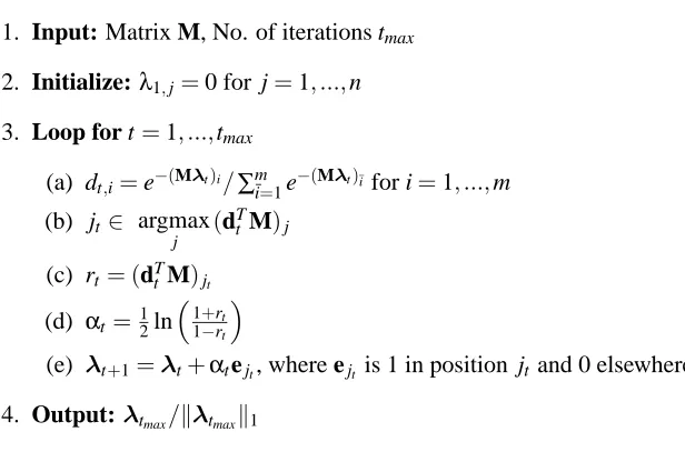
1. Input: Matrix M, No. of iterations tmax 2. Initialize:λ1,j=0 for j=1, ...,n 3. Loop for t=1, ...,tmax

(a) dt,i=e−(M

λ_t)i /∑m

¯i=1e−( Mλ_t)

i for i=1, ...,m

(b) jt_∈ argmax j (d

T t M)j (c) rt= (dT_t M)jt

(d) αt= 1₂ln

1+rt

1−rt

(e) λt+1=λt+αtejt, where ejt is 1 in position jt and 0 elsewhere.

4. Output:λtmax/kλtmaxk1

Figure 1: Pseudocode for the AdaBoost algorithm.

of coordinate descent that awards AdaBoost its ability to increase margins, not simply AdaBoost’s ability to minimize F. The value of the function F tells us very little about the value of the margin; even asymptotically, it only tells us whether the margin is positive or not.

Figure 1 shows pseudocode for the AdaBoost algorithm. Usually theλ1vector is initialized to zero, so that all the training examples are weighted equally during the first iteration. The weight vector dt is adjusted so that training examples that were misclassified at the previous iteration are weighted more highly, so they are more likely to be correctly classified at the next iteration. The weight vector dt is determined from the vector of coefficientsλt, which has been updated. The map from dt to dt+1 also involves renormalization, so it is not a very direct map when written in this form. Thus on each round of boosting, the distribution dt is updated and renormalized (Step 3a), classifier jt with maximum edge (minimum probability of error) is selected (Step 3b), and the weight of that classifier is updated (Step 3e). Note thatλt,j=∑t_˜t=1α˜t1j˜t=j where 1j˜t=jis 1 if j˜t= j

and 0 otherwise.

3. The Iterated Map Defined By AdaBoost

AdaBoost can be reduced to an iterated map for the dt’s, as shown in Figure 2. This map gives a direct relationship between dt and dt+1, taking the normalization of Step 3a into account

automat-ically. For the cases considered in Sections 4, 5, and 6, we only need to understand the dynamics of Figure 2 in order to compute the final coefficient vector that AdaBoost will output. Initialize d1,i =1/m for i=1, ...,m as in the first iteration of AdaBoost. Also recall that all values of rt are nonnegative since rt_≥ρ>0.

To show the equivalence with AdaBoost, consider the iteration defined by AdaBoost and reduce as follows. Since:

αt =

1 2ln

1+rt 1₋rt

, we have e−(Mi jtαt)₌

1₋rt 1+rt

1 2Mi jt

=

1₋Mi jtrt

1+Mi jtrt

Iterated Map Defined by AdaBoost 1. jt_∈ argmax

j (d T t M)j

2. rt= (dT_t M)jt

3. dt+1,i=₁₊d_Mt,i

i jtrt for i=1, ...,m

Figure 2: The nonlinear iterated map obeyed by AdaBoost’s weight vectors. This dynamical system provides a direct map from dt to dt+1.

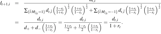
Here, we have used the fact that M is a binary matrix. The iteration defined by AdaBoost combined with the equation above yields:

dt+1,i =

e−(Mλt)i_e−(Mi jtαt)

∑m

¯i=1e−(M

λ_t)

¯i_e−(M¯ijtαt) =

dt,i

∑m

¯i=1dt,¯i

_1−M

¯ijtrt

1+M_¯ijtrt

1 2_1+M

i jtrt

1−M_{i jt}rt

1 2 .

Here, we have divided numerator and denominator by∑m_˜i=1e−(Mλ_t)

˜i_{. For each i such that Mi j} t =1,

we find:

dt+1,i =

dt,i

∑_{¯i:M_¯ijt=1}dt,¯i

1−rt

1+rt

1 2_1+r

t

1−rt

1 2

+∑_{¯i:M_¯ijt=−1}dt,¯i

1+rt

1−rt

1 2_1+r

t

1−rt

1 2

= dt,i

d++d−

1+rt

1−rt

= dt,i 1+rt

2 + 1−rt

2

1+rt

1−rt

= dt,i 1+rt

.

Likewise, for each i such that Mi jt =−1, we find dt+1,i=

dt,i

1−rt. Thus our reduction is complete. To

check that∑m_i=1dt+1,i=1, i.e., that renormalization has been taken into account by the iterated map, we calculate:

m

∑

dt+1,i= 1 1+rt

d++

1 1₋rt

d₋= (1+rt) 2(1+rt)

+ (1−rt) 2(1₋rt)

=1.

For the iterated map, fixed points (rather than cycles or other dynamics) occur when the training data fails to be separable by the set of weak classifiers. In that case, the analysis of Collins, Schapire, and Singer (2002) shows that the iterated map will converge to a fixed point, and that theλ0_ts will asymptotically attain the minimum value of the convex function F(λ):=∑m

i=1e−(M

λ_)i

, which is strictly positive in the non-separable case. Consider the possibility of fixed points for the dt’s in the separable caseρ>0. From our dynamics, we can see that this is not possible, since rt _≥ρ>0 and for any i such that dt,i>0,

dt+1,i=

dt,i (1+Mi,jtrt)

6

=dt,i.

4. The Dynamics of AdaBoost in the Simplest Case : The 3_×3 Case

In this section, we will introduce a simple 3_×3 input matrix (in fact, the simplest non-trivial matrix) and analyze the convergence of AdaBoost in this case, using the iterated map of Section 3. We will show that AdaBoost does produce a maximum margin solution, remarkably through convergence to one of two stable limit cycles. We extend this example to the m_×m case in Section 5, where AdaBoost produces at least(m₋1)! stable limit cycles, each corresponding to a maximum margin solution. We will also extend this example in Section 6 to include manifolds of cycles.

Consider the input matrix

M=

  −

1 1 1 1 ₋1 1 1 1 −1

 

corresponding to the case where each classifier misclassifies one of three training examples. We could add columns to include the negated version of each weak classifier, but those columns would never be chosen by AdaBoost, so they have been removed for simplicity. The value of the margin for the best combined classifier defined by M is 1/3. How will AdaBoost achieve this result? We will proceed step by step.

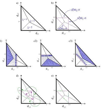
Assume we are in the optimal case, where jt∈argmaxj(dTt M)j. Consider the dynamical system on the simplex∆3 defined by our iterated map in Section 3. In the triangular region with vertices (0,0,1),(1₃,1₃,1₃),(0,1,0), jt will be 1 for Step 1 of the iterated map. That is, within this region, dt,1<dt,2and dt,1<dt,3, so jt will be 1. Similarly, we have regions for jt=2 and jt =3 (see Figure 3(a)).

AdaBoost was designed to set the edge of the previous weak classifier to 0 at each iteration, that is, dt+1will always satisfy(dtT+1M)jt =0. To see this using the iterated map,

(dT_t+1M)jt =

∑

{i:M_{i jt}=1}

dt,i 1

1+rt −_{i:M

∑

i jt=−1}

dt,i 1 1₋rt = d+

1 1+rt −

d₋ 1 1₋rt

=1+rt 2

1 1+rt −

1₋rt 2

1 1₋rt

=0. (1)

This implies that after the first iteration, the dt’s are restricted to

{d :[(dTM)1=0] [

[(dTM)2=0] [

[(dTM)3=0]}.

Thus, it is sufficient for our dynamical system to be analyzed on the edges of a triangle with vertices 0,1

2, 1 2

, 1₂,0,1 2

, 1₂,1 2,0

(see Figure 3(b)). That is, within one iteration, the 2-dimensional map on the simplex∆3reduces to a 1-dimensional map on the edges of the triangle.

Consider the possibility of periodic cycles for the dt’s. If there are periodic cycles of length T , then the following condition must hold for dcyc₁ , ...,dcyc_T in the cycle: For each i, either

• d₁cyc_,i =0,or

• ∏Tt=1(1+Mi jtr

cyc t ) =1,

where rcyc_t = (dcycT_t M)jt. (As usual, d

cyc t

T

a) b)

t,2

t,1

j = 1

j = 2_t

t _{j = 3}

t 1 1 d d 1/3 1/3 t,1 t,2

(d M) =0

(d M) =0

(d M) =0

2 1 3 t t t T T T 1 1 1/2 d d 1/2

c1) c2) c3)

t,1 t,2 1 1 1/2 d 1/2 d t,1 t,2 !!!!!!!!! !!!!!!!!! !!!!!!!!! !!!!!!!!! !!!!!!!!! !!!!!!!!! !!!!!!!!! !!!!!!!!! !!!!!!!!! !!!!!!!!! !!!!!!!!! !!!!!!!!!

""""""""""""""

### ### ### ### ### ### ### ### ### ### ### $$ $$ $$ $$ $$ $$ $$ $$ $$ $$ $$ %%% %%% %%% %%% %%% %%% %%% %%% %%% %%%

&&& &&& &&& &&& &&& &&& &&& &&& &&& &&&

''''' ''''' ''''' ''''' ''''' ''''' ''''' ''''' ''''' ''''' ((((( ((((( ((((( ((((( ((((( ((((( ((((( ((((( ((((( ((((( ))))))) ))))))) ))))))) ))))))) ))))))) ))))))) ))))))) ))))))) ))))))) ))))))) ))))))) ))))))) ******* ******* ******* ******* ******* ******* ******* ******* ******* ******* ******* ******* +++++++ +++++++ +++++++ +++++++ +++++++ +++++++ +++++++ +++++++ +++++++ +++++++ ,,,,,,, ,,,,,,, ,,,,,,, ,,,,,,, ,,,,,,, ,,,,,,, ,,,,,,, ,,,,,,, ,,,,,,, ,,,,,,, --- ---- ---- ---- ---- ---- ---- ---- ---- ---- ---- -.... .... .... .... .... .... .... .... .... .... .... / / / / / / / / / / / / 0 0 0 0 0 0 0 0 0 0 0 0 1 1 1/2 d 1/2 d t,1 t,2

1111111111111111111111111 1111111111111111111111111 1111111111111111111111111 1111111111111111111111111 1111111111111111111111111 1111111111111111111111111 1111111111111111111111111 1111111111111111111111111 1111111111111111111111111 1111111111111111111111111 1111111111111111111111111 1111111111111111111111111 1111111111111111111111111 1111111111111111111111111 1111111111111111111111111 1111111111111111111111111 1111111111111111111111111 1111111111111111111111111 1111111111111111111111111 1111111111111111111111111 1111111111111111111111111 1111111111111111111111111 1111111111111111111111111 1111111111111111111111111 1111111111111111111111111

2222222222222222222222222 2222222222222222222222222 2222222222222222222222222 2222222222222222222222222 2222222222222222222222222 2222222222222222222222222 2222222222222222222222222 2222222222222222222222222 2222222222222222222222222 2222222222222222222222222 2222222222222222222222222 2222222222222222222222222 2222222222222222222222222 2222222222222222222222222 2222222222222222222222222 2222222222222222222222222 2222222222222222222222222 2222222222222222222222222 2222222222222222222222222 2222222222222222222222222 2222222222222222222222222 2222222222222222222222222 2222222222222222222222222 2222222222222222222222222 2222222222222222222222222

33 33 33 33 33 33 33 33 33 33 33 4 4 4 4 4 4 4 4 4 4 4 55 55 55 55 55 55 55 55 55 66 66 66 66 66 66 66 66

777 777 777 777 777 777 777 777

888 888 888 888 888 888 888 888

999 999 999 999 999 999

::: ::: ::: ::: ::: ::: ;;;;; ;;;;; ;;;;; ;;;;; ;;;;; ;;;;; ;;;;;

<<<<< <<<<< <<<<< <<<<< <<<<< <<<<< <<<<<

===== ===== ===== ===== ===== =====

>>>>> >>>>> >>>>> >>>>> >>>>> >>>>>

???? ???? ???? ???? @@@@ @@@@ @@@@ @@@@

AAAAAA AAAAAA AAAAAA AAAAAA AAAAAA

BBBBBB BBBBBB BBBBBB BBBBBB BBBBBB

CCCCCCC CCCCCCC CCCCCCC

DDDDDDD DDDDDDD DDDDDDD

EEEEEEEEEEE

FFFFFFFFFFF

GGGGGGGGGG GGGGGGGGGG GGGGGGGGGG

HHHHHHHHHH HHHHHHHHHH HHHHHHHHHH 1 1 1/2 d 1/2 d d) e) t,1 t,2 1 1 1/2 d 1/2 d t,1 t,2 x x x 1 1 1/2 d 1/2 d

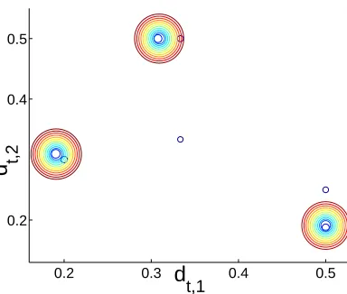
Figure 3: (a) Regions of dt-space where classifiers jt=1,2,3 will respectively be selected for Step 1 of the iterated map of Figure 2. Since dt,3 =1−dt,2−dt,1, this projection onto the first two coordinates dt,1 and dt,2 completely characterizes the map. (b) Regardless of the initial position d1, the weight vectors at all subsequent iterations d2, ...,dtmax will be

0.2 0.3 0.4 0.5 0.2

0.4 0.5

d

d

Figure 4: 50 iterations of AdaBoost showing convergence of dt’s to a cycle. Small rings indicate earlier iterations of AdaBoost, while larger rings indicate later iterations. There are many concentric rings at positions dcyc₁ , dcyc₂ , and dcyc₃ .

Consider the possibility of a periodic cycle of length 3, cycling through each weak classifier once. For now, assume j1=1,j2=2,j3=3, but without loss of generality one can choose j1= 1,j2=3,j3=2, which yields another cycle. Assume d1cyc,i >0 for all i. From the cycle condition,

1 = (1+Mi j1r

cyc

1 )(1+Mi j2r

cyc

2 )(1+Mi j3r

cyc

3 ) for i=1,2,and 3, i.e.,

1 = (1₋r₁cyc)(1+r₂cyc)(1+r₃cyc) for i=1, (2) 1 = (1+r₁cyc)(1₋r₂cyc)(1+r₃cyc) for i=2, (3) 1 = (1+r₁cyc)(1+r₂cyc)(1₋r₃cyc) for i=3. (4) From (2) and (3),

(1₋rcyc₁ )(1+r₂cyc) = (1+rcyc₁ )(1₋r₂cyc),

thus r₁cyc=rcyc₂ . Similarly, rcyc₂ =r₃cyc from (3) and (4), so r₁cyc=rcyc₂ =rcyc₃ . Using either (2), (3), or (4) to solve for r :=r₁cyc=rcyc₂ =rcyc₃ (taking positive roots since r>0), we find the value of the edge for every iteration in the cycle to be equal to the golden ratio minus one, i.e.,

r=

√

5₋1 2 .

Now, let us solve for the weight vectors in the cycle, dcyc₁ , dcyc₂ , and dcyc₃ . At t =2, the edge with respect to classifier 1 is 0. Again, it is required that each dcyct lies on the simplex∆3.

(dcyc₂ TM)1=0 and 3

∑

dcyc_2,i =1, that is,

−d₂cyc_,1+d₂cyc_,2+d₂cyc_,3 =0 and d₂cyc_,1+d₂cyc_,2+d₂cyc_,3 =1,

Since d₂cyc_,1 =1

2, we have d cyc

2,2 = 12−d cyc

2,3. At t=3, the edge with respect to classifier 2 is 0. From the iterated map, we can write dcyc₃ in terms of dcyc₂ .

0= (dcyc₃ TM)2= 3

∑

Mi2d₂cyc_,i 1+Mi2r =

1 2 1+r−

1 2−d

cyc 2,3 1₋r +

d₂cyc_,3 1+r, so

d₂cyc_,3 =r 2=

√

5₋1

4 and thus d cyc 2,2 =

1 2−d

cyc 2,3 =

3₋√5 4 . Now that we have found dcyc₂ , we can recover the rest of the cycle:

dcyc₁ = 3−

√

5 4 ,

√

5₋1 4 ,

1 2

!T

,

dcyc₂ = 1 2,

3₋√5 4 ,

√

5₋1 4

!T

,

dcyc₃ =

√

5₋1 4 ,

1 2,

3₋√5 4

!T

.

To check that this actually is a cycle, starting from dcyc₁ , AdaBoost will choose jt =1. Then r1= (dcyc₁ TM)1=

√

5−1

2 . Now, computing dcyc_1,i

1+Mi,1r1 for all i yields d

cyc

2 . In this way, AdaBoost will cycle between weak classifiers j=1,2,3,1,2,3,etc.

The other 3-cycle can be determined similarly:

dcyc₁ 0 = 3−

√

5 4 ,

1 2,

√

5₋1 4

!T

,

dcyc₂ 0 = 1 2,

√

5₋1 4 ,

3₋√5 4

!T

,

dcyc₃ 0 =

√

5₋1 4 ,

3₋√5 4 ,

1 2

!T

.

Since we always start from the initial condition d1= 1₃,1₃,1₃

T

, the initial choice of jt is arbitrary; all three weak classifiers are within the argmax set in Step 1 of the iterated map. This arbitrary step, along with another arbitrary choice at the second iteration, determines which of the two cycles the algorithm will choose; as we will see, the algorithm must converge to one of these two cycles.

converge to these points. For the first endpoint the map is not defined, and for the second, the map is ambiguous; not well-defined.) For this subregion jt =1, and the next iterate is

x 1₋(1₋2x),

1 2 1+ (1₋2x),

1 2−x 1+ (1₋2x)

!T =

1 2,

1 4(1₋x),

1 2−

1 4(1₋x)

T

.

To compare the length of the new interval with the length of the previous interval, we use the fact that there is only one degree of freedom. A position on the previous interval can be uniquely determined by its first component x_∈(0,1₄). A position on the new interval can be uniquely determined by its second component taking values ₄₍₁1_−x), where we still have x_∈(0,1

4). The map x_7→ 1

4(1₋x) is a contraction. To see this, the slope of the map is ₄₍₁1

−x)2, taking values within the interval(1₄,4₉).

Thus the map is continuous and monotonic, with absolute slope strictly less than 1. The next it-erate will appear within the interval 1₂,1₄,1₄T to 1₂,1₃,1₆T, which is strictly contained within the subregion connecting 1₂,1₄,1₄T with 1₂,1₂,0T. Thus, we have a contraction. A similar calculation can be performed for each of the subregions, showing that each subregion maps monotonically to an area strictly within another subregion by a contraction map. Figure 3(d) illustrates the various mappings between subregions. After three iterations, each subregion maps by a monotonic con-traction to a strict subset of itself. Thus, any fixed point of the three-iteration cycle must be the unique attracting fixed point for that subregion, and the domain of attraction for this point must be the whole subregion. In fact, there are six such fixed points, one for each subregion, three for each of the two cycles. The union of the domains of attraction for these fixed points is the whole triangle; every position d within the simplex∆3 is within the domain of attraction of one of these 3-cycles. Thus, these two cycles are globally stable.

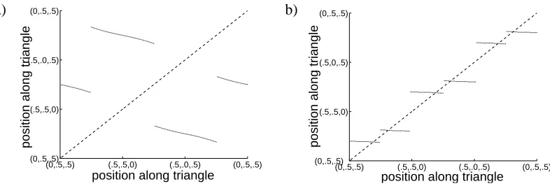
Since the contraction is so strong at every iteration (as shown above, the absolute slope of the map is much less than 1), the convergence to one of these two 3-cycles is very fast. Figure 5(a) shows where each subregion of the “unfolded triangle” will map after the first iteration. The “unfolded triangle” is the interval obtained by traversing the triangle clockwise, starting and ending at 0,1₂,1₂. Figure 5(b) illustrates that the absolute slope of the second iteration of this map at the fixed points is much less than 1; the cycles are strongly attracting.

The combined classifier that AdaBoost will output is

λcombined=

1 2ln

₁

+rcyc₁ 1−rcyc₁

,1 2ln

₁

+rcyc₂ 1−rcyc₂

,1 2ln

_1+rcyc 3

1−rcyc₃

T

normalization constant =

1 3,

1 3,

1 3

T

,

and since mini(Mλcombined)i=1₃, we see that AdaBoost always produces a maximum margin solu-tion for this input matrix.

Thus, we have derived our first convergence proof for AdaBoost in a specific separable case. We have shown that at least in some cases, AdaBoost is in fact a margin-maximizing algorithm. We summarize this first main result.

a) b)

(0,.5,.5) (.5,.5,0) (.5,.0,.5) (0,.5,.5)

(0,.5,.5) (.5,.5,0) (.5,.0,.5) (0,.5,.5)

position along triangle

position along triangle

(0,.5,.5) (.5,.5,0) (.5,.0,.5) (0,.5,.5)

(0,.5,.5) (.5,.5,0) (.5,0,.5) (0,.5,.5)

position along triangle

position along triangle

Figure 5: (a) The iterated map on the unfolded triangle. Both axes give coordinates on the edges of the inner triangle in Figure 3(b). The plot shows where dt+1 will be, given dt. (b) The map from (a) iterated twice, showing where dt+3will be, given dt. For this “triple map”, there are 6 stable fixed points, 3 for each cycle.

• The weight vectors dt converge to one of two possible stable cycles. The coordinates of the cycles are:

dcyc₁ = 3−

√

5 4 ,

√

5₋1 4 ,

1 2

!T

,

dcyc₂ = 1 2,

3₋√5 4 ,

√

5₋1 4

!T

,

dcyc₃ =

√

5₋1 4 ,

1 2,

3₋√5 4

!T

,

and

dcyc₁ 0 = 3−

√

5 4 ,

1 2,

√

5₋1 4

!T

,

dcyc₂ 0 = 1 2,

√

5₋1 4 ,

3₋√5 4

!T

,

dcyc₃ 0 =

√

5₋1 4 ,

3₋√5 4 ,

1 2

!T

.

• AdaBoost produces a maximum margin solution for this matrix M.

5. Generalization to m Classifiers, Each with One Misclassified Example

where there is a rotation of the coordinates at every iteration and a contraction. Here,

M=

       

−1 1 1 _··· 1

1 ₋1 1 _··· 1 1 1 ₋1 ...

..

. . .. 1

1 _{··· ···} 1 ₋1

       

.

Theorem 2 For the m_×m matrix above:

• The dynamical system for AdaBoost’s weight vectors contains at least(m₋1)! stable periodic cycles of length m.

• AdaBoost converges to a maximum margin solution when the weight vectors converge to one of these cycles.

The proof of Theorem 2 can be found in Appendix A.

6. Identically Classified Examples and Manifolds of Cycles

In this section, we show how manifolds of cycles appear automatically from cyclic dynamics when there are sets of identically classified training examples. We show that the manifolds of cycles that arise from a variation of the 3_×3 case are stable. One should think of a “manifold of cycles” as a continuum of cycles; starting from a position on any cycle, if we move along the directions defined by the manifold, we will find starting positions for infinitely many other cycles. These manifolds are interesting from a theoretical viewpoint. In addition, their existence and stability will be an essential part of the proof of Theorem 7.

A set of training examples

I

contained in

I

For convenience of notation, we will remove the ‘cyc’ notation so that d1is a position within the cycle (or equivalently, we could make the assumption that AdaBoost starts on a cycle). Say there exists a cycle such that d1,i>0∀i∈

I

I

I

with i_∈

I

I

Mi jt =Mi0jt ∀t=1, ...,T . Let perturbation a∈R

m_obey

∑

¯i_∈I

a¯i=0, and also ai=0 for i∈/

I

must still be a valid distribution, so it must obey the constraint da₁∈∆m, i.e.,∑iai=0 as we have specified. Choose any elements i and i0_∈

I

ra₁ = (da₁TM)j1= (d1

T_M) j1+ (a

T_M)

j1 =r1+

∑

¯i∈I

a¯iM¯ij1=r1+Mi0j1

∑

¯i∈I

a¯i=r1

d₂a_,i = d a 1,i 1+Mi j1r

a 1

= d

a 1,i 1+Mi j1r1

= d1,i 1+Mi j1r1

+ 1

1+Mi0_j1r₁ai=d2,i+ 1 1+Mi0_j1r₁ai ra₂ = (da₂TM)j2= (d2

T_M) j2+

1 1+Mi0_j1r1(a

T_M)

j2=r2+

1

1+Mi0_j1r1

∑

a_¯iM_¯ij2

= r2+ Mi0j2

1+Mi0_j1r1

∑

∈I

a¯i=r2

d₂a_,i = d a 2,i 1+Mi j2r

a 2

= d

a 2,i 1+Mi j2r2

= d2,i 1+Mi j2r2

+ 1

(1+Mi0_j2r2)(1+M_i0_j1r1)ai

= d3,i+

1

(1+Mi0_j2r₂)(1+M_i0_j1r₁)ai ..

.

d_Ta_+1,i = dT+1,i+

1

∏T

t=1(1+Mi0jtrt)

ai=d1,i+ai=d1a,i.

The cycle condition was used in the last line. This calculation shows that if we perturb any cycle in the directions defined by

I

corresponding to the possible nonzero acceptable perturbations a. Effectively, the perturbation shifts the distribution among examples in

I

a cycle exists containing vector d1with d1,1=.20,d1,2=.10, and d1,3=.30, where{1,2,3} ⊂

I

We will now consider a simple case where manifolds of cycles exist, and we will show that these manifolds are stable in the proof of Theorem 3.

The form of the matrix M is _                       

−1 1 1 ..

. ... ...

−1 1 1

1 ₋1 1

..

. ... ...

1 ₋1 1

1 1 ₋1

..

. ... ...

1 1 ₋1

1 1 1

..

. ... ...

1 1 1

                        .

examples are always correctly classified (their weights converge to zero). Thus we consider the components of d as belonging to one of four pieces; as long as

q1

∑

di,

q1+q2

∑

di,

q1+q2+q3

∑

di

!T

=dcyc₁ ,dcyc₂ ,dcyc₃ ,dcyc₁ 0,dcyc₂ 0, or dcyc₃ 0from Section 4,

then d lies on a 3-cycle as we have just shown.

Theorem 3 For the matrix M defined above, manifolds of cycles exist (there is a continuum of

cycles). These manifolds are stable.

The proof of Theorem 3 can be found in Appendix B.

7. Cycles and Support Vectors

Our goal is to understand general properties of AdaBoost in cases where cycling occurs, to broaden our understanding of the phenomenon we have observed in Sections 4, 5, and 6. Specifically, we show that if cyclic dynamics occur, the training examples with the smallest margin are the training examples whose dt,i values stay non-zero (the “support vectors”). In the process, we provide a formula that allows us to directly calculate AdaBoost’s asymptotic margin from the edges at each iteration of the cycle. Finally, we give sufficient conditions for AdaBoost to produce a maximum margin solution when cycling occurs.

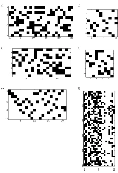
As demonstrated in Figure 6, there are many low-dimensional matrices M for which AdaBoost empirically produces cyclic behavior. The matrices used to generate the cycle plots in Figure 6 are contained in Figure 7. These matrices were generated randomly and reduced (rows and columns that did not seem to play a role in the asymptotic behavior were eliminated). We observe cyclic behavior in many more cases than are shown in the figure; almost every low-dimensional random matrix that we tried (and even some larger matrices) seems to yield cyclic behavior. Our empirical observations of cyclic behavior in many cases leads us to build an understanding of AdaBoost’s general asymptotic behavior in cases where cycles exist, though there is not necessarily a contraction at each iteration so the dynamics may be harder to analyze. (We at least assume the cycles AdaBoost produces are stable, since it is not likely we would observe them otherwise.) These cyclic dynamics may not persist in very large experimental cases, but from our empirical evidence, it seems plausible (even likely) that cyclic behavior might persist in cases in which there are very few support vectors.

When AdaBoost converges to a cycle, it “chooses” a set of rows and a set of columns, that is:

• The jt’s cycle amongst some of the columns of M, but not necessarily all of the columns. In order for AdaBoost to produce a maximum margin solution, it must choose a set of columns such that the maximum margin for M can be attained using only those columns.

• The values of dt,i(for a fixed value of i) are either always 0 or always strictly positive through-out the cycle. A support vector is a training example i such that the dt,i’s in the cycle are

a) b)

0 0.1 0.2 0.3

0 0.1 0.25 0.35

d t,1

d t,2

0 0.1 0.3 0.4 0.5

0 0.05 0.15 0.2 0.25

d t,1

d t,2

c) d)

0 0.05 0.15 0.25

0 0.05 0.25 0.35

d t,1

d t,2

0 0.1 0.2 0.3

0 0.1 0.3 0.4

d t,1

d t,2

e) f)

0 0.1 0.35 0.45

0 0.1 0.4 0.5

d t,1

d t,2

0 0.05 0.15 0.2

0 0.05 0.15 0.2

d t,11

d t,12

a) b)

1 5 10 15 20 25

1

4

8

12

2 4 6 8 10

2

4

6

8

10

c) d)

5 10 15

2

4

6

8

10

2 4 6 8

2

4

6

8

10

e) f)

5 10 15 20

1

5

8

11

1

10

20

1

10

20

30

40

50

for the algorithm to classify, since they have margin larger than the support vectors. For sup-port vectors, the cycle condition holds,∏T_t=1(1+Mi jtr

cyc

t ) =1. (This holds by Step 3 of the iterated map.) For non-support vectors,∏_tT₌₁(1+Mi jtr

cyc

t )>1 so the dt,i’s converge to 0 (the cycle must be stable).

Theorem 4 AdaBoost produces the same margin for each support vector and larger margins for

other training examples. This margin can be expressed in terms of the cycle parameters r₁cyc, ...,rcyc_T .

Proof Assume AdaBoost is cycling. Assume d1is within the cycle for ease of notation. The cycle produces a normalized outputλcyc:=limt→∞λt/||λt||1for AdaBoost. (This limit always converges when AdaBoost converges to a cycle.) Denote

zcyc:= T

∑

αt =

T

∑

1 2ln

1+rt 1₋rt

.

Let i be a support vector. Then,

(Mλcyc)i = 1 zcyc

T

∑

Mi jtαt=

1 zcyc

T

∑

Mi jt

1 2ln

1+rt 1₋rt

= 1

2zcyc T

∑

ln

1+Mi jtrt

1₋Mi jtrt

= 1 2zcycln " T

∏

1+Mi jtrt

1₋Mi jtrt

#

= 1

2zcycln





∏

t=1

1+Mi jtrt

1₋Mi jtrt

!

T

∏

1 (1+Mi jtrt)

!2

 = 1 2zcycln " T

∏

1

(1₋Mi jtrt)(1+Mi jtrt)

# = 1 2zcycln " T

∏

1 1₋rt2

#

=₋1 2

ln∏_tT₌₁(1₋r_t2)

∑T

et=1 1 2ln

₁

+r_et 1₋r_et

= ₋ln∏ T

t=1(1−rt2) ln∏_eT_t=1

_1+r

e

t

1₋r_et

. (5)

The first line uses the definition ofαt from the AdaBoost algorithm, the second line uses the fact that M is binary, the third line uses the fact that i is a support vector, i.e., ∏_tT₌₁(1+Mi jtrt) =1.

Since the value in (5) is independent of i, this is the value of the margin that AdaBoost assigns to every support vector i. We denote the value in (5) as µcycle, which is only a function of the cycle parameters, i.e., the edge values.

Now we show that every support vector achieves a larger margin than µcycle. For a non-support vector i, we have∏T_t=1(1+Mi jtrt)>1, that is, the cycle is stable. Thus, 0>ln

h

1

∏T

t=1(1+Mi jtrt)

Now,

(Mλcyc)i = 1 zcyc

T

∑

Mi jtαt=

1 2zcycln

_∏

t(1+Mi jtrt)

∏˜t(1−Mi j˜tr˜t)

> 1

2zcyc ln

_∏

t(1+Mi jtrt)

∏˜t(1−Mi j˜tr˜t)

+ 1

2zcyc ln

1

∏˜t(1+Mi j˜tr˜t)

2

= −ln∏ T

t=1(1−r2t) ln∏T_et=11+ret

1−r_et

=µcycle.

Thus, non-support vectors achieve larger margins than support vectors.

The previous theorem shows that the asymptotic margin of the support vectors is the same as the asymptotic margin produced by AdaBoost; this asymptotic margin can be directly computed using (5). AdaBoost may not always produce a maximum margin solution, as we will see in Sections 8 and 9; however, there are sufficient conditions such that AdaBoost will automatically produce a maximum margin solution when cycling occurs. Before we state these conditions, we define the matrix Mcyc_{∈ {−}1,1_}mcyc×ncyc_{, which contains certain rows and columns of M. To construct Mcyc}

from M, we choose only the rows of M that correspond to support vectors (eliminating the others, whose weights vanish anyway), and choose only the columns of M corresponding to weak classifiers that are chosen in the cycle (eliminating the others, which are never chosen after cycling begins anyway). Here, mcycis the number of support vectors chosen by AdaBoost, and ncycis the number of weak classifiers in the cycle.

Theorem 5 Suppose AdaBoost is cycling, and that the following are true:

1.

max ˆ

λ_∈∆_ncyc

min i (Mcyc

ˆ

λ)i=max ˜

λ_∈∆_n

min

i (M ˜λ)i=ρ

(AdaBoost cycles among columns of M that can be used to produce a maximum margin solu-tion.)

2. There existsλ_ρ∈∆ncycsuch that(Mcycλρ)i=ρfor i=1, ...,mcyc. (AdaBoost chooses support

vectors corresponding to a maximum margin solution for Mcyc.)

3. The matrix Mcycis invertible.

Then AdaBoost produces a maximum margin solution.

The first two conditions specify that AdaBoost cycles among columns of M that can be used to produce a maximum margin solution, and chooses support vectors corresponding to this solution. The first condition specifies that the maximum margin,ρ, (corresponding to the matrix M) must be the same as the maximum margin corresponding to Mcyc. Since the cycle is stable, all other training examples achieve larger margins; henceρis the best possible margin Mcyccan achieve. The second condition specifies that there is at least one analytical solutionλρsuch that all training examples of

Proof By Theorem 4, AdaBoost will produce the same margin for all of the rows of Mcyc, since they are all support vectors. We denote the value of this margin by µcycle.

Letχmcyc:= (1,1,1, . . . ,1)

T_{, with m}

cyccomponents. From 2, we are guaranteed the existence of

λ_ρsuch that

Mcycλρ=ρχmcyc.

We already know

Mcycλcyc=µcycleχmcyc

since all rows are support vectors for our cycle. Since Mcycis invertible,

λcyc=µcycleM−cyc1χmcyc and λρ=ρM−

1 cycχmcyc,

so we haveλcyc=constant_·λρ. Sinceλcycandλρmust both be normalized, the constant must be 1. Thusρ=µcycle.

It is possible for the conditions of Theorem 5 not to hold, for example, condition 1 does not hold in the examples of Sections 8 and 9; in these cases, a maximum margin solution is not achieved. It can be shown that the first two conditions are necessary but the third one is not. It is not hard to understand the necessity of the first two conditions; if it is not possible to produce a maximum margin solution using the weak classifiers and support vectors AdaBoost has chosen, then it is not possible for AdaBoost to produce a maximum margin solution. The third condition is thus quite important, since it allows us to uniquely identifyλcyc. Condition 3 does hold for the cases studied in Sections 4 and 5.

8. Non-Optimal AdaBoost Does Not Necessarily Converge to a Maximum Margin Solution, Even if Optimal AdaBoost Does

Based on large scale experiments and a gap in theoretical bounds, R¨atsch and Warmuth (2002) conjectured that AdaBoost does not necessarily converge to a maximum margin classifier in the non-optimal case, i.e., that AdaBoost is not robust in this sense. In practice, the weak classifiers are generated by CART or another weak learning algorithm, implying that the choice need not always be optimal.

We will consider a 4_×5 matrix M for which AdaBoost fails to converge to a maximum margin solution if the edge at each iteration is required only to exceedρ(the non-optimal case). That is, we show that “non-optimal AdaBoost” (AdaBoost in the non-optimal case) may not converge to a maximum margin solution, even in cases where “optimal AdaBoost” does.

Theorem 6 AdaBoost in the non-optimal case may fail to converge to a maximum margin solution,

even if optimal AdaBoost does. An example illustrating this is

M=

   

−1 1 1 1 ₋1

1 ₋1 1 1 ₋1 1 1 ₋1 1 1 1 1 1 ₋1 1

Proof For this matrix, the maximum marginρis 1/2. Actually, in the optimal case, AdaBoost will produce this value by cycling among the first four columns of M. Recall that in the non-optimal case:

jt _{∈ {}j :(dT_t M)j≥ρ}.

Consider the following initial condition for the dynamics:

d1=

3₋√5 8 ,

3₋√5 8 ,

1 2,

√

5₋1 4

!T

.

Since(dT₁M)5= (

√

5₋1)/2>1/2=ρ, we are justified in choosing j1=5, although here it is not the optimal choice. Another iteration yields

d2= 1 4,

1 4,

√

5₋1 4 ,

3₋√5 4

!T

,

satisfying(dT

1M)4>ρfor which we choose j2=4. At the following iteration, we choose j3=3, and at the fourth iteration we find d4=d1. This cycle is the same as one of the cycles considered in Section 4 (although there is one extra dimension). There is actually a whole manifold of 3-cycles, since ˜d1

T

:= (ε,3−₄√5₋ε,1₂,√5₄−1)lies on a (non-optimal) cycle for anyε, 0_≤ε_≤3−

√

5

4 . In any case, the value of the margin produced by this cycle is 1/3, not 1/2.

We have thus established that AdaBoost is not robust in the sense we described; if the weak learning algorithm is not required to choose the optimal weak classifier at each iteration, but is required only to choose a sufficiently good weak classifier jt ∈ {j :(dT_t M)j ≥ρ}, a maximum margin solution will not necessarily be attained, even if optimal AdaBoost would have produced a maximum margin solution. We are not saying that the only way for AdaBoost to converge to a non-maximum margin solution is to fall into the wrong cycle; it is conceivable that there may be many other, non-cyclic, ways for the algorithm to fail to converge to a maximum margin solution.

Note that for some matrices M, the maximum value of the margin may still be attained in the non-optimal case; an example is the 3_×3 matrix we analyzed in Section 4. If one considers the 3_×3 matrix in the non-optimal case, the usual 3-cycle may not persist. Oddly, a 4-cycle may emerge instead. If AdaBoost converges to this 4-cycle, it will still converge to the same (maximum) margin of 1/3. See Appendix C for the coordinates of such a 4-cycle. Thus, there is no guarantee as to whether the non-optimal case will produce the same asymptotic margin as the optimal case.

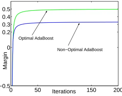
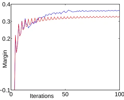
In Figure 8, we illustrate the evolution of margins in the optimal and non-optimal cases for matrix M of Theorem 6. Here, optimal AdaBoost converges to a margin of 1/2 via convergence to a 4-cycle, and non-optimal AdaBoost converges to a margin of 1/3 via convergence to a 3-cycle.

9. Optimal AdaBoost Does Not Necessarily Converge to a Maximum Margin Solution

0 50 150 200 −0.5

0 0.2 0.3 0.4 0.5

Iterations

Margin

Optimal AdaBoost

Non−Optimal AdaBoost

Figure 8: AdaBoost in the optimal case (higher curve) and in the non-optimal case (lower curve). Optimal AdaBoost converges to a margin of 1/2 via convergence to a 4-cycle, and non-optimal AdaBoost converges to a margin of 1/3 via convergence to a 3-cycle. In both cases we start withλ1=0.

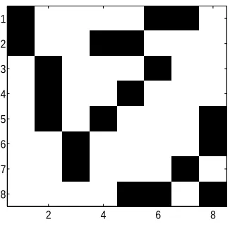
Theorem 7 Consider the following matrix whose image appears in Figure 9 (one can see the

nat-ural symmetry more easily in the imaged version):

M=

           

−1 1 1 1 1 ₋1 ₋1 1

−1 1 1 ₋1 ₋1 1 1 1

1 ₋1 1 1 1 ₋1 1 1 1 −1 1 1 −1 1 1 1 1 ₋1 1 ₋1 1 1 1 ₋1 1 1 ₋1 1 1 1 1 ₋1 1 1 −1 1 1 1 −1 1 1 1 1 1 ₋1 ₋1 1 ₋1

           

. (6)

For this matrix, it is possible for AdaBoost to fail to converge to a maximum margin solution.

Proof The dynamical system corresponding to this matrix contains a manifold of strongly attracting

3-cycles. The cycles we will analyze alternate between weak classifiers 3, 2, and 1. If we consider only weak classifiers 1, 2, and 3, we find that training examples i=1 and 2 are identically classified, i.e., rows 1 and 2 of matrix M are the same (only considering columns 1, 2, and 3). Similarly, examples 3, 4 and 5 are identically classified, and additionally, examples 6 and 7. Training example 8 is correctly classified by each of these weak classifiers. Because we have constructed M to have such a strong attraction to a 3-cycle, there are many initial conditions (initial values ofλ) for which AdaBoost will converge to one of these cycles, including the vectorλ=0. For the first iteration,

2 4 6 8 1 2 3 4 5 6 7 8

Figure 9: The image of the matrix M in (6). White indicates +1, black indicates -1. This matrix has natural symmetry.

a cycle in which a maximum margin solution is produced, although finding such a cycle requires some work.)

To show that a manifold of 3-cycles exists, we present a vector d1such that d4=d1, namely:

d1=

3₋√5 8 ,

3₋√5 8 , 1 6, 1 6, 1 6, √

5₋1 8 ,

√

5₋1 8 ,0

!T

. (7)

To see this, we iterate the iterated map 4 times.

dT₁M =

√

5₋1 2 ,0,

3₋√5 2 ,

3√5₋1 12 ,

3√5₋1 12 ,

3√5₋1 12 ,

1 2,

11₋3√5 12

!

,

and here j1=1,

d2 = 1 4,

1 4,

√

5₋1 12 ,

√

5₋1 12 ,

√

5₋1 12 ,

3₋√5 8 ,

3₋√5 8 ,0

!T

dT₂M = 0,3−

√

5 2 ,

√

5₋1 2 ,

4₋√5 6 ,

4₋√5 6 ,

4₋√5 6 ,

√

5₋1 4 ,

5+√5 12

!

,

and here j2=3,

d3 =

√

5₋1 8 ,

√

5₋1 8 ,

3₋√5 12 ,

3₋√5 12 ,

3₋√5 12 ,

1 4,

1 4,0

!T

dT₃M = 3−

√

5 2 ,

√

5₋1 2 ,0,

3 4− √ 5 12, 3 4− √ 5 12, 3 4− √ 5 12,

3₋√5 4 , √ 5 6 ! ,