In memory of Alexey Chervonenkis
Learning Using Privileged Information:
Similarity Control and Knowledge Transfer
Vladimir Vapnik [email protected]
Columbia University New York, NY 10027, USA Facebook AI Research New York, NY 10017, USA
Rauf Izmailov [email protected]
Applied Communication Sciences Basking Ridge, NJ 07920-2021, USA
Editor:Alex Gammerman and Vladimir Vovk
Abstract
This paper describes a new paradigm of machine learning, in which Intelligent Teacher is involved. During training stage, Intelligent Teacher provides Student with information that contains, along with classification of each example, additional privileged information (for example, explanation) of this example. The paper describes two mechanisms that can be used for significantly accelerating the speed of Student’s learning using privileged information: (1) correction of Student’s concepts of similarity between examples, and (2) direct Teacher-Student knowledge transfer.
Keywords: intelligent teacher, privileged information, similarity control, knowledge transfer, knowledge representation, frames, support vector machines, SVM+, classification, learning theory, kernel functions, similarity functions, regression
1. Introduction
During the last fifty years, a strong machine learning theory has been developed. This theory (see Vapnik and Chervonenkis, 1974, Vapnik, 1995, Vapnik, 1998, Chervonenkis, 2013) includes:
• The necessary and sufficient conditions for consistency of learning processes.
• The bounds on the rate of convergence, which, in general, cannot be improved.
• The new inductive principle called Structural Risk Minimization (SRM), which always converges to the best possible approximation in the given set of functions1.
• The effective algorithms, such as Support Vector Machines (SVM), that realize the consistency property of SRM principle2.
The general learning theory appeared to be completed: it addressed almost all standard questions of the statistical theory of inference. However, as always, the devil is in the detail: it is a common belief that human students require far fewer training examples than any learning machine. Why?
We are trying to answer this question by noting that a human Student has an Intelligent Teacher3 and that Teacher-Student interactions are based not only on brute force methods of function estimation. In this paper, we show that Teacher-Student interactions can include special learning mechanisms that can significantly accelerate the learning process. In order for a learning machine to use fewer observations, it can use these mechanisms as well.
This paper considers a model of learning with the so-called Intelligent Teacher, who supplies Student with intelligent (privileged) information during training session. This is in contrast to the classical model, where Teacher supplies Student only with outcome yfor eventx.
Privileged information exists for almost any learning problem and this information can significantly accelerate the learning process.
2. Learning with Intelligent Teacher: Privileged Information
The existing machine learning paradigm considers a simple scheme: given a set of training examples, find, in a given set of functions, the one that approximates the unknown decision rule in the best possible way. In such a paradigm, Teacher does not play an important role. In human learning, however, the role of Teacher is important: along with examples, Teacher provides students with explanations, comments, comparisons, metaphors, and so on. In the paper, we include elements of human learning into classical machine learning paradigm. We consider a learning paradigm called Learning Using Privileged Information (LUPI), where, at the training stage, Teacher provides additional information x∗ about training example x.
The crucial point in this paradigm is that the privileged information is available only at the training stage (when Teacher interacts with Student) and is not available at the test stage (when Student operates without supervision of Teacher).
In this paper, we consider two mechanisms of Teacher–Student interactions in the frame-work of the LUPI paradigm:
1. The mechanism to control Student’s concept of similarity between training exam-ples.
strongly uniformly converges to the function f(x, α0) that minimizes the error rate on the closure of
∪∞k=1Sk(Vapnik and Chervonenkis, 1974), (Vapnik, 1982), (Devroye et al., 1996), (Vapnik, 1998). 2. Solutions of SVM belong to Reproducing Kernel Hilbert Space (RKHS). Any subset of functions in
RKHS with bounded norm has a finite VC dimension. Therefore, SRM with respect to the value of norm of functions satisfies the general SRM model of strong uniform convergence. In SVM, the element of SRM structure is defined by parameterC of SVM algorithm.
2. The mechanism to transfer knowledge from the space of privileged information (space of Teacher’s explanations) to the space where decision rule is constructed.
The first mechanism (Vapnik, 2006) was introduced in 2006 using SVM+ method. Here we reinforce SVM+ by constructing a parametric family of methods SVM∆+; for ∆ =
∞, the method SVM∆+ is equivalent to SVM+. The first experiments with privileged information using SVM+ method were described in Vapnik and Vashist (2009); later, the method was applied to a number of other examples (Sharmanska et al., 2013; Ribeiro et al., 2012; Liang and Cherkassky, 2008).
The second mechanism was introduced recently (Vapnik and Izmailov, 2015b).
2.1 Classical Model of Learning
Formally, the classical paradigm of machine learning is described as follows: given a set of iid pairs (training data)
(x1, y1), ...,(x`, y`), xi∈X, yi ∈ {−1,+1}, (1)
generated according to a fixed but unknown probability measure P(x, y), find, in a given set of indicator functions f(x, α), α ∈ Λ, the function y = f(x, α∗) that minimizes the probability of incorrect classifications (incorrect values of y ∈ {−1,+1}). In this model, each vector xi ∈ X is a description of an example generated by Nature according to an
unknown generatorP(x) of random vectorsxi, andyi ∈ {−1,+1}is its classification defined
according to a conditional probability P(y|x). The goal of Learning Machine is to find the function y = f(x, α∗) that guarantees the smallest probability of incorrect classifications. That is, the goal is to find the function which minimizes the risk functional
R(α) = 1 2
Z
|y−f(x, α)|dP(x, y) (2)
in the given set of indicator functionsf(x, α), α∈Λ when the probability measureP(x, y) =
P(y|x)P(x) is unknown but training data (1) are given.
2.2 LUPI Paradigm of Learning
The LUPI paradigm describes a more complex model: given a set of iid triplets
(x1, x∗1, y1), ...,(x`, x∗`, y`), xi ∈X, x∗i ∈X
∗
, yi ∈ {−1,+1}, (3)
generated according to a fixed but unknown probability measure P(x, x∗, y), find, in a given set of indicator functions f(x, α), α ∈ Λ, the function y =f(x, α∗) that guarantees the smallest probability of incorrect classifications (2).
In the LUPI paradigm, we have exactly the same goal of minimizing (2) as in the classical paradigm, i.e., to find the best classification function in the admissible set. However, during the training stage, we have more information, i.e., we have triplets (x, x∗, y) instead of pairs (x, y) as in the classical paradigm. The additional information x∗ ∈ X∗ belongs to space
X∗, which is, generally speaking, different from X. For any element (xi, yi) of training
example generated by Nature, Intelligent Teacher generates the privileged information x∗i
In this paper, we first illustrate the work of these mechanisms on SVM algorithms; after that, we describe their general nature.
Since the additional information is available only for the training set andis notavailable for the test set, it is calledprivileged information and the new machine learning paradigm is called Learning Using Privileged Information.
Next, we consider three examples of privileged information that could be generated by Intelligent Teacher.
Example 1. Suppose that our goal is to find a rule that predicts the outcome y of a surgery in three weeks after it, based on information x available before the surgery. In order to find the rule in the classical paradigm, we use pairs (xi, yi) from previous patients.
However, for previous patients, there is also additional informationx∗ about procedures and complications during surgery, development of symptoms in one or two weeks after surgery, and so on. Although this information is not available before surgery, it does exist in historical data and thus can be used as privileged information in order to construct a rule that is better than the one obtained without using that information. The issue is how large an improvement can be achieved.
Example 2. Let our goal be to find a ruley=f(x) to classify biopsy imagesxinto two categories y: cancer (y = +1) and non-cancer (y =−1). Here images are in a pixel space
X, and the classification rule has to be in the same space. However, the standard diagnostic procedure also includes a pathologist’s report x∗ that describes his/her impression about the image in a high-level holistic languageX∗ (for example, “aggressive proliferation of cells of typeA among cells of type B” etc.).
The problem is to use the pathologist’s reportsx∗ as privileged information (along with images x) in order to make a better classification rule for images x just in pixel space
X. (Classification by a pathologist is a time-consuming procedure, so fast decisions during surgery should be made without consulting him or her).
Example 3. Let our goal be to predict the direction of the exchange rate of a currency at the momentt. In this problem, we have observations about the exchange rates before t, and we would like to predict if the rate will go up or down at the moment t+ ∆. However, in the historical market data we also have observations about exchange ratesaftermoment
t. Can this future-in-the-past privileged information be used for construction of a better prediction rule?
To summarize, privileged information is ubiquitous: it usually exists for almost any machine learning problem.
Section 4 describes the first mechanism that allows one to take advantage of privileged information by controlling Student’s concepts of similarity between training examples. Sec-tion 5 describes examples where LUPI model uses similarity control mechanism. SecSec-tion 6 is devoted to mechanism of knowledge transfer from space of privileged information X∗
into decision space X.
3. Statistical Analysis of the Rate of Convergence
According to the bounds developed in the VC theory (Vapnik and Chervonenkis, 1974), (Vapnik, 1998), the rate of convergence depends on two factors: how well the classification rule separates the training data
(x1, y1), ...,(x`, y`), x∈Rn, y∈ {−1,+1}, (4)
and the VC dimension of the set of functions in which the rule is selected. The theory has two distinct cases:
1. Separable case: there exists a functionf(x, α`) in the set of functionsf(x, α), α∈Λ
with finite VC dimensionh that separates the training data (4) without errors:
yif(xi, α`)>0 ∀i= 1, ..., `.
In this case, for the functionf(x, α`) that minimizes (down to zero) the empirical risk
(on training set (4)), the bound
P(yf(x, α`)≤0)< O∗
h−lnη `
holds true with probability 1−η, where P(yf(x, α`) ≤0) is the probability of error
for the functionf(x, α`) andhis the VC dimension of the admissible set of functions.
Here O∗ denotes order of magnitude up to logarithmic factor.
2. Non-separable case: there is no function in f(x, α), α∈Λ finite VC dimension h
that can separate data (4) without errors. Let f(x, α`) be a function that minimizes
the number of errors on (4). Let ν(α`) be its error rate on training data (4). Then,
according to the VC theory, the following bound holds true with probability 1−η:
P(yf(x, α`)≤0)< ν(α`) +O∗
r
h−lnη `
!
.
In other words, in the separable case, the rate of convergence has the order of magnitude 1/`; in the non-separable case, the order of magnitude is 1/√`. The difference between these rates4 is huge: the same order of bounds requires 320 training examples versus 100,000 examples. Why do we have such a large gap?
3.1 Key Observation: SVM with Oracle Teacher
Let us try to understand why convergence rates for SVMs differ so much for separable and non-separable cases. Consider two versions of the SVM method for these cases.
SVM method first maps vectors x of space X into vectors z of space Z and then con-structs a separating hyperplane in space Z. If training data can be separated with no error (the so-called separable case), SVM constructs (in space Z that we, for simplicity,
consider as anN-dimensional vector spaceRN) a maximum margin separating hyperplane. Specifically, in the separable case, SVM minimizes the functional
T(w) = (w, w)
subject to the constraints
(yi(w, zi) +b)≥1, ∀i= 1, ..., `;
whereas in the non-separable case, SVM minimizes the functional
T(w) = (w, w) +C
`
X
i=1
ξi
subject to the constraints
(yi(w, zi) +b)≥1−ξi, ∀i= 1, ..., `,
where ξi ≥0 are slack variables. That is, in the separable case, SVM uses ` observations
for estimation ofN coordinates of vectorw, whereas in the nonseparable case, SVM uses`
observations for estimation ofN+`parameters: N coordinates of vectorwand `values of slacksξi. Thus, in the non-separable case, the number N+`of parameters to be estimated
is always larger than the number ` of observations; it does not matter here that most of slacks will be equal to zero: SVM still has to estimate all `of them. Our guess is that the difference between the corresponding convergence rates is due to the number of parameters SVM has to estimate.
To confirm this guess, consider the SVM with Oracle Teacher (Oracle SVM). Suppose that Teacher can supply Student with the values of slacks as privileged information: during training session, Student is supplied with triplets
(x1, ξ10, y1), ...,(x`, ξ`0, y`),
where ξi0, i = 1, ..., ` are the slacks for the Bayesian decision rule. Therefore, in order to construct the desired rule using these triplets, the SVM has to minimize the functional
T(w) = (w, w)
subject to the constraints
(yi(w, zi) +b)≥ri, ∀i= 1, ..., `,
where we have denoted
ri= 1−ξi0, ∀i= 1, ..., `.
Proposition 1. Letf(x, α0)be a function from the set of indicator functionsf(x, α),
withα∈Λ with VC dimension h that minimizes the frequency of errors (on this set) and let
ξi0 = max{0,(1−f(xi, α0))}, ∀i= 1, ..., `.
Then the error probability p(α`)for the function f(x, α`) that satisfies the constraints
yif(x, α)≥1−ξi0, ∀i= 1, ..., `
is bounded, with probability 1−η, as follows:
p(α`)≤P(1−ξ0 <0) +O∗
h−lnη `
.
3.2 From Ideal Oracle to Real Intelligent Teacher
Of course, real Intelligent Teacher cannot supply slacks: Teacher does not know them. Instead, Intelligent Teacher can do something else, namely:
1. define a spaceX∗ of (correcting) slack functions (it can be different from the space
X of decision functions);
2. define a set of real-valued slack functions f∗(x∗, α∗), x∗ ∈ X∗, α∗ ∈Λ∗ with VC dimensionh∗, where approximations
ξi=f∗(x, α∗)
of the slack functions5 are selected;
3. generate privileged information for training examples supplying Student, instead of pairs (4), with triplets
(x1, x∗1, y1), ...,(x`, x∗`, y`). (5)
During training session, the algorithm has to simultaneously estimate two functions using triplets (5): the decision functionf(x, α`) and the slack functionf∗(x∗, α∗`). In other words,
the method minimizes the functional
T(α∗) =
`
X
i=1
max{0, f∗(x∗i, α∗)} (6)
subject to the constraints
yif(xi, α)>−f∗(x∗i, α
∗
), i= 1, ..., `. (7)
Letf(x, α`) andf∗(x∗, α∗`) be functions that solve this optimization problem. For these
functions, the following proposition holds true (Vapnik and Vashist, 2009).
Proposition 2. The solution f(x, α`) of optimization problem (6), (7) satisfies the
bounds
P(yf(x, α`)<0)≤P(f∗(x∗, α∗`)≥0) +O
∗
h+h∗−lnη `
with probability 1−η, where h and h∗ are the VC dimensions of the set of decision functions f(x, α), α ∈ Λ, and the set of correcting functions f∗(x∗, α∗), α∗ ∈ Λ∗, respectively.
According to Proposition 2, in order to estimate the rate of convergence to the best possi-ble decision rule (in spaceX) one needs to estimate the rate of convergence ofP{f∗(x∗, α∗`)≥ 0} toP{f∗(x∗, α∗0)≥0} for the best rulef∗(x∗, α∗0) in spaceX∗. Note that both the space
X∗ and the set of functions f∗(x∗, α∗`), α∗ ∈ Λ∗ are suggested by Intelligent Teacher that tries to choose them in a way that facilitates a fast rate of convergence. The guess is that a really Intelligent Teacher can indeed do that.
As shown in the VC theory, in standard situations, the uniform convergence has the orderO∗(ph∗/`), whereh∗is the VC dimension of the admissible set of correcting functions
f∗(x∗, α∗),α∗ ∈Λ∗. However, for special privileged space X∗ and corresponding functions
f∗(x∗, α∗), α∗∈Λ∗, the convergence can be faster (as O∗([1/`]δ), δ >1/2).
A well-selected privileged information spaceX∗and Teacher’s explanationP(x∗|x) along with sets {f(x, α`), α ∈ Λ} and {f∗(x∗, α∗), α∗ ∈ Λ∗} engender a convergence that is
faster than the standard one. The skill of Intelligent Teacher is being able to select of the proper space X∗, generator P(x∗|x), set of functions f(x, α`), α∈ Λ, and set of
func-tionsf∗(x∗, α∗), α∗∈Λ∗: that is what differentiates good teachers from poor ones.
4. Similarity Control in LUPI Paradigm
4.1 SVM∆+ for Similarity Control in LUPI Paradigm
In this section, we extend SVM method of function estimation to the method called SVM+, which allows one to solve machine learning problems in the LUPI paradigm (Vapnik, 2006). The SVMε+ method presented below is a reinforced version of the one described in Vapnik
(2006) and used in Vapnik and Vashist (2009).
Consider the model of learning with Intelligent Teacher: given triplets
(x1, x∗1, y1), ...,(x`, x∗`, y`),
find in the given set of functions the one that minimizes the probability of incorrect classi-fications in spaceX.
As in standard SVM, we map vectors xi∈X onto the elementszi of the Hilbert space
Z, and map vectors x∗i onto elements zi∗ of another Hilbert spaceZ∗ obtaining triples
(z1, z1∗, y1), ...,(z`, z∗`, y`).
Let the inner product in spaceZ be (zi, zj), and the inner product in spaceZ∗ be (z∗i, zj∗).
Consider the set of decision functions in the form
wherew is an element in Z, and consider the set of correcting functions in the form
ξ∗(x∗, y) = [y((w∗, z∗) +b∗)]+,
wherew∗ is an element in Z∗ and [u]+= max{0, u}.
Our goal is to we minimize the functional
T(w, w∗, b, b∗) = 1
2[(w, w) +γ(w ∗
, w∗)] +C
`
X
i=1
[yi((w∗, zi∗) +b
∗ )]+
subject to the constraints
yi[(w, zi) +b]≥1−[yi((w∗, zi∗)−b
∗ )]+.
The structure of this problem mirrors the structure of the primal problem for standard SVM. However, due to the elements [ui]+ = max{0, ui} that define both the objective
function and the constraints here we faced non-linear optimization problem.
To find the solution of this optimization problem, we approximate this non-linear opti-mization problem with the following quadratic optiopti-mization problem: minimize the func-tional
T(w, w∗, b, b∗) = 1
2[(w, w) +γ(w ∗
, w∗)] +C
`
X
i=1
[yi((w∗, zi∗) +b
∗
) +ζi] + ∆C `
X
i=1
ζi (8)
(here ∆>0 is the parameter of approximation6) subject to the constraints
yi((w, zi) +b)≥1−yi((w∗, z∗) +b∗)−ζi, i= 1, ..., `, (9)
the constraints
yi((w∗, zi∗) +b
∗) +ζ
i ≥0, ∀i= 1, ..., `, (10)
and the constraints
ζi ≥0, ∀i= 1, ..., `. (11)
To minimize the functional (8) subject to the constraints (10), (11), we construct the La-grangian
L(w, b, w∗, b∗, α, β) = (12)
1
2[(w, w) +γ(w ∗
, w∗)] +C
`
X
i=1
[yi((w∗, zi∗) +b
∗
) + (1 + ∆)ζi]− `
X
i=1
νiζi −
`
X
i=1
αi[yi[(w, zi) +b]−1 + [yi((w∗, zi∗) +b
∗) +ζ
i]]− `
X
i=1
βi[yi((w∗, z∗i) +b
∗) +ζ
i],
whereαi≥0, βi≥0, νi≥0, i= 1, ..., ` are Lagrange multipliers.
To find the solution of our quadratic optimization problem, we have to find the saddle point of the Lagrangian (the minimum with respect to w, w∗, b, b∗ and the maximum with respect toαi, βi, νi, i= 1, ..., `).
The necessary conditions for minimum of (12) are
∂L(w, b, w∗, b∗, α, β)
∂w = 0 =⇒ w=
`
X
i=1
αiyizi (13)
∂L(w, b, w∗, b∗, α, β)
∂w∗ = 0 =⇒ w
∗ = 1
γ
`
X
i=1
yi(αi+βi−C)zi∗ (14)
∂L(w, b, w∗, b∗, α, β)
∂b = 0 =⇒
`
X
i=1
αiyi = 0 (15)
∂L(w, b, w∗, b∗, α, β)
∂b∗ = 0 =⇒
`
X
i=1
yi(C−αi−βi) = 0 (16)
∂L(w, b, w∗, b∗, α, β)
∂ζi
= 0 =⇒ αi+βi+νi= (C+ ∆C) (17)
Substituting the expressions (13) in (12) and, taking into account (14), (15), (16), and denotingδi=C−βi, we obtain the functional
L(α, δ) =
`
X
i=1
αi−
1 2
`
X
i,j=1
(zi, zj)yiyjαiαj −
1 2γ
`
X
i,j=1
(δi−αi)(δj−αj)(zi∗, z∗j)yiyj.
To find its saddle point, we have to maximize it subject to the constraints7
`
X
i=1
yiαi = 0 (18)
`
X
i=1
yiδi= 0 (19)
0≤δi ≤C, i= 1, ..., ` (20)
0≤αi≤δi+ ∆C, i= 1, ..., ` (21)
Let vectorsα0, δ0 be a solution of this optimization problem. Then, according to (13) and (14), one can find the approximations to the desired decision function
f(x) = (w0, zi) +b= `
X
i=1
α∗iyi(zi, z) +b
and to the slack function
ξ∗(x∗, y) =yi((w∗0, z
∗
i) +b
∗
) +ζ =
`
X
i=1
yi(α0i −δ0i)(z
∗
i, z
∗
) +b∗+ζ.
The Karush-Kuhn-Tacker conditions for this problem are α0
i[yi[(w0, zi) +b+ (w0∗, zi∗) +b∗] +ζi−1] = 0
(C−δ0i)[(w0∗, z∗i) +b∗+ζi] = 0
νi0ζi = 0
Using these conditions, one obtains the value of constantb as
b= 1−yk(w0, zk) = 1−yk
" ` X
i=1
α0i(zi, zk)
#
,
where (zk, zk∗, yk) is a triplet for whichαk0 6= 0, δk06=C,zi 6= 0.
As in standard SVM, we use the inner product (zi, zj) in space Z in the form of
Mer-cer kernel K(xi, xj) and inner product (zi∗, z∗j) in space Z∗ in the form of Mercer kernel
K∗(x∗i, x∗j). Using these notations, we can rewrite the SVM∆+ method as follows: the
decision rule in X space has the form
f(x) =
`
X
i=1
yiα0iK(xi, x) +b,
where K(·,·) is the Mercer kernel that defines the inner product for the image space Z of space X (kernel K∗(·,·) for the image space Z∗ of space X∗) and α0 is a solution of the following dual space quadratic optimization problem: maximize the functional
L(α, δ) =
`
X
i=1
αi−
1 2
`
X
i,j=1
yiyjαiαjK(xi, xj)−
1 2γ
`
X
i,j=1
yiyj(αi−δi)(αj−δj)K∗(x∗i, x∗j)
subject to constraints (18) – (21).
Remark. Note that if δi = αi or ∆ = 0, the solution of our optimization problem
becomes equivalent to the solution of the standard SVM optimization problem, which max-imizes the functional
L(α, δ) =
`
X
i=1
αi−
1 2
`
X
i,j=1
yiyjαiαjK(xi, xj)
subject to constraints (18) – (21) whereδi=αi.
Therefore, the difference between SVM∆+ and SVM solutions is defined by the last
term in objective function (8). In SVM method, the solution depends only on the values of pairwise similarities between training vectors defined by the Gram matrixK of elements
K(xi, xj) (which defines similarity between vectors xi and xj). The SVM∆+ solution is
defined by objective function (8) that uses two expressions of similarities between observa-tions: one (K(xi, xj) for xi andxj) that comes from spaceX and another one (K∗(x∗i, x∗j)
The last term in equation (8) defines the instrument for Intelligent Teacher to control the concept of similarity of Student.
Efficient computational implementation of this SVM+ algorithm for classification and its extension for regression can be found in Pechyony et al. (2010) and Vapnik and Vashist (2009), respectively.
4.1.1 Simplified Approach
The described methodSV M∆+ requires to minimize the quadratic formL(α, δ) subject to
constraints (18) – (21). For large`it can be a challenging computational problem. Consider the following approximation. Let
f∗(x∗, α∗`) =
`
X
i=1
α∗iK∗(x∗i, x) +b∗
be be an SVM solution in space X∗ and let
ξi∗ = [1−f∗(x∗, α∗`)−b∗]+
be the corresponding slacks. Let us use the linear function
ξi=tξ∗i +ζi, ζi ≥0
as an approximation of slack function in space X. Now we minimize the functional
(w, w) +C
`
X
i=1
(tξi∗+ (1 + ∆)ζi), ∆≥0
subject to the constraints
yi((w, zi) +b)>1−tξi∗+ζi,
t >0, ζi ≥0, i= 1, ..., `
(here zi is Mercer mapping of vectorsxi in RKHS).
The solution of this quadratic optimization problem defines the function
f(x, α`) = `
X
i=1
αiK(xi, x) +b,
whereα is solution of the following dual problem: maximize the functional
R(α) =
`
X
i=1
αi−
1 2
`
X
i,j=1
αiαjyiyjK(xi, xj)
subject to the constraints
`
X
i=1
yiαi = 0
`
X
i=1
αiξi∗ ≤C `
X
i=1
ξi∗
4.2 General Form of Similarity Control in LUPI Paradigm
Consider the following two sets of functions: the set f(x, α), α ∈ Λ defined in space X
and the set f∗(x∗, α∗), α∗ ∈Λ∗, defined in space X∗. Let a non-negative convex functional Ω(f) ≥ 0 be defined on the set of functions f(x, α), α ∈ Λ, while a non-negative convex functional Ω∗(f∗) ≥ 0 be defined on the set of functions f(x∗, α∗), α∗ ∈ Λ∗. Let the sets of functions θ(f(x, α)), α ∈ Λ, and θ(f(x∗, α∗)), α∗ ∈ Λ∗, which satisfy the corresponding bounded functionals
Ω(f)≤Ck
Ω∗(f∗)≤Ck,
have finite VC dimensionshk and hk, respectively. Consider the structures
S1⊂...⊂Sm....
S∗1 ⊂...⊂Sm∗...
defined on corresponding sets of functions. Let iid observations of triplets
(x1, x∗1, y1), ...,(x`, x∗`, y`)
be given. Our goal is to find the functionf(x, α`) that minimizes the probability of the test
error.
To solve this problem, we minimize the functional
`
X
i=1
f∗(x∗i, α)
subject to constraints
yi[f(x, α) +f(x∗, α∗)]>1
and the constraint
Ω(f) +γΩ(f∗)≤Cm
(we assume that our sets of functions are such that solutions exist).
Then, for any fixed setsSkandSk∗, the VC bounds hold true, and minimization of these
bounds with respect to both sets Sk and Sk∗ of functions and the functions f(x, α`) and
f∗(x(, α∗
`) in these sets is a realization of universally consistent SRM principle.
The sets of functions defined in previous section by the Reproducing Kernel Hilbert Space satisfy this model since any subset of functions from RKHS with bounded norm has finite VC dimension according to the theorem about VC dimension of linear bounded functions in Hilbert space8.
5. Transfer of Knowledge Obtained in Privileged Information Space to Decision Space
In this section, we consider the second important mechanism of Teacher-Student interaction: using privileged information for knowledge transfer from Teacher to Student9.
Suppose that Intelligent Teacher has some knowledge about the solution of a specific pattern recognition problem and would like to transfer this knowledge to Student. For example, Teacher can reliably recognize cancer in biopsy images (in a pixel space X) and would like to transfer this skill to Student.
Formally, this means that Teacher has some functiony=f0(x) that distinguishes cancer
(f0(x) = +1 for cancer andf0(x) =−1 for non-cancer) in the pixel spaceX. Unfortunately,
Teacher does not know this function explicitly (it only exists as a neural net in Teacher’s brain), so how can Teacher transfer this construction to Student? Below, we describe a possible mechanism for solving this problem; we call this mechanismknowledge transfer.
Suppose that Teacher believes in some theoretical model on which the knowledge of Teacher is based. For cancer model, he or she believes that it is a result of uncontrolled multiplication of the cancer cells (cells of type B) that replace normal cells (cells of type A). Looking at a biopsy image, Teacher tries to generate privileged information that reflects his or her belief in development of such process; Teacher may describe the image as:
Aggressive proliferation of cells of type B into cells of type A.
If there are no signs of cancer activity, Teacher may use the description
Absence of any dynamics in the of standard picture.
In uncertain cases, Teacher may write
There exist small clusters of abnormal cells of unclear origin.
In other words, Teacher has developed a special language that is appropriate for de-scription x∗i of cancer development based on the model he or she believes in. Using this language, Teacher supplies Student with privileged information x∗i for the image xi by
generating training triplets
(x1, x∗1, y1), ...,(x`, x∗`, y`). (22)
The first two elements of these triplets are descriptions of an image in two languages: in language X (vectors xi in pixel space), and in language X∗ (vectors x∗i in the space of
privileged information), developed for Teacher’s understanding of cancer model.
Note that the language of pixel space is universal (it can be used for description of many different visual objects; for example, in the pixel space, one can distinguish between male and female faces), while the language used for describing privileged information is very specific: it reflects just a model of cancer development. This has an important consequence:
the set of admissible functions in spaceX has to be rich (has a large VC dimension), while the set of admissible functions in spaceX∗ may be not rich (has a small VC dimension).
One can consider two related pattern recognition problems using triplets (22):
1. The problem of constructing a rule y = f(x) for classification of biopsy in the pixel space X using data
(x1, y1), ...,(x`, y`). (23)
2. The problem of constructing a ruley=f∗(x∗) for classification of biopsy in the space
X∗ using data
(x∗1, y1), ...,(x∗`, y`). (24)
Suppose that language X∗ is so good that it allows to create a rule y = f`∗(x∗) that classifies vectorsx∗ corresponding to vectors x with the same level of accuracy as the best rule y=f`(x) for classifying data in the pixel space10.
In the considered example, the VC dimension of the admissible rules in a special space
X∗ is much smaller than the VC dimension of the admissible rules in the universal space
X and, since the number of examples `is the same in both cases, the bounds on the error rate for the rule y = f`∗(x∗) in X∗ will be better11 than those for the rule y = f`(x) in
X. Generally speaking, the knowledge transfer approach can be applied if the classification rule y=f`∗(x∗) is more accurate than the classification rule y=f`(x) (the empirical error
in privileged space is smaller than the empirical error in the decision space). The following problem arises: how one can use the knowledge of the rule
y=f`∗(x∗) in space X∗ to improve the accuracy of the desired rule y=f`(x) in spaceX?
5.1 Knowledge Representation for SVMs
To answer this question, we formalize the concept of representation of the knowledge about the rule y=f`∗(x∗).
Suppose that we are looking for our rule in Reproducing Kernel Hilbert Space (RKHS) associated with kernel K∗(x∗i, x∗). According to Representer Theorem (Kimeldorf and Wahba, 1971; Sch¨olkopf et al., 2001), such rule has the form
f`∗(x∗) =
`
X
i=1
γiK∗(x∗i, x∗) +b, (25)
whereγi, i= 1, ..., ` andb are parameters.
Suppose that, using data (24), we found a good rule (25) with coefficients γi=γi∗, i=
1, ..., ` and b = b∗. This is now the knowledge about our classification problem. Let us formalize the description of this knowledge.
Consider three elements of knowledge representation used in Artificial Intelligence (Brach-man and Levesque, 2004):
10. The rule constructed in space X∗ cannot be better than the best possible rule in space X, since all information originates in spaceX.
1. Fundamental elements of knowledge.
2. Frames (fragments) of the knowledge.
3. Structural connections of the frames (fragments) in the knowledge.
We call thefundamental elements of the knowledgea limited number of vectorsu∗1...., u∗m
from spaceX∗that can approximate well the main part of rule (25). It could be the support vectors or the smallest number of vectors12 u
i ∈X∗:
f`∗(x∗)−b=
`
X
i=1
γ∗iK∗(x∗i, x∗)≈
m
X
k=1
βk∗K∗(u∗k, x∗). (26)
Let us call the functionsK∗(u∗k, x∗), k= 1, ..., mtheframes(fragments) of knowledge. Our knowledge
f`∗(x∗) =
m
X
k=1
βk∗K∗(u∗k, x∗) +b
is defined as a linear combination of the frames.
5.1.1 Scheme of Knowledge Transfer Between Spaces
In the described terms, knowledge transfer from X∗ intoX requires the following:
1. To find the fundamental elements of knowledgeu∗1, ..., u∗m in spaceX∗. 2. To find frames (m functions) K∗(u∗1, x∗), ..., K∗(u∗m, x∗) in space X∗. 3. To find the functionsφ1(x), ..., φm(x) in space X such that
φk(xi)≈K∗(u∗k, x
∗
i) (27)
holds true for almost all pairs (xi, x∗i) generated by Intelligent Teacher that uses some
(unknown) generatorP(x∗, x) =P(x∗|x)P(x).
Note that the capacity of the set of functions from which φk(x) are to be chosen can be
smaller than that of the capacity of the set of functions from which the classification function
y =f`(x) is chosen (function φk(x) approximates just one fragment of knowledge, not the
entire knowledge, as function y = f`∗(x∗), which is a linear combination (26) of frames). Also, as we will see in the next section, estimates of all the functions φ1(x), ..., φm(x) are
done using different pairs as training sets of the same size`. That is, we hope that transfer ofmfragments of knowledge from spaceX∗ into spaceX can be done with higher accuracy than estimating the function y=f`(x) from data (23).
After finding images of frames in space X, the knowledge about the rule obtained in space X∗ can be approximated in space X as
f`(x)≈ m
X
k=1
δkφk(x) +b∗,
where coefficientsδk=γk(taken from (25)) if approximations (27) are accurate. Otherwise,
coefficients δk can be estimated from the training data, as shown in Section 6.3.
5.1.2 Finding the Smallest Number of Fundamental Elements of Knowledge
Let our functions φ belong to RKHS associated with the kernel K∗(x∗i, x∗), and let our knowledge be defined by an SVM method in space X∗ with support vector coefficients αi.
In order to find the smallest number of fundamental elements of knowledge, we have to minimize (over vectorsu∗1, ..., u∗m and values β1, ..., βm) the functional
R(u∗1, ..., u∗m;β1, ..., βm) = (28)
` X i=1
yiαiK∗(x∗i, x
∗)−
m
X
s=1
βsK∗(u∗s, x
∗) 2 RKHS = ` X i,j=1
yiyjαiαjK∗(x∗i, x
∗
j)−2 ` X i=1 m X s=1
yiαiβsK∗(x∗i, u
∗
s) + m
X
s,t=1
βsβtK∗(u∗s, u
∗
t).
The last equality was derived from the following property of the inner product for functions in RKHS (Kimeldorf and Wahba, 1971; Sch¨olkopf et al., 2001):
K∗(x∗i, x∗), K(x∗j, x∗)
RKHS =K
∗(x∗
i, x∗j).
5.1.3 Smallest Number of Fundamental Elements of Knowledge for Homogeneous Quadratic Kernel
For general kernel functionsK∗(·,·), minimization of (28) is a difficult computational prob-lem. However, for the special homogeneous quadratic kernel
K∗(x∗i, x∗j) = (x∗i, x∗j)2,
this problem has a simple exact solution (Burges, 1996). For this kernel, we have
R=
`
X
i,j=1
yiyjαiαj(x∗i, x
∗
j)2−2 ` X i=1 m X s=1
yiαiβs(x∗i, u
∗
s)2+ m
X
s,t=1
βsβt(u∗s, u
∗
t)2. (29)
Let us look for solution in set of orthonormal vectors u∗i, ..., u∗m for which we can rewrite (29) as follows
ˆ
R=
`
X
i,j=1
yiyjαiαj(x∗i, x
∗
j)2−2 ` X i=1 m X s=1
yiαiβs(x∗i, u
∗
s)2+ m
X
s=1
βs2(u∗s, u∗s)2. (30)
Taking derivative of ˆR with respect to u∗k, we obtain that the solutions u∗k, k = 1, ..., m
have to satisfy the equations
dRˆ duk
=−2βk `
X
i=1
yiαix∗ix∗iTu∗k+ 2βk2u∗k= 0.
Introducing notation
S =
`
X
i=1
we conclude that the solutions satisfy the equation
Su∗k =βku∗k, k= 1, ..., m.
Let us chose from the setu∗1, ..., u∗mof eigenvectors of the matrixSthe vectors corresponding to the largest in absolute values eigenvaluesβ1, . . . , βm, which are coefficients of expansion
of the classification rule on the frames (uk, x∗)2, k= 1, . . . , m.
Using (31), one can rewrite the functional (30) in the form
ˆ
R=1TS21−
m
X
k=1
βk2, (32)
where we have denoted by S2 the matrix obtained from S with its elements si,j replaced
withs2i,j, and by 1 we have denoted the (`×1)-dimensional matrix of ones.
Therefore, in order to find the fundamental elements of knowledge, one has to solve the eigenvalue problem for (n×n)-dimensional matrixSand then select an appropriate number of eigenvectors corresponding to eigenvalues with largest absolute values. One chooses such
m eigenvectors for which functional (32) is small. The number m does not exceed n (the dimensionality of matrixS).
5.1.4 Finding Images of Frames in Space X
Let us call the conditional expectation function
φk(x) =
Z
K∗(u∗k, x∗)p(x∗|x)dx∗
the image of frame K∗(u∗k, x∗) in space X. To find m image functions φk(x) of the frames
K(u∗k, x∗), k= 1, ..., min spaceX, we solve the followingmregression estimation problems: find the regression function φk(x) in X,k= 1, . . . , m, using data
(x1, K∗(u∗k, x
∗
1)), ...,(x`, K∗(u∗k, x
∗
`)), k= 1, . . . , m, (33)
where pairs (xi, x∗i) belong to elements of training triplets (22).
Therefore, using fundamental elements of knowledge u∗1, ...u∗m in space X∗, the corre-sponding frames K∗(u∗1, x∗), ..., K∗(u∗m, x∗) in space X∗, and the training data (33), one constructs the transformation of the space X intom-dimensional feature space13
φ(x) = (φ1(x), ...φm(x)),
wherek-th coordinate of vector function φ(x) is defined asφk=φk(x).
5.1.5 Algorithms for Knowledge Transfer
1. Suppose that our regression functions can be estimated accurately: for a sufficiently small ε >0 the inequalities
|φk(xi)−K∗(u∗k, x
∗
i)|< ε, ∀k= 1, ..., m and ∀i= 1, ..., `
hold true for almost all pairs (xi, x∗i) generated according toP(x∗|y). Then the
approxima-tion of our knowledge in spaceX is
f(x) =
m
X
k=1
β∗kφk(x) +b∗,
whereβ∗k, k= 1, ..., mare eigenvalues corresponding to eigenvectors u∗1, ..., u∗m.
2. If, however, ε is not too small, one can use privileged information to employ both mechanisms of intelligent learning: controlling similarity between training examples and knowledge transfer.
In order to describe this method, we denote by vectorφi them-dimensional vector with
coordinates
φi = (φ1(xi), ..., φm(xi))T.
Consider the following problem of intelligent learning: given training triplets
(φ1, x∗1, y1), ...,(φ`, x∗`, y`),
find the decision rule
f(φ(x)) =
`
X
i=1
yiαˆiKˆ(φi, φ) +b. (34)
Using SVM∆+ algorithm described in Section 4, we can find the coefficients of expansion
ˆ
αi in (34). They are defined by the maximum (over ˆα andδ) of the functional
R( ˆα, δ) =
`
X
i=1
ˆ
αi−
1 2
`
X
i,j=1
yiyjαˆiαˆjKˆ(φi, φj)−
1 2γ
`
X
i,j=1
yiyj( ˆαi−δi)( ˆαj−δj)K∗(x∗i, x
∗
j)
subject to the equality constraints
`
X
i=1
ˆ
αiyi = 0, `
X
i=1
ˆ
αi = `
X
i=1
δi
and the inequality constraints
0≤αˆi≤δi+ ∆C, 0≤δi ≤C, i= 1, . . . , `
(see Section 4).
5.2 General Form of Knowledge Transfer
One can use many different ideas to represent knowledge obtained in space X∗. The main factors of these representations are concepts of fundamental elements of the knowledge. They could be, for example, just the support vectors (if the number of support vectors is not too big) or coordinates (features) xt∗, t = 1, . . . , d of d-dimensional privileged space
privileged information it is possible to try transfer set of useful features for rule inX∗ space into their image in X space.
The space where depiction rule is constructed can contain both features of space X
and new features defined by the regression functions. The example of knowledge transfer described further in subsection 5.5 is based on this approach.
In general, the idea is to specify small amount important feature in privileged space and then try to transfer them (say, using non-linear regression technique) in decision space to construct useful (additional) features in decision space.
Note that in SVM framework, with the quadratic kernel the minimal number m of fundamental elements (features) does not exceed the dimensionality of space X∗ (often, m
is much smaller than dimensionality. This was demonstrated in multiple experiments with digit recognition by Burges 1996): in order to generate the same level of accuracy of the solution, it was sufficient to use m elements, where the value of m was at least 20 times smaller than the corresponding number of support vectors.
5.3 Kernels Involved in Intelligent Learning
In this paper, among many possible Mercer kernels (positive semi-definite functions), we consider the following three types:
1. Radial Basis Function (RBF) kernel:
KRBFσ(x, y) = exp{−σ
2(x−y)2}.
2. INK-spline kernel. Kernel for spline of order zero with infinite number of knots is defined as
KIN K0(x, y) =
d
Y
k=1
(min(xk, yk) +δ)
(δ is a free parameter) and kernel of spline of order one with infinite number of knots is defined in the non-negative domain and has the form
KIN K1(x, y) =
d
Y
k=1
δ+xkyk+|x
k−yk|min{x k, yk}
2 +
(min{xk, yk})3
3
wherexk≥0 and yk≥0 are kcoordinates of d-dimensional vector x.
3. Homogeneous quadratic kernel
KP ol2 = (x, y) 2,
where (x, y) is the inner product of vectorsx andy.
The RBF kernel has a free parameter σ >0; two other kernels have no free parameters. That was achieved by fixing a parameter in more general sets of functions: the degree of polynomial was chosen to be 2, and the order of INK-splines was chosen to be 1.
5.4 Knowledge Transfer for Statistical Inference Problems
The idea of privileged information and knowledge transfer can be also extended to Statistical Inference problems considered in Vapnik and Izmailov (2015a) and Vapnik et al. (2015).
For simplicity, consider the problem of estimation14 of conditional probability P(y|x) from iid data
(x1, y1), ...,(x`, y`), x∈X, y∈ {0,1}, (35)
where vector x ∈ X is generated by a fixed but unknown distribution function P(x) and binary valuey∈ {0,1} is generated by an unknown conditional probability functionP(y= 1|x) (similarly,P(y= 0|x) = 1−P(y= 1|x)); this is the function we would like to estimate. As shown in Vapnik and Izmailov (2015a) and Vapnik et al. (2015), this requires solving the Fredholm integral equation
Z
θ(x−t)P(y= 1|t)dP(t) =P(y= 1, x),
where probability functions P(y= 1, x) andP(x) are unknown but iid data (35) generated according to joint distribution P(y, x) are given. Vapnik and Izmailov (2015a) and Vapnik et al. (2015) describe methods for solving this problem, producing the solution
P`(y= 1|x) =P(y = 1|x; (x1, y1), ...,(x`, y`)).
In this section, we generalize classical Statistical Inference problem of conditional probability estimation to a new model of Statistical Inference with Privileged Information. In this model, along with information defined in the space X, one has the information defined in the space X∗.
Consider privileged spaceX∗ along with spaceX . Suppose that any vectorxi ∈X has
its imagex∗i ∈X∗. Consider iid triplets
(x1, x∗1, y1), ...,(x`, x∗`, y`) (36)
that are generated according to a fixed but unknown distribution function
P(x, x∗, y). Suppose that, for any triplet (xi, x∗i, yi), there exist conditional probabilities
P(yi|x∗i) and P(yi|xi). Also, suppose that the conditional probability function P(y|x∗),
defined in the privileged spaceX∗, isbetterthan the conditional probability functionP(y|x), defined in space X; here by “better” we mean that the conditional entropy for P(y|x∗) is smaller than conditional entropy for P(y|x):
−
Z
[log2P(y= 1|x∗) + log2P(y= 0|x∗)]dP(x∗)<
−
Z
[log2P(y= 1|x) + log2P(y= 0|x)]dP(x).
Our goal is to use triplets (36) for estimating the conditional probability
P(y|x; (x1, x∗1, y1), ...,(x`, x∗`, y`)) in space X better than it can be done with training pairs
(35). That is, our goal is to find such a function
P`(y= 1|x) =P(y= 1|x; (x1, x∗1, y1), ...,(x`, x∗`, y))
that the following inequality holds:
−
Z
[log2P(y= 1|x; (xi, x∗i, yi)`1) + log2P(y= 0|x; (xi, x∗i, yi)`1)]dP(x)<
−
Z
[log2P(y= 1|x; (xi, yi)`1) + log2P(y = 0|x; (xi, yi)`1,)]dP(x).
Consider the following solution for this problem:
1. Using kernelK(u∗, v∗), the training pairs (x∗i, yi) extracted from given training triplets
(36) and the methods of solving our integral equation described in Vapnik and Izmailov (2015a) and Vapnik et al. (2015), find the solution of the problem in space of privileged information X∗:
P(y = 1|x∗; (x∗i, yi)`1) =
`
X
i=1
ˆ
αiK(x∗i, x∗) +b.
2. Find the fundamental elements of knowledge: vectorsu∗1, ..., u∗m.
3. Using some universal kernels (say RBF or INK-Spline), find in the space X the ap-proximationsφk(x), k= 1, . . . , mof the frames (u∗k, x∗)2, k= 1, ..., m.
4. Find the solution of the conditional probability estimation problem
P(y|φ; (φi, yi)`1) in the space of pairs (φ, y), where φ= (φ1(x), . . . , φm(x)).
5.5 Example of Knowledge Transfer Using Privileged Information
In this subsection, we describe an example where privileged information was used in the knowledge transfer framework. In this example, using set of of pre-processed video snapshots of a terrain, one has to separate pictures with specific targets on it (class +1) from pictures where there are no such targets (class −1).
The original videos were made using aerial cameras of different resolutions: a low reso-lution camera with wide view (capable to cover large areas quickly) and a high resoreso-lution camera with narrow view (covering smaller areas and thus unsuitable for fast coverage of terrain). The goal was to make judgments about presence or absence of targets using wide view camera that could quickly span large surface areas. The narrow view camera could be used during training phase for zooming in the areas where target presence was suspected, but it was not to be used during actual operation of the monitoring system, i.e., during test phase. Thus, the wide view camera with low resolution corresponds to standard information (spaceX), whereas the narrow view camera with high resolution corresponds to privileged information (space X∗).
The features for both standard and privileged information spaces were computed sepa-rately, using different specialized video processing algorithms, yielding 15 features for deci-sion spaceX and 116 features for space of privileged informationX∗.
The classification decision rules for presence or absence of targets were constructed using respectively,
Err
or
ra
te
Training data size
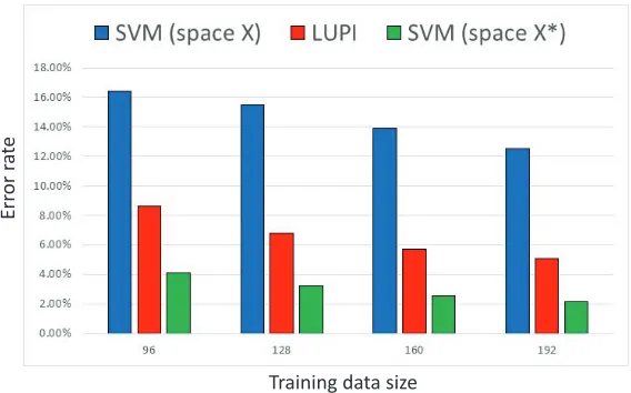
Figure 1: Comparison of SVM and knowledge transfer error rates: video snapshots example.
• SVM with RBF kernel trained on 116 features of spaceX∗;
• SVM with RBF kernel trained 15 original features of space X augmented with 116 knowledge transfer features, each constructed using regressions on the 15-dimensional decision space X (as outlined in subsection 5.2).
Parameters for SVMs with RBF kernel were selected using standard grid search with 6-fold cross validation.
Figure 1 illustrates performance (defined as an overage of error rate) of three algorithms each trained of 50 randomly selected subsets of sizes 64, 96, 128, 160, and 192: SVM in space X, SVM in spaceX∗, and SVM in space with transferred knowledge.
Figure 1 shows that, the larger is the training size, the better is the effect of knowledge transfer. For the largest training size considered in this experiment, the knowledge transfer was capable to recover almost 70% of the error rate gap between the error rates of SVM using only standard features and SVM using privileged features. In this Figure, one also can see that, even in the best case, the error rate using SVM in the space of privileged information is half of that of SVM in the space of transferred knowledge. This gap, probably, can be reduced even further by better selection of the fundamental concepts of knowledge in the space of privileged information and / or by constructing better regression.
5.6 General Remarks about Knowledge Transfer
5.6.1 What Knowledge Does Teacher Transfer?
In previous sections, we linked the knowledge of Intelligent Teacher about the problem of interest in X space to his knowledge about this problem in X∗ space15.
One can give the following general mathematical justification for our model of knowledge transfer. Teacher knows that the goal of Student is to construct a good rule in space X
with one of the functions from the setf(x, α), x∈X, α∈Λ with capacity V CX. Teacher
also knows that there exists a rule of the same quality in spaceX∗ – a rule that belongs to the set f∗(x∗, α∗), x∗ ∈ X∗, α∗ ∈ Λ∗ and that has a much smaller capacity V CX∗. This
knowledge can be defined by the ratio of the capacities
κ= V CX
V CX∗.
The larger is κ, the more knowledge Teacher can transfer to Student; also the larger is κ, the fewer examples will Student need to select a good classification rule.
5.6.2 Learning from Multiple Intelligent Teachers
Model of learning with Intelligent Teachers can be generalized for the situation when Student hasm >1 Intelligent Teachers that produce m training triplets
(xk1, x
k∗
k1, y1), ...,(xk`, x
k∗
k`, y`),
where xkt, k = 1, ..., m, t = 1, ..., ` are elements x of different training data generated by
the same generator P(x) and xkkt∗, k = 1, ..., m, t = 1, ..., ` are elements of the privileged information generated by kth Intelligent Teacher that uses generator Pk(xk∗|x). In this
situation, the method of knowledge transfer described above can be expanded in space X
to include the knowledge delivered by allm Teachers.
5.6.3 Quadratic Kernel
In the method of knowledge transfer, the special role belongs to the quadratic kernel (x1, x2)2. Formally, only two kernels are amenable for simple methods of finding the smallest
number of fundamental elements of knowledge: the linear kernel (x1, x2) and the quadratic
kernel (x1, x2)2.
Indeed, if linear kernel is used, one constructs the separating hyperplane in the space of privileged information X∗
y= (w∗, x∗) +b∗,
where vector of coefficientsw∗also belongs to the spaceX∗, so there is only one fundamental element of knowledge, i.e., the vectorw∗. In this situation, the problem of constructing the regression function y=φ(x) from data
(x1,(w∗, x∗1)), ...,(x`,(w∗, x∗`)) (37)
has, generally speaking, the same level of complexity as the standard problem of pattern recognition in space X using data (35). Therefore, one should not expect performance improvement when transferring the knowledge using (37).
With quadratic kernel, one obtains fewer than dfundamental elements of knowledge in
function intomfragments (a linear combination of which defines the decision rule) and then estimates each of m functions φk(x) separately, using training sets of size `. The idea is
that, in order to estimate a fragment of the knowledge well, one can use a set of functions with a smaller capacity than is needed to estimate the entire function y =f(x), x ∈ X. Here privileged information can improve accuracy of estimation of the desired function.
To our knowledge, there exists only one nonlinear kernel (the quadratic kernel) that leads to an exact solution of the problem of finding the fundamental elements of knowledge. For all other nonlinear kernels, the problems of finding the minimal number of fundamental elements require difficult (heuristic) computational procedures.
6. Conclusions
In this paper, we tried to understand mechanisms of learning that go beyond brute force methods of function estimation. In order to accomplish this, we used the concept of In-telligent Teacher who generates privileged information during training session. We also described two mechanisms that can be used to accelerate the learning process:
1. The mechanism to control Student’s concept of similarity between training examples.
2. The mechanism to transfer knowledge from the space of privileged information to the desired decision rule.
It is quite possible that there exist more mechanisms in Teacher-Student interactions and thus it is important to find them.
The idea of privileged information can be generalized to any statistical inference problem creating non-symmetric (two spaces) approach in statistics.
Teacher-Student interaction constitutes one of the key factors of intelligent behavior and it can be viewed as a basic element in understanding intelligence (for both machines and humans).
Acknowledgments
This material is based upon work partially supported by AFRL and DARPA under contract FA8750-14-C-0008. Any opinions, findings and / or conclusions in this material are those of the authors and do not necessarily reflect the views of AFRL and DARPA.
We thank Professor Cherkassky, Professor Gammerman, and Professor Vovk for their helpful comments on this paper.
References
R. Brachman and H. Levesque.Knowledge Representation and Reasoning. Morgan Kaufman Publishers, San Francisco, CA, 2004.
A. Chervonenkis. Computer Data Analysis (in Russian). Yandex, Moscow, 2013.
L. Devroye, L. Gy¨orfi, and G. Lugosi. A Probabilistic Theory of Pattern Recognition. Ap-plications of mathematics : stochastic modelling and applied probability. Springer, 1996.
L. Gurvits. A note on a scale-sensitive dimension of linear bounded functionals in banach spaces. Theoretical Computer Science, 261(1):81–90, 2001.
G. Kimeldorf and G. Wahba. Some results on tchebycheffian spline functions. Journal of Mathematical Analysis and Applications, 33(1):82–95, 1971.
L. Liang and V. Cherkassky. Connection between SVM+ and multi-task learning. In Proceedings of the International Joint Conference on Neural Networks, IJCNN 2008, part of the IEEE World Congress on Computational Intelligence, WCCI 2008, Hong Kong, China, June 1-6, 2008, pages 2048–2054, 2008.
D. Pechyony, R. Izmailov, A. Vashist, and V. Vapnik. Smo-style algorithms for learning using privileged information. InInternational Conference on Data Mining, pages 235–241, 2010.
B. Ribeiro, C. Silva, N. Chen, A. Vieira, and J. das Neves. Enhanced default risk models with svm+. Expert Systems with Applications, 39(11):10140–10152, 2012.
B. Sch¨olkopf, R. Herbrich, and A. Smola. A generalized representer theorem. InProceedings of the 14th Annual Conference on Computational Learning Theory and and 5th European Conference on Computational Learning Theory, COLT ’01/EuroCOLT ’01, pages 416– 426, London, UK, UK, 2001. Springer-Verlag.
V. Sharmanska, N. Quadrianto, and C. Lampert. Learning to rank using privileged infor-mation. In Computer Vision (ICCV), 2013 IEEE International Conference on, pages 825–832. IEEE, 2013.
V. Vapnik. Estimation of Dependences Based on Empirical Data: Springer Series in Statis-tics (Springer Series in StatisStatis-tics). Springer-Verlag New York, Inc., 1982.
V. Vapnik. The Nature of Statistical Learning Theory. Springer-Verlag New York, Inc., New York, NY, USA, 1995.
V. Vapnik. Statistical Learning Theory. Wiley-Interscience, 1998.
V. Vapnik. Estimation of Dependencies Based on Empirical Data. Springer–Verlag, 2nd edition, 2006.
V. Vapnik and A. Chervonenkis. Theory of Pattern Recognition (in Russian). Nauka, Moscow, 1974.
V. Vapnik and R. Izmailov. Learning with intelligent teacher: Similarity control and knowl-edge transfer. In A. Gammerman, V. Vovk, and H. Papadopoulos, editors, Statistical Learning and Data Sciences, volume 9047 ofLecture Notes in Computer Science, pages 3–32. Springer International Publishing, 2015b.
V. Vapnik and A. Vashist. A new learning paradigm: Learning using privileged information. Neural Networks, 22(5-6):544–557, 2009.