Early Stopping and Non-parametric Regression:
An Optimal Data-dependent Stopping Rule
Garvesh Raskutti [email protected]
Department of Statistics
University of Wisconsin-Madison Madison, WI 53706-1799, USA
Martin J. Wainwright [email protected]
Bin Yu [email protected]
Department of Statistics∗ University of California
Berkeley, CA 94720-1776, USA
Editor:Sara van de Geer
Abstract
Early stopping is a form of regularization based on choosing when to stop running an iterative algorithm. Focusing on non-parametric regression in a reproducing kernel Hilbert space, we analyze the early stopping strategy for a form of gradient-descent applied to the least-squares loss function. We propose a data-dependent stopping rule that does not involve hold-out or cross-validation data, and we prove upper bounds on the squared error of the resulting function estimate, measured in either theL2(P) andL2(Pn) norm. These
upper bounds lead to minimax-optimal rates for various kernel classes, including Sobolev smoothness classes and other forms of reproducing kernel Hilbert spaces. We show through simulation that our stopping rule compares favorably to two other stopping rules, one based on hold-out data and the other based on Stein’s unbiased risk estimate. We also establish a tight connection between our early stopping strategy and the solution path of a kernel ridge regression estimator.
Keywords: early stopping, non-parametric regression, kernel ridge regression, stopping rule, reproducing kernel hilbert space, rademacher complexity, empirical processes
1. Introduction
The phenomenon of overfitting is ubiquitous throughout statistics. It is especially problem-atic in nonparametric problems, where some form of regularization is essential in order to prevent it. In the non-parametric setting, the most classical form of regularization is that of Tikhonov regularization, where a quadratic smoothness penalty is added to the least-squares loss. An alternative and algorithmic approach to regularization is based on early stopping of an iterative algorithm, such as gradient descent applied to the unregularized loss function. The main advantage of early stopping for regularization, as compared to penalized forms, is lower computational complexity.
The idea of early stopping has a fairly lengthy history, dating back to the 1970’s in the context of the Landweber iteration. For instance, see the paper by Strand (1974) as well as the subsequent papers (Anderssen and Prenter, 1981; Wahba, 1987). Early stopping has also been widely used in neural networks (Morgan and Bourlard, 1990), for which stochastic gradient descent is used to estimate the network parameters. Past work has provided intuitive arguments for the benefits of early stopping. Roughly speaking, it is clear that each step of an iterative algorithm will reduce bias but increase variance, so early stopping ensures the variance of the estimator is not too high. However, prior to the 1990s, there had been little theoretical justification for these claims. A more recent line of work has developed a theory for various forms of early stopping, including boosting algorithms (Bartlett and Traskin, 2007; Buhlmann and Yu, 2003; Freund and Schapire, 1997; Jiang, 2004; Mason et al., 1999; Yao et al., 2007; Zhang and Yu, 2005), greedy methods (Barron et al., 2008), gradient descent over reproducing kernel Hilbert spaces (Caponneto, 2006; Caponetto and Yao, 2006; Vito et al., 2010; Yao et al., 2007), the conjugate gradient algorithm (Blanchard and Kramer, 2010), and the power method for eigenvalue computation (Orecchia and Mahoney, 2011). Most relevant to our work is the paper of Buhlmann and Yu (2003), who derived optimal mean-squared error bounds forL2-boosting with early stopping in the case of fixed design regression. However, these optimal rates are based on an “oracle” stopping rule, one that cannot be computed based on the data. Thus, their work left open the following natural question: is there a data-dependent and easily computable stopping rule that produces a minimax-optimal estimator?
The main contribution of this paper is to answer this question in the affirmative for a certain class of non-parametric regression problems, in which the underlying regression function belongs to a reproducing kernel Hilbert space (RKHS). In this setting, a stan-dard estimator is the method of kernel ridge regression (Wahba, 1990), which minimizes a weighted sum of the least-squares loss with a squared Hilbert norm penalty as a regularizer. Instead of a penalized form of regression, we analyze early stopping of an iterative update that is equivalent to gradient descent on the least-squares loss in an appropriately chosen coordinate system. By analyzing the mean-squared error of our iterative update, we derive a data-dependent stopping rule that provides the optimal trade-off between the estimated bias and variance at each iteration. In particular, our stopping rule is based on the first time that a running sum of step-sizes aftert steps increases above the critical trade-off between bias and variance. For Sobolev spaces and other types of kernel classes, we show that the function estimate obtained by this stopping rule achieves minimax-optimal estimation rates in both the empirical and generalization norms. Importantly, our stopping rule does not require the use of cross-validation or hold-out data.
In more detail, our first main result (Theorem 1) provides bounds on the squared pre-diction error for all iterates prior to the stopping time, and a lower bound on the squared error for all iterations after the stopping time. These bounds are applicable to the case of fixed design, where as our second main result (Theorem 2) provides similar types of upper bounds for randomly sampled covariates. These bounds are stated in terms of the squared L2(P) norm or generalization error, as opposed to the in-sample prediction error, or
equiv-alently, the L2(Pn) seminorm defined by the data. Both of these theorems apply to any
our stopping rule yields a function estimate that achieves the minimax optimal rate (up to a constant pre-factor), so that the bounds from our analysis are essentially unimprov-able. Our proof is based on a combination of analytic techniques (Buhlmann and Yu, 2003) with techniques from empirical process theory (van de Geer, 2000). We complement these theoretical results with simulation studies that compare its performance to other rules, in particular a method using hold-out data to estimate the risk, as well as a second method based on Stein’s Unbiased Risk Estimate (SURE). In our experiments for first-order Sobolev kernels, we find that our stopping rule performs favorably compared to these alternatives, especially as the sample size grows. In Section 3.4, we provide an explicit link between our early stopping strategy and the kernel ridge regression estimator.
2. Background and Problem Formulation
We begin by introducing some background on non-parametric regression and reproducing kernel Hilbert spaces, before turning to a precise formulation of the problem studied in this paper.
2.1 Non-parametric Regression and Kernel Classes
Suppose that our goal is to use a covariateX∈ X to predict a real-valued responseY ∈R. We do so by using a function f :X → R, where the value f(x) represents our prediction of Y based on the realization X =x. In terms of mean-squared error, the optimal choice is the regression function defined by f∗(x) : =E[Y |x]. In the problem of non-parametric
regression with random design, we observe n samples of the form {(xi, yi), i= 1, . . . , n},
each drawn independently from some joint distribution on the Cartesian product X ×R, and our goal is to estimate the regression functionf∗. Equivalently, we observe samples of the form
yi =f∗(xi) +wi, fori= 1,2, . . . , n,
where wi : = yi−f∗(xi) are independent zero-mean noise random variables. Throughout
this paper, we assume that the random variables wi are sub-Gaussian with parameter σ,
meaning that
E[etwi]≤et
2σ2/2
for all t∈R.
For instance, this sub-Gaussian condition is satisfied for normal variateswi ∼N(0, σ2), but
it also holds for various non-Gaussian random variables. Parts of our analysis also apply to the fixed design setting, in which we condition on a particular realization{xi}ni=1 of the covariates.
In order to estimate the regression function, we make use of the machinery of reproducing kernel Hilbert spaces (Aronszajn, 1950; Wahba, 1990; Gu and Zhu, 2001). UsingPto denote
the marginal distribution of the covariates, we consider a Hilbert spaceH ⊂L2(P), meaning
a family of functionsg:X →R, withkgkL2(
P)<∞, and an associated inner producth·,·iH
f(x) =hf, K(·, x)iH for allf ∈ H. Any such kernel function must be positive semidefinite.
Moreover, under suitable regularity conditions, Mercer’s theorem (1909) guarantees that the kernel has an eigen-expansion of the form
K(x, x0) = ∞ X
k=1
λkφk(x)φk(x0),
where λ1 ≥ λ2 ≥ λ3 ≥ . . . ≥ 0 are a non-negative sequence of eigenvalues, and {φk}∞k=1 are the associated eigenfunctions, taken to be orthonormal inL2(P). The decay rate of the
eigenvalues will play a crucial role in our analysis.
Since the eigenfunctions {φk}∞k=1 form an orthonormal basis, any function f ∈ H has an expansion of the form f(x) =P∞
k=1
√
λkakφk(x), where for all k such that λk >0, the
coefficients
ak: =
1
√
λk
hf, φkiL2(
P)=
Z
X
f(x)φk(x)dP(x)
are rescaled versions of the generalized Fourier coefficients.1 Associated with any two functions inH—wheref =P∞
k=1
√
λkakφk andg=P∞k=1
√
λkbkφk—are two distinct inner
products. The first is the usual inner product in the space L2(P)—namely, hf, giL2(
P): =
R
Xf(x)g(x)dP(x). By Parseval’s theorem, it has an equivalent representation
in terms of the rescaled expansion coefficients and kernel eigenvalues—that is,
hf, giL2(
P)=
∞ X
k=1
λkakbk.
The second inner product, denoted by hf, giH, is the one that defines the Hilbert space; it
can be written in terms of the rescaled expansion coefficients as
hf, giH= ∞ X
k=1 akbk.
Using this definition, the unit ball for the Hilbert space H with eigenvalues {λk}∞k=1 and
eigenfunctions {φk}∞k=1 takes the form
BH(1) : =f = ∞ X
k=1
p
λkbkφk for some ∞ X
k=1
b2k≤1 .
The class of reproducing kernel Hilbert spaces contains many interesting classes that are widely used in practice, including polynomials of degreed, Sobolev spaces of varying smooth-ness, and Gaussian kernels. For more background and examples on reproducing kernel Hilbert spaces, we refer the reader to various standard references (Aronszajn, 1950; Saitoh, 1988; Sch¨olkopf and Smola, 2002; Wahba, 1990; Weinert, 1982).
Throughout this paper, we assume that any function f in the unit ball of the Hilbert space is uniformly bounded, meaning that there is some constantB <∞ such that
kfk∞: = sup x∈X
|f(x)| ≤B for allf ∈BH(1). (1)
This boundedness condition (1) is satisfied for any RKHS with a kernel such that supx∈XK(x, x) ≤ B. Kernels of this type include the Gaussian and Laplacian kernels,
the kernels underlying Sobolev and other spline classes, as well as as well as any trace class kernel with trignometric eigenfunctions. The boundedness condition (1) is quite stan-dard in non-asymptotic analysis of non-parametric regression procedures (e.g., van de Geer, 2000). We study non-parametric regression when the unknown function f∗ is viewed as fixed, meaning that no prior is imposed on the function space.
2.2 Gradient Update Equation
We now turn to the form of the gradient update that we study in this paper. Given the samples{(xi, yi)}ni=1, consider minimizing the least-squares loss function
L(f) : = 1 2n
n X
i=1
yi−f(xi) 2
over some subset of the Hilbert space H. By the representer theorem (Kimeldorf and Wahba, 1971), it suffices to restrict attention to functions f belonging to the span of the kernel functions defined on the data points—namely, the span of {K(·, xi), i= 1, . . . , n}.
Accordingly, we adopt the parameterization
f(·) = √1
n
n X
i=1
ωiK(·, xi), (2)
for some coefficient vector ω ∈ Rn. Here the rescaling by 1/√n is for later theoretical
convenience.
Our gradient descent procedure is based on a parameterization of the least-squares loss that involves theempirical kernel matrix K ∈Rn×n with entries
[K]ij =
1
nK(xi, xj) fori, j= 1,2, . . . , n.
For any positive semidefinite kernel function, this matrix must be positive semidefinite, and so has a unique symmetric square root denoted by√K. By first introducing the convenient shorthandy1n: = y1 y2 · · ·yn
∈Rn, we can write the least-squares loss in the form
L(ω) = 1 2nky
n
1 −
√
nKωk22.
A direct approach would be to perform gradient descent on this form of the least-squares loss. For our purposes, it turns out to be more natural to perform gradient descent in the transformed co-ordinate system θ = √K ω. Some straightforward calculations (see Appendix A for details) yield that the gradient descent algorithm in this new co-ordinate system generates a sequence of vectors {θt}∞t=0 via the recursion
θt+1 =θt−αt
K θt−
1
√
n
√
K yn1
where {αt}∞t=0 is a sequence of positive step sizes (to be chosen by the user). We assume throughout that the gradient descent procedure is initialized withθ0 = 0.
The parameter estimate θt at iteration tdefines a function estimate ft in the following
way. We first compute2 the weight vectorωt =√K−1 θ
t, which then defines the function
estimate ft(·) = √1nPin=1ωtiK(·, xi) as before. In this paper, our goal is to study how
the sequence {ft}∞t=0 evolves as an approximation to the true regression function f∗. We measure the error in two different ways: the L2(Pn) norm
kft−f∗k2n: =
1 n
n X
i=1
ft(xi)−f∗(xi) 2
compares the functions only at the observed design points, whereas theL2(P)-norm kft−f∗k22 : =E
h
ft(X)−f∗(X) 2i
corresponds to the usual mean-squared error.
2.3 Overfitting and Early Stopping
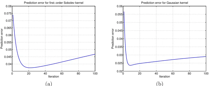
In order to illustrate the phenomenon of interest in this paper, we performed some sim-ulations on a simple problem. In particular, we formed n = 100 i.i.d. observations of the form y = f∗(xi) +wi, where wi ∼ N(0,1), and using the fixed design xi = i/n for
i = 1, . . . , n. We then implemented the gradient descent update (3) with initialization θ0= 0 and constant step sizesαt= 0.25. We performed this experiment with the regression
functionf∗(x) =|x−1/2| −1/2, and two different choices of kernel functions. The kernel
K(x, x0) = min{x, x0}on the unit square [0,1]×[0,1] generates an RKHS of Lipschitz
func-tions, whereas the Gaussian kernel K(x, x0) = exp(−12(x−x0)2) generates a smoother class
of infinitely differentiable functions.
Figure 1 provides plots of the squared prediction error kft−f∗k2n as a function of the
iteration number t. For both kernels, the prediction error decreases fairly rapidly, reaching a minimum before or aroundT ≈20 iterations, before then beginning to increase. As the analysis of this paper will clarify, too many iterations lead to fitting the noise in the data (i.e., the additive perturbationswi), as opposed to the underlying functionf∗. In a nutshell,
the goal of this paper is to quantify precisely the meaning of “too many” iterations, and in a data-dependent and easily computable manner.
3. Main Results and Consequences
In more detail, our main contribution is to formulate a data-dependent stopping rule, mean-ing a mappmean-ing from the data {(xi, yi)}ni=1 to a positive integerTb, such that the two forms
of prediction error kf
b
T −f
∗k
n and kfTb−f∗k2 are minimal. In our formulation of such a
2. If the empirical matrixK is not invertible, then we use the pseudoinverse. Note that it may appear as though a matrix inversion is required to estimate ωt for eacht which is computationally intensive. However, the weightsωtmay be computed directly via the iterationωt+1=ωt−α
tK(ωt− yn
1
√
0 20 40 60 80 100 0.04
0.045 0.05 0.055 0.06 0.065 0.07 0.075 0.08
Iteration
Prediction error
Prediction error for first−order Sobolev kernel
0 20 40 60 80 100
0.02 0.025 0.03 0.035 0.04 0.045 0.05 0.055 0.06
Iteration
Prediction error
Prediction error for Gaussian kernel
(a) (b)
Figure 1: Behavior of gradient descent update (3) with constant step sizeα = 0.25 applied to least-squares loss with n = 100 with equi-distant design points xi = i/n for
i= 1, . . . , n, and regression functionf∗(x) =|x−1/2|−1/2. Each panel gives plots theL2(Pn) errorkft−f∗k2nas a function of the iteration numbert= 1,2, . . . ,100.
(a) For the first-order Sobolev kernelK(x, x0) = min{x, x0}. (b) For the Gaussian
kernelK(x, x0) = exp(−12(x−x0)2).
stopping rule, two quantities play an important role: first, therunning sumof the step sizes
ηt: = t−1
X
τ=0 ατ,
and secondly, the eigenvalues bλ1 ≥ λb2 ≥ · · · ≥ bλn ≥ 0 of the empirical kernel matrix K
previously defined (2.2). The kernel matrix and hence these eigenvalues are computable from the data. We also note that there is a large body of work on fast computation of kernel eigenvalues (e.g., see Drineas and Mahoney, 2005 and references therein).
3.1 Stopping Rules and General Error Bounds
Our stopping rule involves the use of a model complexity measure, familiar from past work on uniform laws over kernel classes (Bartlett et al., 2005; Koltchinskii, 2006; Mendelson, 2002), known as the local empirical Rademacher complexity. For the kernel classes studied in this paper, it takes the form
b
RK(ε) : =
1 n
n X
i=1
minλbi, ε2 1/2
. (4)
solution to the inequality
b
RK(ε)≤ε2/(2eσ). (5) The existence and uniqueness of bεn is guaranteed for any reproducing kernel Hilbert space;
see Appendix D for details. As clarified in our proof, this inequality plays a key role in trading off the bias and variance in a kernel regression estimate.
Our stopping rule is defined in terms of an analogous inequality that involves the running sum ηt=Pt−τ=01 ατ of the step sizes. Throughout this paper, we assume that the step sizes
are chosen to satisfy the following properties:
• Boundedness: 0 ≤ ατ ≤ min{1,1/bλ1}for all τ = 0,1,2, . . .. • Non-increasing: ατ+1 ≤ατ for all τ = 0,1,2, . . ..
• Infinite travel: the running sum ηt=Pτt−=01 ατ diverges ast→+∞.
We refer to any sequence{ατ}∞τ=0that satisfies these conditions as avalid stepsize sequence. We then define the stopping time
b
T : = arg min
t∈N |RbK 1/ √
ηt
>(2eσηt)−1
−1. (6)
As discussed in Appendix D, the integer Tb belongs to the interval [0,∞) and is unique
for any valid stepsize sequence. As will be clarified in our proof, the intuition underlying the stopping rule (6) is that the sum of the step-sizes ηt acts as a tuning parameter that
controls the bias-variance tradeoff. The minimizing value is specified by a fixed point of the local Rademacher complexity, in a manner analogous to certain calculations in empirical process theory (van de Geer, 2000; Mendelson, 2002). The stated choice ofTboptimizes the
bias-variance trade-off.
The following result applies to any sequence {ft}∞t=0 of function estimates generated by the gradient iteration (3) with a valid stepsize sequence.
Theorem 1 Given the stopping timeTbdefined by the rule (6)and critical radiusεbndefined in Equation (5), there are universal positive constants(c1, c2) such that the following events
hold with probability at least1−c1exp(−c2nbε
2
n):
(a) For all iterations t= 1,2, ...,Tb:
kft−f∗k2n ≤
4 e ηt
.
(b) At the iterationTb chosen according to the stopping rule (6), we have
kf
b
T −f
∗k2
n≤12εb
2
n.
(c) Moreover, for allt >Tb,
E[kft−f∗k2n]≥
σ2 4 ηtRb
2
K(η −1/2
3.1.1 Remarks
Although the bounds (a) and (b) are stated as high probability claims, a simple integra-tion argument can be used to show that the expected mean-squared error (over the noise variables, with the design fixed) satisfies a bound of the form
Ekft−f∗k2n
≤ 4
e ηt
for allt≤Tb.
To be clear, note that the critical radius εbn cannot be made arbitrarily small, since it
must satisfy the defining inequality (5). But as will be clarified in corollaries to follow, this critical radius is essentially optimal: we show how the bounds in Theorem 1 lead to minimax-optimal rates for various function classes. The interpretation of Theorem 1 is as follows: if the sum of the step-sizesηtremains below the threshold defined by (6), applying
the gradient update (3) reduces the prediction error. Moreover, note that for Hilbert spaces with a larger kernel complexity, the stopping timeTb is smaller, since fitting functions in a
larger class incurs a greater risk of overfitting.
Finally, the lower bound (c) shows that for large t, running the iterative algorithm beyond the optimal stopping point leads to inconsistent estimators for infinite rank kernels. More concretely, let us suppose that bλi >0 for all 1≤i≤n. In this case, we have
ηtRb2K(η −1/2
t ) =
1 n
n X
i=1
min(ˆλiηt,1),
which converges to 1 ast→. Consequently, part (c) implies that lim inft→∞E[kft−f∗k2n]≥ σ2
4 ast→ ∞, thereby showing the inconsistency of the method.
The statement of Theorem 1 is for the case of fixed design points {xi}ni=1, so that the probability is taken only over the sub-Gaussian noise variables{wi}ni=1In the case of random
design pointxi ∼P i.i.d. , we can also provide bounds on generalization error in the form
theL2(P)-normkft−f∗k2. In this setting, for the purposes of comparing to minimax lower
bounds, it is also useful to state some results in terms of the population analog of the local empirical Rademacher complexity (4), namely the quantity
RK(ε) : =
1 n
∞ X
j=1
minλj, ε2 1/2
, (7)
where λj correspond to the eigenvalues of the population kernel K defined in (3). Using
this complexity measure, we define thecritical population rate εnto be the smallest positive
solution to the inequality
40RK(ε)≤ ε
2
σ. (8)
(Our choice of the pre-factor 40 is for later theoretical convenience.) In contrast to the critical empirical rate εbn, this quantity is not data-dependent, since it is specified by the
Theorem 2 (Random design) Suppose that in addition to the conditions of Theorem 1, the design variables{xi}ni=1 are sampled i.i.d. according toPand that the population critical
radiusεnsatisfies inequality (8). Then there are universal constantscj, j = 1,2,3such that
kf
b
T −f
∗k2
2 ≤c3ε2n with probability at least 1−c1exp(−c2nε2n).
Theorems 1 and 2 are general results that apply to any reproducing kernel Hilbert space. Their proofs involve combination of direct analysis of our iterative update (3), combined with techniques from empirical process theory and concentration of measure (van de Geer, 2000; Ledoux, 2001); see Section 4 for the details.
It is worthwhile to compare with the past work of Buhlmann and Yu (2003) (hereafter BY), who also provide some theory for gradient descent, referred to asL2-boosting in their paper, but focusing exclusively on the fixed design case. Our theory applies to random as well as fixed design, and a broader set of stepsize choices. The most significant difference between Theorem 1 in our paper and Theorem 3 of BY is that we provide a data-dependent stopping rule, whereas their analysis does not lead to a stopping rule that can be computed from the data.
3.2 Consequences for Specific Kernel Classes
Let us now illustrate some consequences of our general theory for special choices of kernels that are of interest in practice.
3.2.1 Kernels with Polynomial Eigendecay
We begin with the class of RKHSs whose eigenvalues satisfy apolynomial decay condition, meaning that
λk ≤C
1 k
2β
for someβ >1/2 and constant C. (9)
Among other examples, this type of scaling covers various types of Sobolev spaces, consisting of functions withβ derivatives (Birman and Solomjak, 1967; Gu, 2002). As a very special case, the first-order Sobolev kernel K(x, x0) = min{x, x0} on the unit square [0,1]×[0,1]
generates an RKHS of functions that are differentiable almost everywhere, given by
H: =f : [0,1]→R| f(0) = 0,
Z 1
0
(f0(x))2dx <∞ , (10) For the uniform measure on [0,1], this class exhibits polynomial eigendecay (9) withβ = 1. For any class that satisfies the polynomial decay condition, we have the following corollary:
Corollary 3 Suppose that in addition to the assumptions of Theorem 2, the kernel class H satisfies the polynomial eigenvalue decay (9)for some parameterβ >1/2. Then there is a universal constantc5 such that
EkfTb−f∗k22]≤c5 σ2
n
2β2β+1
Moreover, if λk ≥c(1/k)2β for allk= 1,2, . . ., then
Ekft−f∗k22
≥ 1
4min
1, σ2(ηt)
1 2β
n for all iterations t= 1,2, . . ..
The proof, provided in Section 4.3, involves showing that the population critical rate (7)
is of the order O(n−
2β
2β+1). By known results on non-parametric regression (Stone, 1985;
Yang and Barron, 1999), the error bound (11) is minimax-optimal.
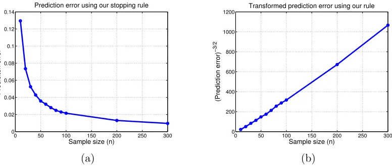
In the special case of the first-order spline family (10), Corollary 3 guarantees that
E[kfTb−f ∗k2
2] -σ2
n
2/3
. (12)
In order to test the accuracy of this prediction, we performed the following set of simulations. First, we generated samples from the observation model
yi=f∗(xi) +wi, fori= 1,2, . . . , n, (13)
where xi = i/n, and wi ∼ N(0, σ2) are i.i.d. noise terms. We present results for the
function f∗(x) = |x−1/2| −1/2, a piecewise linear function belonging to the first-order Sobelev class. For all our experiments, the noise variance σ2 was set to one, but so as to have a data-dependent method, this knowledge was not provided to the estimator. There is a large body of work on estimating the noise variance σ2 in non-parametric regression. For our simulations, we use a simple method due to Hall and Marron (1990). They proved that their estimator is ratio consistent, which is sufficient for our purposes.
For a range of sample sizes n between 10 and 300, we performed the updates (3) with constant stepsizeα = 0.25, stopping at the specified time T. For each sample size, we per-b
formed 10,000 independent trials, and averaged the resulting prediction errors. In panel (a) of Figure 2, we plot the mean-squared error versus the sample size, which shows consistency of the method. The bound (12) makes a more specific prediction: the mean-squared error raised to the power−3/2 should scale linearly with the sample size. As shown in panel (b) of Figure 2, the simulation results do indeed reveal this predicted linear relationship. We also performed the same experiments for the case of randomly drawn designs xi ∼ Unif(0,1).
In this case, we observed similar results, but with more trials required to average out the additional randomness in the design.
3.2.2 Finite Rank Kernels
We now turn to the class of RKHSs based on finite-rank kernels, meaning that there is some finite integerm <∞ such that λj = 0 for all j≥m+ 1. For instance, the kernel function K(x, x0) = (1 +xx0)2 is a finite rank kernel with m= 2, and it generates the RKHS of all
quadratic functions. More generally, for any integerd≥2, the kernel K(x, x0) = (1 +xx0)d
generates the RKHS of all polynomials with degree at mostd. For any such kernel, we have the following corollary:
Corollary 4 If, in addition to the conditions of Theorem 2, the kernel has finite rank m, then
Ekfb b
T −f
∗k2 2
0 50 100 150 200 250 300 0
0.02 0.04 0.06 0.08 0.1 0.12 0.14
Sample size (n)
Prediciton error
Prediction error using our stopping rule
0 50 100 150 200 250 300 0
200 400 600 800 1000 1200
Sample size (n)
(Prediction error)
−3/2
Transformed prediction error using our rule
(a) (b)
Figure 2: Prediction error obtained from the stopping rule (6) applied to a regression model withnsamples of the form f∗(xi) +wi at equidistant design pointsxi =i/nfor
i= 0,1, . . .99, and i.i.d. Gaussian noisewi ∼N(0,1). For these simulations, the
true regression function is given byf∗(x) =|x−1 2| −
1
2. (a) Mean-squared error (MSE) using the stopping rule (6) versus the sample sizen. Each point is based on 10,000 independent realizations of the noise variables {wi}ni=1. (b) Plots of the quantity M SE−3/2 versus sample size n. As predicted by the theory, this form of plotting yields a straight line.
For any rankm-kernel, the rate mn is minimax optimal in terms of squaredL2(P) error; this
fact follows as a consequence of more general lower bounds due to Raskutti et al. (2012).
3.3 Comparison with Other Stopping Rules
In this section, we provide a comparison of our stopping rule to two other stopping rules, as well as a oracle method that involves knowledge of f∗, and so cannot be computed in practice.
3.3.1 Hold-out Method
We begin by comparing to a simple hold-out method that performs gradient descent using 50% of the data, and uses the other 50% of the data to estimate the risk. In more detail, assuming that the sample size is even for simplicity, we split the full data set{xi}ni=1into two equally sized subsetsStrandSte. The data indexed by the training setStris used to estimate
the function ftr,t using the gradient descent update (3). At each iteration t = 0,1,2, . . .,
the data indexed bySte is used to estimate the risk viaRHO(ft) = n1
P
i∈Ste yi−ftr,t(xi)
2
, which defines the stopping rule
b
THO: = arg min
t∈N |RHO(ftr,t+1)> RHO(ftr,t)
A line of past work (Yao et al., 2007; Bauer et al., 2007; Caponneto, 2006; Caponetto and Yao, 2006, 2010; Vito et al., 2010) has analyzed stopping rules based on this type of hold-out rule. For instance, Caponneto (2006) analyzes a hold-out method, and shows that it yields rates that are optimal for Sobolev spaces withβ≤1 but not in general. A major drawback of using a hold-out rule is that it “wastes” a constant fraction of the data, thereby leading to inflated mean-squared error.
3.3.2 SURE Method
Alternatively, we can use Stein’s Unbiased Risk estimate (SURE) to define another stopping rule. Gradient descent is based on the shrinkage matrix ˜St =
Qt−1
τ=0(I−ατK). Based on
this fact, it can be shown that the SURE estimator (Stein, 1981) takes the form
RSU(ft) =
1 n{nσ
2+ (yn
1)T( ˜St)2y1n−2σ2trace( ˜St)}.
This risk estimate can be used to define the associated stopping rule
b
TSU : = arg min
t∈N |RSU(ft+1)> RSU(ft)
−1. (15)
In contrast with hold-out, the SURE stopping rule (15) makes use of all the data. However, we are not aware of any theoretical guarantees for early stopping based on the SURE rule. For any valid sequence of stepsizes, it can be shown that both stopping rules (14) and (15) define a unique stopping time. Note that our stopping rule Tb based on (6) requires
estimation of both the empirical eigenvalues, and the noise variance σ2. In contrast, the SURE-based rule requires estimation of σ2 but not the empirical eigenvalues, whereas the hold-out rule requires no parameters to be estimated, but a percentage of the data is used to estimate the risk.
3.3.3 Oracle Method
As a third point of reference, we also plot the mean-squared error for an “oracle” method. It is allowed to base its stopping time on the exact in-sample prediction error ROR(ft) = kft−f∗k2n, which defines the oracle stopping rule
b
TOR : = arg min
t∈N |ROR(ft+1)> ROR(ft)
−1. (16)
Note that this stopping rule is not computable from the data, since it assumes exact knowl-edge of the functionf∗ that we are trying to estimate.
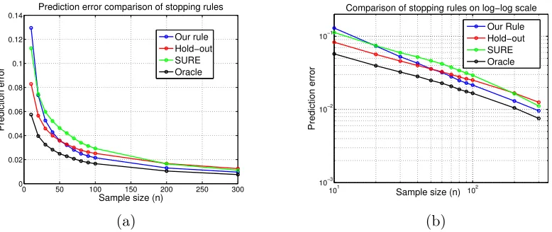
In order to compare our stopping rule (6) with these alternatives, we generated i.i.d. samples from the previously described model (see Equation (13) and the following discus-sion). We varied the sample sizenfrom 10 to 300, and for each sample size, we performed M = 10,000 independent trials (randomizations of the noise variables {wi}ni=1), and com-puted the average of squared prediction error over these M trials.
0 50 100 150 200 250 300 0
0.02 0.04 0.06 0.08 0.1 0.12 0.14
Sample size (n)
Prediction error
Prediction error comparison of stopping rules
Our rule Hold−out SURE Oracle
101
102
10−3
10−2
10−1
Sample size (n)
Prediction error
Comparison of stopping rules on log−log scale
Our Rule Hold−out SURE Oracle
(a) (b)
Figure 3: Illustration of the performance of different stopping rules for kernel gradient de-scent with the kernel K(x, x) = min{|x|,|x0|} and noisy samples of the function
f∗(x) =|x−1 2| −
1
2. In each case, we applied the gradient update (3) with con-stant stepsizesαt= 1 for allt. Each curve corresponds to the mean-squared error,
estimated by averaging over M = 10,000 independent trials, versus the sample size forn∈ {10,20,30,40,50,60,70,80,90,100,200,300}. Each panel shows MSE curves for four different stopping rules: (i) the stopping rule (6); (ii) holding out 50% of the data and using (14); (iii) the SURE stopping rule (15); and (iv) the oracle stopping rule (14). (a) MSE versus sample size on a standard scale. (b) MSE versus sample size on a log-log scale.
same curves in terms of logarithm of mean-squared error. Our proposed rule exhibits better performance than the hold-out and SURE-based rules for sample sizesnlarger than 50. On the flip side, since the construction of our stopping rule is based on the assumption thatf∗ belongs to a known RKHS, it is unclear how robust it would be to model mis-specification. In contrast, the hold-out and SURE-based stopping rules are generic methods, not based directly on the RKHS structure, so might be more robust to model mis-specification. Thus, one interesting direction is to explore the robustness of our stopping rule. On the theoret-ical front, it would be interesting to determine whether the hold-out and/or SURE-based stopping rules can be proven to achieve minimax optimal rates for general kernels, as we have established for our stopping rule.
3.4 Connections to Kernel Ridge Regression
We conclude by presenting an interesting link between our early stopping procedure and kernel ridge regression. The kernel ridge regression (KRR) estimate is defined as
b
fν : = arg min f∈H
1
2n
n X
i=1
(yi−f(xi))2+
1 2νkfk
2
whereν is the (inverse) regularization parameter. For any ν <∞, the objective is strongly convex, so that the KRR solution is unique.
Friedman and Popescu (2004) observed through simulations that the regularization paths for early stopping of gradient descent and ridge regression are similar, but did not provide any theoretical explanation of this fact. As an illustration of this empirical phe-nomenon, Figure 4 compares the prediction errorkfbν −f∗k2n of the kernel ridge regression
estimate over the interval ν ∈[1,100] versus that of the gradient update (3) over the first 100 iterations. Note that the curves, while not identical, are qualitatively very similar.
0 20 40 60 80 100 0.05
0.1 0.15 0.2 0.25 0.3
Inverse penalty parameter
Prediction error
Prediction error for first−order Sobolev kernel
Kernel ridge Gradient
0 20 40 60 80 100
0 0.05 0.1 0.15 0.2 0.25
Inverse penalty parameter
Prediction error
Prediction error for first−order Sobolev kernel
Kernel ridge Gradient
(a) (b)
Figure 4: Comparison of the prediction error of the path of kernel ridge regression esti-mates (17) obtained by varyingν ∈[1,100] to those of the gradient updates (3) over 100 iterations with constant step size. All simulations were performed with the kernelK(x, x0) = min{|x|,|x0|}based onn= 100 samples at the design points
xi =i/nwithf∗(x) =|x−12| −12. (a) Noise varianceσ2 = 1. (b) Noise variance
σ2 = 2.
From past theoretical work (van de Geer, 2000; Mendelson, 2002), kernel ridge regression with the appropriate setting of the penalty parameter ν is known to achieve minimax-optimal error for various kernel classes. These classes include the Sobolev and finite-rank kernels for which we have previously established that our stopping rule (6) yields optimal rates. In this section, we provide a theoretical basis for these connections. More precisely, we prove that if the inverse penalty parameter ν is chosen using the same criterion as our stopping rule, then the prediction error satisfies the same type of bounds, withν now playing the role of the running sum ηt.
Define ν >b 0 to be the smallest positive solution to the inequality
4σν−1
<RbK(1/ √
ν
. (18)
Proposition 5 Consider the kernel ridge regression estimator (17)applied toni.i.d. sam-ples{(xi, yi)}withσ-sub Gaussian noise. Then there are universal constants(c1, c2, c3)such that with probability at least 1−c1exp(−c2nεb
2
n):
(a) For all 0< ν ≤bν, we have
kfbν−f∗k2n≤
2 ν
(b) With bν chosen according to the rule (18), we have
kfb b
ν−f∗k2n≤c3bε
2
n.
(c) Moreover, for allν >νb, we have
E[kfbν −f∗k2n]≥
σ2 4 νRb
2
K(ν −1/2).
Note that apart from a slightly different leading constant, the upper bound (a) is
iden-tical to the upper bound in Theorem 1 part (a). The only difference is that the inverse
regularization parameter ν replaces the running sum ηt=Pt−τ=01 ατ. Similarly, part (b) of
Proposition 5 guarantees that the kernel ridge regression (17) has prediction error that is upper bounded by the empirical critical rate εb
2
n, as in part (b) of Theorem 1. Let us
em-phasize that bounds of this type on kernel ridge regression have been derived in past work (Mendelson, 2002; Zhang, 2005; van de Geer, 2000). The novelty here is that the structure of our result reveals the intimate connection to early stopping, and in fact, the proofs follow a parallel thread.
In conjunction, Proposition 5 and Theorem 1 provide a theoretical explanation for why, as shown in Figure 4, the paths of the gradient descent update (3) and kernel ridge re-gression estimate (17) are so similar. However, it is important to emphasize that from a computational point of view, early stopping has certain advantages over kernel ridge re-gression. In general, solving a quadratic program of the form (17) requires on the order of O(n3) basic operations, and this must be done repeatedly for each new choice of ν. On the other hand, by its very construction, the iterates of the gradient algorithm correspond to the desired path of solutions, and each gradient update involves multiplication by the kernel matrix, incurringO(n2) operations.
4. Proofs
We now turn to the proofs of our main results. The main steps in each proof are provided in the main text, with some of the more technical results deferred to the appendix.
4.1 Proof of Theorem 1
In order to derive upper bounds on the L2(Pn)-error in Theorem 1, we first rewrite the
gradient update (3) in an alternative form. For each iterationt= 0,1,2, . . ., let us introduce the shorthand
ft(xn1) : =
ft(x1) ft(x2) · · · ft(xn)
corresponding to the n-vector obtained by evaluating the function ft at all design points, and the short-hand
w: =w1, w2, ..., wn
∈Rn,
corresponding to the vector of zero mean sub-Gaussian noise random variables. From Equation (2), we have the relation
ft(xn1) = √1
nK ω
t = √1
n
√
K θt.
Consequently, by multiplying both sides of the gradient update (3) by √K, we find that the sequence{ft(xn1)}∞t=0 evolves according to the recursion
ft+1(xn1) =ft(xn1)−αtK(ft(xn1)−y1n) =
In×n−αtK
ft(xn1) +αtK yn1. (19) Since θ0 = 0, the sequence is initialized with f0(xn1) = 0. The recursion (19) lies at the heart of our analysis.
Letting r = rank(K), the empirical kernel matrix has the eigendecomposition K = UΛUT, where U ∈Rn×n is an orthonormal matrix (satisfyingU UT =UTU =In×n) and
Λ : = diag(λ1,b λ2, . . . ,b λbr,0,0,· · · ,0)
is the diagonal matrix of eigenvalues, augmented withn−r zero eigenvalues as needed. We then define a sequence of diagonalshrinkage matrices St as follows:
St: =
t−1
Y
τ=0
(In×n−ατΛ)∈Rn×n.
The matrix St indicates the extent of shrinkage towards the origin; since 0 ≤ αt ≤
min{1,1/λb1}for all iterationst, in the positive semodefinite ordering, we have the sandwich
relation
0St+1 StIn×n.
Moreover, the following lemma shows that theL2(Pn)-error at each iteration can be bounded
in terms of the eigendecomposition and these shrinkage matrices:
Lemma 6 (Bias/variance decomposition) At each iteration t= 0,1,2, . . .,
kft−f∗k2n≤
2 n
r X
j=1
(St)2jj[UTf∗(xn1)]2j + 2 n
n X
j=r+1
[UTf∗(xn1)]2j
| {z }
Squared Bias Bt2
+2 n
r X
j=1
(1−Sjjt )2[UTw]2j
| {z }
Variance Vt
.
(20)
See Appendix B.1 for the proof of this intermediate claim.
In order to complete the proof of the upper bound in Theorem 1, our next step is to obtain high probability upper bounds on these two terms. We summarize our conclusions in an additional lemma, and use it to complete the proof of Theorem 1(a) before returning to prove it.
Lemma 7 (Bounds on the bias and variance) For all iterationst= 1,2, . . ., the squared bias is upper bounded as
Bt2 ≤ 1
e ηt
, (21)
Moreover, there is a universal constant c1 >0 such that, for any iterationt= 1,2, . . . ,Tb,
Vt ≤ 5σ2ηtR2K 1/ √
ηt
(22)
with probability at least 1−exp −c1nεb
2
n
. Moreover we haveE[Vt]≥ σ
2
4 ηtR 2 K 1/ √ ηt .
We can now complete the proof of Theorem 1(a). Conditioned on the event Vt ≤
5σ2ηtR2K 1/ √
ηt
, we have
kft−f∗k2n
(i)
≤Bt2+Vt
(ii)
≤ 1
e ηt
+ 5σ2ηtR2K 1/ √
ηt (iii)
≤ 4
e ηt
,
where inequality (i) follows from (20) in Lemma 6, and inequality (ii) follows from the bounds in Lemma 7 and (iii) follows since t≤Tb. The lower bound (c) follows from (22).
Turning to the proof of part (b), using the upper bound from (a)
kf
b
T −f
∗k2
n≤ 1 e η b T + 5 η b T ≤ 4 eη b T .
Based on the definition of Tb and bεn, we are guaranteed that η1 b T+1
≤εb2n, Moreover, by the non-decreasing nature of our step sizes, we haveα
b
T+1≤αTb, which implies thatηTb+1 ≤2ηTb,
and hence 1 η b T ≤ 2 η b T+1
≤ 2εb2n.
Putting together the pieces establishes the bound claimed in part (b).
It remains to establish the bias and variance bounds stated in Lemma 7, and we do so in the following subsections. The following auxiliary lemma plays a role in both proofs:
Lemma 8 (Properties of shrinkage matrices) For all indices j ∈ {1,2, . . . , r}, the shrinkage matrices St satisfy the bounds
0≤ (St)2jj ≤ 1
2eηtλbj
, and (23)
1
2min{1, ηtλbj} ≤1−S
t
jj ≤min{1, ηtbλj}. (24)
4.1.1 Bounding the Squared Bias
Let us now prove the upper bound (21) on the squared bias. We bound each of the two terms in the definition (20) ofBt2 in term. Applying the upper bound (23) from Lemma 8, we see that
2 n
r X
j=1
(St)2jj[UTf∗(xn1)]2j ≤ 1
e n ηt r X
j=1
[UTf∗(xn1)]2j
b
λj
.
Now consider the linear operator ΦX :`2(N)→Rndefined element-wise via [ΦX]jk =φj(xk).
Similarly, we define a (diagonal) linear operator D:`2(N)→`2(N) with entries [D]jj =λj
and [D]jk = 0 forj6=k. With these definitions, the vectorf(xn1)∈Rncan be expressed in terms of some sequencea∈`2(N) in the form
f(xn1) = ΦXD1/2a.
In terms of these quantities, we can write K = n1ΦXDΦTX. Moreover, as previously noted,
we also have K =UΛUT where Λ = diag{bλ1,λ2, . . . ,b bλn}, and U ∈ Rn×n is orthonormal.
Combining the two representations, we conclude that
ΦX√D1/2
n =UΛ 1/2Ψ∗
,
for some linear operator Ψ : Rn → `2(N) (with adjoint Ψ∗) such that Ψ∗Ψ =In×n. Using
this equality, we have
1 e ηtn
r X
j=1
[UTf∗(X)]2j
b
λj
= 1 e ηtn
r X
j=1
[UTΦXD1/2a]2j b
λj
= 1 e ηt
r X
j=1
[UTUΛ1/2V∗a]2j
b
λj
= 1 e ηt
r X
j=1
b
λj[Ψ∗a]2j b
λj
≤ 1
e ηt
kΨ∗ak22
≤ 1
e ηt
, (25)
Here the final step follows from the fact that Ψ is a unitary operator, so that
kΨ∗ak2
Turning to the second term in the definition (20), we have
n X
j=r+1
[UTf∗(xn1)]2j = 2 n
n X
j=r+1
[UTΦXD1/2a]2j
=
n X
j=r+1
[UTUΛ1/2Ψ∗a]2j
=
n X
j=r+1
[Λ1/2Ψ∗a]2j
= 0, (26)
where the final step uses the fact that Λ1jj/2 = 0 for all j ∈ {r + 1, . . . , n} by construc-tion. Combining the upper bounds (25) and (26) with the definition (20) of Bt2 yields the claim (21).
4.1.2 Controlling the Variance
Let us now prove the bounds (22) on the variance term Vt. (To simplify the proof, we
assume throughout that σ = 1; the general case can be recovered by a simple rescaling argument). By the definition ofVt, we have
Vt=
2 n
r X
j=1
(1−Sjjt )2[UTw]2j = 2
ntrace(U QU
T wwT),
where Q = diag{(1−Sjjt )2, j = 1, . . . , n} is a diagonal matrix. Since E[wwT] ≤In×n by
assumption, we have E[Vt] = n2trace(Q). Using the upper bound in Equation (24) from
Lemma 8, we have
1
ntrace(Q)≤ 1 n
r X
j=1
min{1,(ηtbλj)2} = ηt
RK(1/√ηt)
2
,
where the final equality uses the definition ofRK. Putting together the pieces, we see that
E[Vt]≤2ηt
RK(1/√ηt)
2
.
Similarly, using the lower bound in Equation (24), we can show that
E[Vt]≥
σ2 4 ηt
RK(1/
√
ηt)
2
.
Our next step is to obtain a bound on the two-sided tail probabilityP[|Vt−E[Vt]| ≥δ], for
E[ZiZj]) where {Zi}ni=1 are i.i.d. zero-mean and sub-Gaussian variables (with parameter 1). Wright (1973) proves that there is a constantc such that
P|Q−E[Q]| ≥δ≤exp
−c min δ
|||A|||op,
δ2
|||A|||2 F
for all u >0, (27)
where (|||A|||op,|||A|||F) are (respectively) the operator and Frobenius norms of the matrix A={aij}ni,j=1.
If we apply this result with A = 2nU QUT and Zi = wi, then we have Q = Vt, and
moreover
|||A|||op≤ 2
n, and
|||A|||2F = 4
n2trace(U
TQUTU QUT) = 4
n2 trace(Q 2)≤ 4
n2trace(Q)≤ 4 nηt
RK(1/√ηt)
.
Consequently, the bound (27) implies that
P|Vt−E[Vt]| ≥δ
≤exp −4c n δmin{1, δ
ηtRK(1/ √
ηt) −1
}
.
Since t≤Tb settingδ = 3σ2ηt
RK(1/√ηt)
, the claim (22) follows.
4.2 Proof of Theorem 2
This proof is based on the following two steps:
• first, proving that the error kf
b
T −f
∗k
2 in the L2(P) norm is, with high probability,
close to the error in the L2(Pn) norm, and
• second, showing the empirical critical radius εbn defined in Equation (5) is upper
bounded by the population critical radius εn defined in Equation (8).
Our proof is based on a number of more technical auxiliary lemmas, proved in the appendices. The first lemma provides a high probability bound on the Hilbert norm of the estimate f
b T.
Lemma 9 There exist universal constants c1 andc2 >0 such thatkftkH≤2 for allt≤Tb with probability greater than or equal to 1−c1exp(−c2nεb
2
n).
See Appendix E.1 for the proof of this claim. Our second lemma shows in any bounded RKHS, theL2(
P) andL2(Pn) norms are uniformly close up to the population critical radius
εn over a Hilbert ball of constant radius:
Lemma 10 Consider a Hilbert space such that kgk∞ ≤ B for all g ∈ BH(3). Then there exist universal constants (c1, c2, c3) such that for any t≥εn, we have
|kgk2n− kgk22| ≤ c1t2,
This claim follows from known results on reproducing kernel Hilbert spaces (e.g., Lemma 5.16 in the paper van de Geer, 2000 and Theorem 2.1 in the paper Bartlett et al., 2005). Our final lemma, proved in Appendix E.2, relates the critical empirical radius εbn to the
population radius εn:
Lemma 11 There exist constantsc1 andc2 such thatbεn≤εn holds with probability at least
1−c1exp(−c2nε2n).
With these lemmas in hand, the proof of the theorem is straightforward. First, from Lemma 9, we have kf
b
TkH ≤2 and hence by triangle inequality, kfTb−f ∗k
H≤3 with high
probability as well. Next, applying Lemma 10 witht=εn, we find that
kfTb−f∗k22 ≤ kfTb−f∗k2n+c1ε2n≤c4(bε
2
n+ε2n),
with probability greater than 1−c2exp(−c3nε2n). Finally, applying Lemma 11 yields that the bound kf
b
T −f
∗k2
2≤cε2n holds with the claimed probability.
4.3 Proof of Corollaries
In each case, it suffices to upper bound the generalization rateε2n previously defined.
4.3.1 Proof of Corollary 4
In this case, we have
RK() = √1
n
v u u t
m X
j=1
min{λj, 2} ≤ r
m n
so that ε2n=c0σ2mn.
4.3.2 Proof of Corollary 3
For anyM ≥1, we have
RK() = √1
n
v u u t
∞ X
j=1
min{C j−2β, 2} ≤
r
M n +
r
C n
v u u t
∞ X
j=dMe
j−2β
≤ r
M n +
r
C0
n
s
Z ∞
M
t−2βdt
≤ r
M n +C
00√1
n(1/M)
β−12.
SettingM =−1/β yieldsR
K()≤C
∗1−21β
. Consequently, the critical inequality
RK()≤402/σ is satisfied forεn(σ2/n)
2β
4.4 Proof of Proposition 5
We now turn to the proof of our results on the kernel ridge regression estimate (17). The proof follows a very similar structure to that of Theorem 1. Recall the eigendecomposition K =UΛUT of the empirical kernel matrix, and that we use r to denote its rank. For each ν >0, we define the ridge shrinkage matrix
Rν : = In×n+νΛ−1. (28)
We then have the following analog of Lemma 7 from the proof of Theorem 1:
Lemma 12 (Bias/variance decomposition for kernel ridge regression) For anyν > 0, the prediction error for the estimate fbν is bounded as
kfbν −f∗k2n≤
2 n
r X
j=1
[Rν]2jj[UTf∗(xn1)]2j + 2 n
n X
j=r+1
[UTf∗(xn1)]2j+ 2 n
r X
j=1
1−Rνjj2
[UTw]2j.
Note that Lemma 12 is identical to Lemma 7 with the shrinkage matrices St replaced by their analogues Rν. See Appendix C.1 for the proof of this claim.
Our next step is to show that the diagonal elements of the shrinkage matrices Rν are bounded:
Lemma 13 (Properties of kernel ridge shrinkage) For all indices j ∈ {1,2, . . . , r}, the diagonal entries Rν satisfy the bounds
0 ≤ (Rνjj)2 ≤ 1
4νbλj
, and (29)
1 2min
1, νbλj ≤ 1−Rνjj ≤ min
1, νbλj .
Note that this is the analog of Lemma 8 from Theorem 1, albeit with the constant 14 in the bound (29) instead of 21e. See Appendix C.2 for the proof of this claim. With these lemmas in place, the remainder of the proof follows as in the proof of Theorem 1.
5. Discussion
In this paper, we have analyzed the early stopping strategy as applied to gradient descent on the non-parametric least squares loss. Our main contribution was to propose an easily computable and data-dependent stopping rule, and to provide upper bounds on the empir-icalL2(Pn) error (Theorem 1) and generlizationL2(P) error (Theorem 2). We demonstrate
in Corollaries 3 and 4 that our stopping rule yields minimax optimal rates for both low rank kernel classes and Sobolev spaces. Our simulation results confirm that our stopping rule yields theoretically optimal rates of convergence for Lipschitz kernels, and performs fa-vorably in comparison to stopping rules based on hold-out data and Stein’s Unbiased Risk Estimate. We also showed that early stopping with sum of step-sizes ηt = Pt−k=01 αk has
Our analysis and stopping rule may be improved and extended in a number of ways. First, it would interesting to see how our stopping rule can be adapted to mis-specified models. As specified, our method relies on computation of the eigenvalues of the kernel matrix. A stopping rule based on approximate eigenvalue computations, for instance via some form of sub-sampling (Drineas and Mahoney, 2005), would be interesting to study as well.
Acknowledgments
This work was partially supported by NSF grant DMS-1107000 to MJW and BY. In addi-tion, BY was partially supported by the NSF grant SES-0835531 (CDI), ARO-W911NF-11-1-0114 and the Center for Science of Information (CSoI), an US NSF Science and Technol-ogy Center, under grant agreement CCF-0939370, and MJW was also partially supported ONR MURI grant N00014-11-1-086. During this work, GR received partial support from a Berkeley Graduate Fellowship.
Appendix A. Derivation of Gradient Descent Updates
In this appendix, we provide the details of how the gradient descent updates (3) are obtained. In terms of the transformed vector θ=√K ω, the least-squares objective takes the form
e
L(θ) : = 1 2nky
n
1 −
√
n
√
K θk22 = 1 2nky
n
1k22− 1
√
nhy
n
1,
√
K θi+1 2(θ)
TKθ.
Given a sequence{αt}∞t=0, the gradient descent algorithm operates via the recursionθt+1= θt−αt∇Le(θt). Taking the gradient ofLeyields
∇Le(θ) =K θ−
1
√
n
√
K y1n.
Substituting into the gradient descent update yields the claim (3).
Appendix B. Auxiliary Lemmas for Theorem 1
In this appendix, we collect together the proofs of the lemmas for Theorem 1.
B.1 Proof of Lemma 6
We prove this lemma by analyzing the gradient descent iteration in an alternative co-ordinate system. In particular, given a vector ft(xn1) ∈ Rn and the SVD K = UΛUT of
the empirical kernel matrix, we define the vectorγt= √1
nU
Tft(xn
1). In this new-coordinate system, our goal is to estimate the vector γ∗ = √1
nU
Tf∗(xn
1). Recalling the alternative form (19) of the gradient recursion, some simple algebra yields that the sequence {γt}∞t=0
evolves as
γt+1 =γt+αtΛ
˜ w
√
n −αtΛ(γ
t−γ∗
where ˜w : =UTw is a rotated noise vector. Since γ0 = 0, unwrapping this recursion then yields γt−γ∗ = I −St√w˜
n −S
tγ∗, where we have made use of the previously defined
shrinkage matricesSt. Using the inequality ka+bk2
2 ≤2(kak22+kbk22), we find that
kγt−γ∗k22 ≤ 2
nk(I−S
t) ˜wk2
2+ 2kStγ∗k22 = 2
nk(I−S
t) ˜wk2 2+ 2
r X
j=1
[St]2jj(γjj∗ )2+ 2
n X
j=r+1 (γjj∗ )2.
where the equality uses the fact that λbj = 0 for all j ∈ {r + 1, . . . , n}. Finally, the
orthogonality of U implies that kγt−γ∗k2
2 = n1kf t(xn
1)−f∗(xn1)k22, from which the upper bound (20) follows.
B.2 Proof of Lemma 8
Using the definition of Stand the elementary inequality 1−u≤exp(−u), we have
[St]2jj =
t−1
Y
τ=0
(1−ατbλj)
2
≤exp(−2ηtbλj)
(i)
≤ 1
2eηtbλj
,
where inequality (i) follows from the fact that sup
u∈R
uexp(−u) = 1/e.
Turning to the second set of inequalities, we have 1−[St]jj = 1−Qt−τ=01 (1−ατbλj). By
induction, it can be shown that
1−[St]jj ≤1−max{0,1−ηtbλj}= min{1, ηtbλj}.
As for the remaining claim, we have
1− t−1
Y
τ=0
(1−ατλbj)
(i)
≥1−exp(−ηtλbi)
(ii)
≥ 1−(1 +ηtλbi)−1
= ηtλbi 1 +ηtλbi
≥ 1
2min{1, ηtλbi},
where step (i) follows from the inequality 1−u ≤exp(−u); and step (ii) follows from the inequality exp(−u)≤(1 +u)−1, valid foru >0.
Appendix C. Auxiliary Results for Proposition 5
C.1 Proof of Lemma 12
By definition of the KRR estimate, we have
K+1νI
fν(xn1) =Ky1n. Consequently, some straightforward algebra yields the relation
UTfν(xn1) = (I−Rν)UTy1n,
where the shrinkage matrix Rν was previously defined (28). The remainder of the proof follows using identical steps to the proof of Lemma 6 withSt replaced by Rν.
C.2 Proof of Lemma 13
By definition (28) of the shrinkage matrix, we have [Rν]2jj = (1 +νbλj)−2 ≤ 1
4νbλj
. Moreover,
we also have
1−[Rν]jj= 1−(1 +νbλj)−1 =
νbλj
1 +νbλj
≤min{1, νbλj}, and
1−[Rν]jj=
νbλj
1 +νbλj
≥ 1
2min{1, νbλj}.
Appendix D. Properties of the Empirical Rademacher Complexity
In this section, we prove that thebεnlies in the interval (0,∞), and is unique. Recall that the
stopping point Tb is defined as εbn : = arg min
> 0 | RbK
> 2/(2eσ)
. Re-arranging
and substituting for RbK
yields the equivalent expression
b
εn: = arg min
>0 | n X
i=1
min−2bλi,1 > n2/(4e2σ2)
.
Note that Pn i=1min
−2bλi,1 is non-increasing in while n2 is increasing in .
Further-more when= 0, 0 =n2 <Pn i=1min
−2λbi,1 >0 while for=∞,
Pn
i=1min
ηtbλi,1 <
n2, recalling thatηt=Pt−τ=01 ατ. Henceεbnexists. Further, RbK() is a continuous function
ofsince it is the sum of ncontinuous functions, Therefore, the critical radiusεbnexists, is
unique and satisfies the fixed point equation
b RK εbn
=εb2n/(2eσ).
Finally, we show that the integer Tbbelongs to the interval [0,∞) and is unique for any
valid sequence of step-sizes. Be the definition of Tb given by the stopping rule (6) and εbn,
we have η1
b T+1
≤εb2n≤ 1
η b
T. Sinceη0= 0 and ηt
→ ∞ ast→ ∞ and bεn∈(0,∞), there exists
a unique stopping pointTbin the interval [0,∞).
Appendix E. Auxiliary Results for Theorem 2
E.1 Proof of Lemma 9
Let us write ft = P∞k=0
√
λkakφk, so that kftk2H =
P∞
k=0a2k. Recall the linear
opera-tor ΦX :`2(N)→Rn defined element-wise via [ΦX]jk =φj(xk) and the diagonal operator
D:`2(N)→`2(N) with entries [D]jj =λj and [D]jk = 0 forj6=k. By the definition of the
gradient update (3), we have the relationa= n1D1/2ΦTXK−1ft(xn1). Since n1ΦXDΦ T
X =K,
kftk2H=kak22= 1 nft(x
n
1)TK
−1f
t(xn1). (30)
Recall the eigendecomposition K = UΛUT with Λ = diag( b
λ1,bλ2, . . .bλr), and the relation
UTft(xn1) = (I−St)UTyn1. Substituting into Equation (30) yields
kftk2H=
1 n(y
n
1)TU(I−St)2Λ−1UTy1n (i)
= 1 n(f
∗
(xn1) +w)TU(I−St)2Λ−1UT(f∗(xn1) +w) = 2
nw
TU(I−S
t)2Λ−1UTf∗(xn1)
| {z }
At
+1 nw
TU(I−S
t)2Λ−1UTw
| {z }
Bt
+ 1 nf
∗(xn
1)TU(I−St)2Λ−1UTf∗(xn1)
| {z }
Ct
where equality (i) follows from the observation equationy1n=f∗(xn1) +w. From Lemma 8, we have 1−Sjjt ≤ 1, and hence Ct ≤ n1f∗(xn1)TUΛ−1UTf∗(xn1)
(i)
≤ 1, where the last step follows from the analysis in Section 4.1.1.
It remains to derive upper bounds on the random variables At and Bt.
E.1.1 Bounding At
Since the elements of w are i.i.d, zero-mean and sub-Gaussian with parameter σ, we have
P[|At| ≥1]≤ 2 exp(−2σn2ν2), where ν2 : = 4n[f∗(xn1)]TU(I −St)4Λ−2UTf∗(xn1). Since (1− (St)jj)≤1, we have
ν2≤ 4
nf
∗(xn
1)TU(I−St)Λ−2UTf∗(xn1)≤ 4 n
r X
j=1
[UTf∗(xn1)]2j
b
λ2
j
min(1, ηtbλj)
≤4ηt n
r X
j=1
[UTf∗(xn1)]2j
b
λj
≤4ηt,
where the final inequality follows from the analysis in Section 4.1.1.
E.1.2 Bounding Bt
We begin by noting that
Bt=
1 n
r X
j=1
(1−Sjjt )2
b
λj
[UTw]2j = 1
ntrace(U QU
whereQ= diag{(1−S t jj)2 c
λj , j= 1,2, . . . r}. Consequently,Btis a quadratic form in zero-mean
sub-Gaussian variables, and using the tail bound (27), we have
P|Bt−E[Bt]| ≥1
]≤exp(−cmin{n|||U QUT|||op−1, n2|||U QUT|||−F2}) for a universal constant c. It remains to boundE[Bt], |||U QUT|||op and|||U QUT|||F.
We first bound the mean. Since E[wwT]σ2In×nby assumption, we have
E[Bt] ≤
σ2 n trace(Q) 1 n r X j=1
= ((1−S
t jj)2 b
λj
) ≤ ηt
n
r X
j=1
min((ηtλbj)−1, ηtλbj)
But by the definition (6) of the stopping rule and the fact thatt≤Tb, we have
ηt
n
r X
j=1
min((ηtλbj)−1, ηtλbj)≤ηt2R2K(1/ √
ηt) ≤
1 σ2, showing that E[Bt]≤1.
Turning to the operator norm, we have
|||U QUT|||op = max
j=1,...,r(
(1−Sjjt )2
b
λj
)≤ max
j=1,...,rmin( b
λj −1
, η2tλbj) ≤ηt.
As for the Frobenius norm, we have
1 n|||U QU
T|||2 F =
r X
j=1
((1−S
t jj)4 b
λj
2 )≤ 1 n
r X
j=1
min(λbj −2
, η4tλbj
2 ) ≤ η
3 t n r X j=1
min(η−t3λbj −2
, ηtλbj
2 )
Using the definition of the empirical kernel complexity, we have
1 n|||U QU
T|||2
F ≤ηt3R2K(1/ √
ηt) ≤
ηt
σ2,
where the final inequality holds for t≤Tb, using the definition of the stopping rule.
Putting together the pieces, we have shown that
P[|Bt| ≥2 or |At| ≥1]≤exp(−cn/ηt)
for all t≤Tb. Since ηt1 ≥bε2n for any t≤Tb, the claim follows.
E.2 Proof of Lemma 11
In this section, we need to show that bεn≤εn. Recall thatεbn and εn satisfy
b
RK(bεn) = b
ε2n
2eσ and RK(εn) = ε2n 40σ.
It suffices to prove thatRbK(εn)≤ ε
2
n
In order to prove the claim, we define the random variables
b
Zn(w, t) : = sup kgkH≤1
kgkn≤t 1 n n X i=1
wig(xi)
, and Zn(w, t) : =Ex
sup
kgkH≤1
kgk2≤t
1 n n X i=1
wig(xi)
,
where wi ∼ N(0,1) are i.i.d. standard normal, as well as the associated (deterministic)
functions
b
Qn(t) : =EwZbn(w;t)
and Qn(t) : =EwZn(w;t)
.
By results of Mendelson (2002), there are universal constants 0< c`≤cu such that for all
t2 ≥1/n, we have
c`RK(t)≤ Qn(t)≤cuRK(t), and c`RbK(t)≤Qbn(t)≤cuRbK(t).
We first appeal to the concentration of Lipschitz functions for Gaussian random variables to show that Zbn(w, t) and Zn(w, t) are concentrated around their respective means. For
any t >0 and vectorsw, w0 ∈Rn, we have
|Zbn(w, t)−Zbn(w0, t)| ≤ sup kgkn≤t kgkH≤1
1 n|
n X
i=1
(wi−w0i)g(xi)| ≤
t
√
nkw−w
0k
2,
showing that w7→Zbn(w, t) is √t
n-Lipschitz with respect to the `2 norm. A similar
calcula-tion for w7→Zn(w, t) shows that
|Ex[Zbn(w, t)]−Ex[Zbn(w0, t)]| ≤Ex[ sup kgk2≤t
kgkH≤1
1 n|
n X
i=1
(wi−w0i)g(xi)|]≤
t
√
nkw−w
0k
2,
so that it is also Lipschitz √t
n. Consequently, standard concentration results (Ledoux, 2001)
imply that
P|Zbn(w, t)−Qbn(t)| ≥t0
≤ 2 exp
−nt 2 0 2t2 , and
P|Zn(w, t)− Qn(t)| ≥t0
≤ 2 exp
−nt 2 0 2t2 . (31)
Now let us condition on the two events
A(t, t0) : ={|Zbn(w, t)−Qbn(t)| ≤t0}, and A0(t, t0) : ={|Zn(w, t)− Qn(t)| ≤t0}.
We then have
b RK(εn)
(a)
≤ Zbn(w, εn) +
ε2n 4eσ
(b)
≤ Zn(w,2εn) +
ε2n 4eσ
(c)
≤ 2RK(εn) +
3ε2n 8eσ
(d)
≤ ε
2
n
2eσ,
where inequality (a) follows the first bound in Equation (31) with t0 = ε2n
4eσ and t = ε2n,
inequality (b) follows from Lemma 10 with t =εn, inequality (c) follows from the second
bound (31) with t0 = ε2n
8eσ and t =ε2n, and inequality (d) follows from the definition ofεn.
![Figure 4: Comparison of the prediction error of the path of kernel ridge regression esti-mates (17) obtained by varying ν ∈ [1, 100] to those of the gradient updates (3)over 100 iterations with constant step size](https://thumb-us.123doks.com/thumbv2/123dok_us/9805667.1966507/15.612.101.516.217.389/figure-comparison-prediction-regression-obtained-gradient-iterations-constant.webp)
