On Computationally Tractable Selection of Experiments in
Measurement-Constrained Regression Models
Yining Wang [email protected]
Adams Wei Yu [email protected]
Aarti Singh [email protected]
Machine Learning Department, School of Computer Science Carnegie Mellon University
Pittsburgh, PA 15213, USA
Editor:Michael Mahoney
Abstract
We derive computationally tractable methods to select a small subset of experiment settings from a large pool of given design points. The primary focus is on linear regression models, while the technique extends to generalized linear models and Delta’s method (estimating functions of linear regression models) as well. The algorithms are based on a continuous relaxation of an otherwise intractable combinatorial optimization problem, with sampling or greedy procedures as post-processing steps. Formal approximation guarantees are es-tablished for both algorithms, and numerical results on both synthetic and real-world data confirm the effectiveness of the proposed methods.
Keywords: optimal selection of experiments, A-optimality, computationally tractable methods, minimax analysis
1. Introduction
Despite the availability of large datasets, in many applications, collecting labels for all data points is not possible due to measurement constraints. We consider the problem of measurement-constrained regression where we are given a large pool of n data points but can only observe a small set of k n labels. Classical experimental design approaches in statistical literature Pukelsheim (1993) have investigated this problem, but the proposed solutions tend to be often combinatorial. In this work, we investigate computationally tractable methods for selecting data points to label from a given pool of design points in measurement-constrained regression.
Despite the simplicity and wide applicability of OLS, in practice it may not be possible to obtain the full n-dimensional response vector y due to measurement constraints. It is then a common practice to select a small subset of rows (e.g., k n rows) in X so that the statistical efficiency of regression on the selected subset of design points is maximized. Compared to the classicalexperimental design problem (Pukelsheim, 1993) whereX can be freely designed, in this work we consider the setting where the selected design points must come from an existing (finite) design pool X.
Below we list three example applications where such measurement constraints are rele-vant:
c
Example 1 (Material synthesis) Material synthesis experiments are time-consuming and expensive, whose results are sensitive to experimental setting features such as tem-perature, duration and reactant ratio. Given hundreds, or even thousands of possible ex-perimental settings, it is important to select a handful of representative settings such that a model can be built with maximized statistical efficiency to predict quality of the out-come material from experimental features. In this paper we consider such an application of low-temperature microwave-assisted thin film crystallization (Reeja-Jayan et al., 2012; Nakamura et al., 2017) and demonstrate the effectiveness of our proposed algorithms.
Example 2 (CPU benchmarking) Central processing units (CPU) are vital to the performance of a computer system. It is an interesting statistical question to understand how known manufacturing parameters (clock period, cache size, etc.) of a CPU affect its execution time (performance) on benchmark computing tasks (Ein-Dor and Feldmesser, 1987). As the evaluation of real benchmark execution time is time-consuming and costly, it is desirable to select a subset of CPUs available in the market with diverse range of manufacturing parameters so that the statistical efficiency is maximized by benchmarking for the selected CPUs.
Example 3 (Wind speed prediction) In Chen et al. (2015) a data set is created to record wind speed across a year at established measurement locations on highways in Minnesota, US. Due to instrumentation constraints, wind speed can only be measured at intersections of high ways, and a small subset of such intersections is selected for wind speed measurement in order to reduce data gathering costs.
In this work, we primarily focus on the linear regression model (though extensions to generalized linear models and functions of linear models are also considered later)
y=Xβ0+ε, where X ∈ Rn×p is the design matrix, y ∈
Rn is the response and ε ∼ Nn(0, σ2In) are
homoscedastic Gaussian noise with variance σ2. β0 is a p-dimensional regression model that one wishes to estimate. We consider the “large-scale, low-dimensional” setting where both n, p → ∞ and p < n, and X has full column rank. A common estimator is the Ordinary Least Squares (OLS) estimator:
b
βols= argminβ∈Rpky−Xβk 2 2 = (X
>
X)−1X>y.
The mean square error of the estimated regression coefficientsEkβbols−β0k22=σ2tr h
X>X−1i . Under measurement constraints, it is well-known that the statistically optimal subset S∗
for estimating the regression coefficients is given by theA-optimality criterion (Pukelsheim, 1993):
S∗= argminS⊆[n],|S|≤ktr
XS>XS
−1
. (1)
In this work, we focus oncomputationally tractablemethods for experiment selection that achieve near-optimal statistical efficiency in linear regression models. We consider two experiment selection models: thewith replacement model where each design point (row of
X) can be selected more than once with independent noise involved for each selection, and the without replacement model where distinct row subsets are required. We propose two computationally tractable algorithms: one sampling based algorithm that achieves O(1) approximation of the statistically optimal solution for the with replacement model and, when Σ∗ is well-conditioned, the algorithm also works for the without replacement model. In the “soft budget” setting|S|=OP(k), the approximation ratio can be further improved to 1 +O(). We also propose a greedy method that achievesO(p2/k) approximation for the without replacement model regardless of the conditioning of the design poolX.
2. Problem formulation and backgrounds
We first give a formal definition of the experiment selection problem in linear regression models:
Definition 1 (experiment selection problem in linear regression models) LetXbe a knownn×pdesign matrix with full column rank andkbe the subset budget, withp≤k≤n. An experiment selection problem aims to find a subsetS ⊆[n]of size k, either deterministi-cally or randomly, then observesyS=XSβ0+εe, where each coordinate ofeεis i.i.d. Gaussian random variable with zero mean and equal covariance, and then generates an estimate βbof the regression coefficients based on (XS, yS). Two types of experiment selection algorithms
are considered:
1. With replacement: S is a multi-set which allows duplicates of indices. Note that fresh (independent) noise is imposed after, and independent of, experiment selection, and hence duplicate design points have independent noise. We use A1(k) to denote the class of all with replacement experiment selection algorithms.
2. Without replacement: S is a standard set that may not have duplicate indices. We use
A2(k) to denote the class of all without replacement experiment selection algorithms.
As evaluation criterion, we consider the mean square error Ekβb−β0k22, where βb is an estimator of β0 with XS and yS as inputs. We studycomputationally tractable algorithms
that approximately achieves the minimax rate of convergence over A1(k) or A2(k): inf
A0∈A
b(k)
sup
β0∈Rp
E
h
kβbA0−β0k22
i
. (2)
Formally, we give the following definition:
1. “Additive” means that the statistical error of the resulting estimator cannot be bounded by a multi-plicative factor of the minimax optimal error.
2. The leverage score sampling method in Ma et al. (2015) does not have rigorous approximation guarantees in terms ofkβb−β0k22orkXβb−Xβ0k22. However, the bounds in that paper establish that leverage score
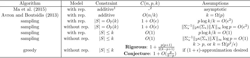
Table 1: Summary of approximation results. Σ∗ =X>diag(π∗)X, where π∗ is the optimal solu-tion of Eq. (4). Sampling based algorithms can be with or without replacement and are randomized, which succeed with at least 0.8 probability.
Algorithm Model Constraint C(n, p, k) Assumptions
Ma et al. (2015) with rep. additive1 -2 asymptotic
Avron and Boutsidis (2013) with rep. additive O(n/k) k= Ω(p)
sampling with rep. |S|=OP(k) 1 +O() plogk/k=O(2)
sampling without rep. |S|=OP(k) 1 +O() kΣ
−1
∗ k2κ(Σ∗)kXk∞logp=O(2)
sampling with rep. |S| ≤k O(1) plogk/k=O(1)
sampling without rep. |S| ≤k O(1) kΣ−1
∗ k2κ(Σ∗)kXk∞logp=O(1)
greedy without rep. |S| ≤k Rigorous: 1 +
p(p+1) 2(k−p+1)
Conjecture: 1 +O(k−pp)
k > p, ork= Ω(p2/) if (1 +)-approximation desired
Definition 2 (C(n, p, k)-approximate algorithm) Fix n ≥ k ≥ p and b ∈ {1,2}. We say an algorithm (either deterministic or randomized)A∈ Ab(k)is aC(n, p, k)-approximate algorithm if for any X∈Rn×p with full column rank, A produces a subset S⊆[n]with size k and an estimateβbA in polynomial time such that, with probability at least 0.8,
sup
β0∈Rp
E
h
kβbA−β0k22 XS
i
≤C(n, p, k)· inf
A0∈A
b(k)
sup
β0∈Rp
E
h
kβbA0−β0k22 i
. (3)
Here both expectations are taken over the randomness in the noise variables eε and the inherent randomness in A.
Table 1 gives an overview of approximation ratio C(n, p, k) for algorithms proposed in this paper. We remark that the combinatorial A-optimality solution of Eq. (1) upper bounds the minimax risk (since minimaxity is defined over deterministic algorithms as well), hence the approximation guarantees also hold with respect to the combinatorial A-optimality objective.
2.1 Related work
There has been an increasing amount of work on fast solvers for the general least-square problem minβky −Xβk22. Most of existing work along this direction (Woodruff, 2014; Dhillon et al., 2013; Drineas et al., 2011; Raskutti and Mahoney, 2015) focuses solely on the computational aspects and do not consider statistical constraints such as limited measure-ments ofy. A convex optimization formulation was proposed in Davenport et al. (2015) for a constrained adaptive sensing problem, which is a special case of our setting, but without finite sample guarantees with respect to the combinatorial problem. In Horel et al. (2014) a computationally tractable approximation algorithm was proposed for the D-optimality criterion of the experimental design problem. However, the core idea in Horel et al. (2014) of pipage rounding an SDP solution (Ageev and Sviridenko, 2004) is not applicable in our problem because the objective function we consider in Eq. (4) is not submodular.
constraints and statistical properties were also analyzed within the linear regression model (Zhu et al., 2015). However, none of the above-mentioned (computationally efficient) meth-ods achieve near minimax optimal statistical efficiency in terms of estimating the underlying linear modelβ0, since the methods can be worse than uniform sampling which has a fairly large approximation constant for generalX. One exception is Avron and Boutsidis (2013), which proposed a greedy algorithm that achieves an error bound of estimation ofβ0 that is within a multiplicative factor of the minimax optimal statistical efficiency. The multiplica-tive factor is however large and depends on the size of the full sample poolX, as we remark in Table 1 and also in Sec. 3.4.
Another related area isactive learning (Chaudhuri et al., 2015; Hazan and Karnin, 2015; Sabato and Munos, 2014), which is a stronger setting where feedback from prior measure-ments can be used to guide subsequent data selection. Chaudhuri et al. (2015) analyzes an SDP relaxation in the context of active maximum likelihood estimation. However, the analysis in Chaudhuri et al. (2015) only works for the with replacement model and the two-stage feedback-driven strategy proposed in Chaudhuri et al. (2015) is not available under the experiment selection model defined in Definition 1 where no feedback is assumed.
2.2 Notations
For a matrixA ∈Rn×m, we use kAkp = supx6=0 kAxkp
kxkp to denote the inducedp-norm ofA.
In particular, kAk1 = max1≤j≤mPni=1|Aij| and kAk∞ = max1≤i≤nPmj=1|Aij|. kAkF =
q P
i,jA2ij denotes the Frobenius norm ofA. Let σ1(A)≥σ2(A)≥ · · · ≥ σmin(n,m)(A)≥0 be the singular values of A, sorted in descending order. The condition number κ2(A) is defined asκ(A) =σ1(A)/σmin(n,m)(A). For sequences of random variablesXnandYn, we use Xn
p
→Ynto denoteXnconverges in probability toYn. We sayan.bnif limn→∞|an/bn| ≤1
and an & bn if limn→∞|bn/an| ≤1. For two d-dimensional symmetric matrices A and B,
we write A B ifu>(A−B)u ≤ 0 for all u ∈Rd, and A B if u>(A−B)u ≥0 for all
u∈Rd.
3. Methods and main results
We describe two computationally feasible algorithms for the experiment selection problem, both based on a continuous convex optimization problem. Statistical efficiency bounds are presented for both algorithms, with detailed proofs given in Sec. 7.
3.1 Continuous optimization and minimax lower bounds
We consider the following continuous optimization problem, which is a convex relaxation of the combinatorial A-optimality criterion of Eq. (1):
π∗= argminπ∈Rnf(π;X) = argminπ∈
Rptr
X>diag(π)X−1
, (4)
s.t. π≥0, kπk1≤k,
Note that the kπk∞≤1 constraint is only relevant for the without replacement model and for the with replacement model we drop this constraint in the optimization problem. It is easy to verify that both the objective f(π;X) and the feasible set in Eq. (4) are convex, and hence the global optimal solution π∗ of Eq. (4) can be obtained using computation-ally tractable algorithms. In particular, we describe an SDP formulation and a practical projected gradient descent algorithm in Appendix B and D, both provably converge to the global optimal solution of Eq. (4) with running time scaling polynomially in n, p and k.
We first present two facts, which are proved in Sec. 7.
Fact 3.1 Letπ and π0 be feasible solutions of Eq. (4) such thatπi≤π0i for alli= 1,· · · , n.
Then f(π;X)≥f(π0;X), with equality if and only if π =π0.
Fact 3.2 kπ∗k1 =k.
We remark that the inverse monotonicity of f in π implies second fact, which can potentially be used to understand sparsity ofπ∗ in later sections.
The following theorem shows that the optimal solution of Eq. (4) lower bounds the minimax risk defined in Eq. (2). Its proof is placed in Sec. 7.
Theorem 3 Let f1∗(k;X) and f2∗(k;X) be the optimal objective values of Eq. (4) for with replacement and without replacement, respectively. Then for b∈ {1,2},
inf
A∈Ab(k)
sup
β0∈Rp
E
h
kβbA−β0k22 i
≥σ2·fb∗(k;X). (5)
Despite the fact that Eq. (4) is computationally tractable, its solution π∗ isnot a valid experiment selection algorithm under a measurement budget of k because there can be much more thankcomponents inπ∗ that are not zero. In the following sections, we discuss strategies for choosing a subsetSbof rows with|Sb|=OP(k) (i.e., soft constraint) or|Sb| ≤k (i.e., hard constraint), using the solutionπ∗ to the above.
3.2 Sampling based experiment selection: soft size constraint
We first consider a weaker setting wheresoft constraint is imposed on the size of the selected subsetSb; in particular, it is allowed that |Sb|=O(k) with high probability, meaning that a constant fraction of over-selection is allowed. The more restrictive setting of hard constraint is treated in the next section.
A natural idea of obtaining a valid subset S of size k is by sampling from a weighted row distribution specified by π∗. Let Σ∗ =X>diag(π∗)X and define distributionsp(1)j and
p(2)j forj= 1,· · ·, n as
P(1): p(1)j =πj∗x>j Σ−∗1xj/p, with replacement; P(2): p(2)j =πj∗/k, without replacement.
Note that both{p(1)j }n
j=1and{p (2)
j }nj=1sum to one because Pn
j=1π ∗
j =kand
Pn j=1π
∗
jx
>
jΣ
−1 ∗ xj =
tr((Pn
j=1π ∗
jxjx
>
j)Σ
−1
input :X ∈Rn×p, optimal solution π∗, target subset sizek.
output:Sb⊆[n], a selected subset of size at mostOP(k). Initialization: t= 0,S0=∅.
With replacement: for t= 1,· · · , k do: - sampleit∼P(1) and set wt=dπi∗t/(kp
(1)
it )e;
- update: St+1=St∪ {wt repetitions ofxit}.
Without replacement: for i= 1,· · ·, n do: - samplewi ∼Bernoulli(kp(2)j );
- update: Si+1 =Si∪ {wi repetitions ofxi}.
Finally, output Sb=Sk for with replacement andSb=Sn for without replacement. Figure 1:Sampling based experiment selection (expected size constraint).
Under the without replacement setting the distribution P(2) is straightforward: p(2)j is proportional to the optimal continuous weights π∗j; under the with replacement setting, the sampling distribution takes into account leverage scores (effective resistance) of each data point in the conditioned covariance as well. Later analysis (Theorem 5) shows that it helps with the finite-sample condition on k. Figure 1 gives details of the sampling based algorithms for both with and without replacement settings.
The following proposition bounds the size of Sbin high probability:
Proposition 4 For any δ ∈ (0,1/2) with probability at least 1−δ it holds that |Sb| ≤ 2(1 + 1/δ)k. That is, |Sb| ≤OP(k).
Proof Apply Markov’s inequality and note that an additional ksamples need to be added due to the ceiling operator in with replacement sampling.
The sampling procedure is easy to understand in an asymptotic sense: it is easy to verify that EXi>tXit = X
>diag(π∗/k)X and
E[wit] = 1, for both with and without replacement
settings. Note that kp(2)it k∞ ≤ 1/k by feasibility constraints and hence Bernoulli(kp(2)it ) is a valid distribution for all it ∈ [n]. For the with replacement setting, by weak law of
large numbers, X>
b SXSb
p
→ X>diag(π∗)X as k → ∞ and hence tr[(XS>XS)−1] p
→ f(π∗;X) by continuous mapping theorem. A more refined analysis is presented in Theorem 5 to provide explicit conditions under which the asymptotic approximations are valid and on the statistical efficiency ofSbas well as analysis under the more restrictive without replacement regime.
Theorem 5 Fix > 0 as an arbitrarily small accuracy parameter. Suppose the following conditions hold:
With replacement: plogk/k=O(2);
Here Σ∗ = X>diag(π∗)X and κ(Σ∗) denotes the conditional number of Σ∗. Then with probability at least 0.9 the subset OLS estimator βb= (X>
b SXSb)
−1X>
b
SySb satisfies E
h
kβb−β0k22 XSb
i
=σ2trh(X>
b SXSb)
−1i≤(1 +O())·σ2f∗
b(X;k), b∈ {1,2}.
We adapt the proof technique of Spielman and Srivastava in their seminal work on spectral sparsification of graphs (Spielman and Srivastava, 2011). More specifically, we prove the following stronger “two-sided” result which shows thatX>
b
SXSbis aspectral approximation
of Σ∗ with high probability, under suitable conditions.
Lemma 6 Under the same conditions in Theorem 5, it holds that with probability at least 0.9 that
(1−)z>Σ∗z≤z>Σb
b
Sz≤(1 +)z
>Σ
∗z, ∀z∈Rp,
where Σ∗ =X>diag(π∗)X and ΣSb=X>
b SXSb.
Lemma 6 implies that with high probabilityσj(Σb
b
S)≥(1−)σj(Σ∗) for allj = 1,· · · , p.
Recall that tr[(XS>XS)−1] = Ppj=1σj(Σb
b S)
−1 and f(π∗;X) = Pp
j=1σj(Σ∗). Subsequently, for∈(0,1−c] for some constant c >0, tr[(X>
b SXSb)
−1]≤(1 +O())f(π∗;X). Theorem 5 is thus proved.
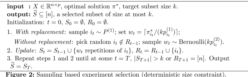
3.3 Sampling based experiment selection: hard size constraint
In some applications it is mandatory to respect a hard subset size constraint; that is, a randomized algorithm is expected to output Sb that satisfies |Sb| ≤ k almost surely, and no over-sampling is allowed. To handle such hard constraints, we revise the algorithm in Figure 1 as follows:
input :X ∈Rn×p, optimal solution π∗, target subset sizek.
output:Sb⊆[n], a selected subset of size at mostk. Initialization: t= 0,S0=∅,R0 =∅.
1. With replacement: sample it∼P(1); set wt=dπi∗t/(kp
(1)
it )e;
Without replacement: pick random it∈/ Rt−1; samplewt∼Bernoulli(kp(2)it ).
2. Update: St=St−1∪ {wtrepetitions of it},Rt=Rt−1∪ {it}.
3. Repeat steps 1 and 2 until at somet=T,|ST+1|> kor RT+1 = [n]. Output b
S=ST.
Figure 2:Sampling based experiment selection (deterministic size constraint).
We have the following theorem, which mimics Theorem 5 but with weaker approximation bounds:
Theorem 7 Suppose the following conditions hold: with replacement: plogk/k=O(1);
Then with probability at least 0.8 the subset estimator βb= (X>
b SXSb)
−1X>
SyS satisfies
E
h
kβb−β0k22 XSb
i
=σ2tr h
(X>
b SXSb)
−1i≤O(1)·σ2f∗
b(X;k), b∈ {1,2}.
The following lemma is key to the proof of Theorem 7. Unlike Lemma 6, in Lemma 8 we only prove one side of the spectral approximation relation, which suffices for our purposes. To handle without replacement, we cite matrix Bernstein for combinatorial matrix sums in (Mackey et al., 2014).
Lemma 8 Define Σb
b
S=X
>
b
SXSb. Suppose the following conditions hold:
With replacement: plogT /T =O(1);
Without replacement: kΣ−∗1k2κ(Σ∗)kXk2∞logp=O(T /n). Then with probability at least 0.9 the following holds:
z>Σb
b
Sz≥KTz
>Σ
∗z, ∀z∈Rp, (6)
where KT = Ω(T /k) for with replacement andKT = Ω(T /n) for without replacement.
Finally, we need to relate conditions on T in Lemma 8 to interpretable conditions on subset budget k:
Lemma 9 Let δ >0be an arbitrarily small fixed failure probability. The with probability at least 1−δ we have that T ≥δk for with replacement and T ≥δn for without replacement. Proof For with replacement we haveE[PTt=1wt] =T and for without replacement we have E[PTt=1wt] =T k/n. Applying Markov’s inequality on Pr[PTt=1wt> k] for T =δk and/or T =δnwe complete the proof of Lemma 9.
Combining Lemmas 8 and 9 with δ = 0.1 and note that T ≤ k almost surely (because
wt≥1), we prove Theorem 7.
3.4 Greedy experiment selection
input :X ∈Rn×p, Initial subset S
0⊆[n], target size k≤ |S0|. output:Sb⊆[n], a selected subset of sizek.
Initialization: t= 0.
1. Find j∗ ∈St such that tr[(XS>t\{j∗}XSt\{j∗})−1] is minimized.
2. Remove j∗ from St: St+1=St\{j∗}.
3. Repeat steps 1 and 2 until|St|=k. OutputSb=St. Figure 3: Greedy experiment selection.
Lemma 10 SupposeSb⊆[n]of sizekis obtained by running algorithm in Figure 3 with an initial subsetS0 ⊆[n],|S0| ≥k. BothSbandS0 are standard sets (i.e., without replacement). Then
tr h
(X>
b SXSb)
−1i≤ |S0| −p+ 1
k−p+ 1 tr h
(XS>0XS0)
−1i.
In Avron and Boutsidis (2013) the greedy removal procedure in Figure 3 is applied to the entire design set S0 = [n], which gives approximation guarantee tr[(X>
b SXSb)
−1] ≤
n−p+1
k−p+1tr[(X
>X)−1]. This results in an approximation ratio ofC(n, p, k) = n−p+1
k−p+1 as defined in Eq. (2), by applying the trivial bound tr[(X>X)−1] ≤ f∗
2(k;X), which is tight for a design that has exactlyk non-zero rows.
To further improve the approximation ratio, we consider applying the greedy removal procedure with S0 equal to the support of π∗; that is, S0 = {j ∈ [n] : πj∗ > 0}. Because
kπ∗k∞≤1 under the without replacement setting, we have the following corollary:
Corollary 11 Let S0 be the support ofπ∗ and suppose kπ∗k∞≤1. Then tr[(X>
b SXSb)
−1]≤ kπ∗k0−p+ 1
k−p+ 1 f(π ∗
;X) = kπ ∗k
0−p+ 1
k−p+ 1 f ∗ 2(k;X).
It is thus important to upper bound the support size kπ∗k0. With the trivial bound of
kπ∗k0 ≤n we recover the nk−−pp+1+1 approximation ratio by applying Figure 3 to S0 = [n]. In order to boundkπ∗k0 away from n, we consider the following assumption imposed onX: Assumption 3.1 Define mapping φ:Rp → R
p(p+1)
2 as φ(x) = (ξijx(i)x(j))1≤i≤j≤p, where
x(i) denotes the ith coordinate of a p-dimensional vector x andξij = 1 if i=j and ξij = 2
otherwise. Denote φe(x) = (φ(x),1) ∈ R
p(p+1)
2 +1 as the affine version of φ(x). For any
p(p+1)
2 + 1 distinct rows ofX, their mappings underφeare linear independent.
Assumption 3.1 is essentially a general-position assumption, which assumes that no
p(p+1)
2 + 1 design points in X lie on a degenerate affine subspace after a specific quadratic mapping. Like other similar assumptions in the literature (Tibshirani, 2013), Assumption 3.1 is very mild and almost always satisfied in practice, for example, if each row of X is independently sampled from absolutely continuous distributions.
We are now ready to state the main lemma bounding the support size of π∗.
Lemma 12 kπ∗k0 ≤k+p(p2+1) if Assumption 3.1 holds.
Combining results from both Lemma 12 and Corollary 11 we arrive at the following theorem, which upper bounds the approximation ratio of the greedy removal procedure in Figure 3 initialized by the support of π∗.
Theorem 13 Let π∗ be the optimal solution of the without replacement version of Eq. (4) and Sb be the output of the greedy removal procedure in Figure 3 initialized with S0 = {i ∈ [n] : πi∗ > 0}. If k > p and Assumption 3.1 holds then the subset OLS estimator
b
β = (X>
b SXSb)
−1X>
b
SySb satisfies
E
h
kβb−β0k X
b S
i
=σ2trh(X>
b SXSb)
−1i≤
1 + p(p+ 1) 2(k−p+ 1)
f2∗(k;X).
Under a slightly stronger condition that k > 2p, the approximation ratio C(n, k, p) = 1 + 2(pk(−p+1)p+1) can be simplified to C(n, k, p) = 1 +O(p2/k). In addition, C(n, k, p) = 1 +o(1) if p2/k → 0, meaning that near-optimal experiment selection is achievable with computationally tractable methods ifO(p2) design points are allowed in the selected subset. 3.5 Interpretable subsampling example: anisotropic Gaussian design
Even though we consider a fixed pool of design points so far, here we use an anisotropic Gaussian design example to demonstrate that a non-uniform sampling can outperform uni-form sampling even under random designs, and to interpret the conditions required in previous analysis. Let x1,· · · , xn be i.i.d. distributed according to an isotropic Gaussian
distributionNp(0,Σ0).
We first show that non-uniform weights πi 6=k/n could improve the objectivef(π;X).
Letπunif be the uniformly weighted solution ofπunif
i =k/n, corresponding to selecting each
row ofX uniformly at random. We then have
f(πunif;X) = 1
ktr
"
1
nX
>X
−1#
p
→ 1
ktr(Σ
−1 0 ).
On the other hand, let B2 =γtr(Σ0) for some universal constant γ >1 and B={x∈Rp:
kxk2
2 ≤ B2}, X = {x1,· · ·, xn}. By Markov inequality, |X∩B| & 1γn−γ. Define weighted
solution πw as πwi ∝1/p(xi|B)·I[xi∈B] normalized such thatkπiwk1 =k. 1 Then
f(πw;X) = 1
k
tr
1
n
P
xi∈X∩B
xix>i
p(xi|B) −1 1
n
P
xi∈X∩B1/p(xi|B)
p
→ 1
k n |X∩B|
tr h
R Bxx
>dx−1i R
B1dx
. p
2 (1−γ)tr(Σ0).
Here in the last inequality we apply Lemma 17. Because tr(Σ
−1 0 )
p =
1
p
Pp
i=1σi(Σ10) ≥
1
p
Pp
i=1σi(Σ0) −1
= tr(Σp
0) by Jensen’s inequality, we conclude that in generalf(π
w;X)<
f(πunif;X), and the gap is larger for ill-conditioned covariance Σ
0. This example shows that uneven weights in π helps reducing the trace of inverse of the weighted covariance
X>diag(π)X.
Under this model, we also simplify the conditions for the without replacement model in theorem 5 and 7. Becausex1,· · ·, xn
i.i.d.
∼ Np(0,Σ0), it holds thatkXk2∞≤OP(kΣ0k 2
2plogn). In addition, by simple algebra kΣ−∗1k2 ≤ p−1κ(Σ∗)tr(Σ∗−1) ≤ p−1κ(Σ∗)f1∗(k;X). Using a very conservative upper bound of f1∗(k;X) by sampling rows in X uniformly at random and apply weak law of large numbers and the continuous mapping theorem, we have that
f1∗(k;X). k1tr(Σ
−1
0 ). In addition, tr(Σ −1
0 )kΣ0k2 ≤pkΣ0−1k2kΣ0k2 =pκ(Σ0). Subsequently, the conditionkΣ−∗1k2κ(Σ∗)kXk2∞logp=O(2) is implied by
pκ(Σ∗)2κ(Σ0) logplogn
k =O(
2). (7)
Essentially, the condition is reduced to k & κ(Σ0)κ(Σ∗)·plognlogp. The linear depen-dency on p is necessary, as we consider the low-dimensional linear regression problem and k < p would imply an infinite mean-square error in estimation of β0. We also re-mark that the condition is scale-invariant, as X0 = ξX and X share the same quantity
kΣ−∗1k2κ(Σ∗)kXk2∞logk. 3.6 Extensions
We discuss possible extension of our results beyond estimation ofβ0 in the linear regression model.
3.6.1 Generalized linear models
In a generalized linear model µ(x) = E[Y|x] satisfies g(µ(x)) = η = x>β0 for some known link function g : R → R. Under regularity conditions (Van der Vaart, 2000), the
maximum-likelihood estimator βbn ∈argmaxβ{ Pn
i=1logp(yi|xi;β)}satisfies Ekβbn−β0k22 = (1 +o(1))tr(I(X, β0)−1), whereI(X, β0) is the Fisher’s information matrix:
I(X, β0) =−
n
X
i=1
E∂
2logp(y
i|xi;β0) ∂β∂β> =−
n
X
i=1
E∂
2logp(y
i;ηi) ∂η2
i
xix>i . (8)
Here both expectations are taken overyconditioned onXand the last equality is due to the sufficiency of ηi =x>i β0. The experiment selection problem is then formulated to select a subsetS ⊆[n] of size k, either with or without duplicates, that minimizes tr(I(XS, β0)−1).
It is clear from Eq. (8) that the optimal subsetS∗ depends on the unknown parameter
β0, which itself is to be estimated. This issue is known as thedesign dependenceproblem for generalized linear models (Khuri et al., 2006). One approach is to consider locally optimal designs (Khuri et al., 2006; Chernoff, 1953), where a consistent estimate ˇβ of β0 is first obtained on an initial design subset 2 and then ˇηi = x>i βˇ is supplied to compute a more 2. Notice that a consistent estimate can be obtained using much fewer points than an estimate with finite
refined design subset to get the final estimateβb. With the initial estimate ˇβ available, one may apply transform xi 7→exi defined as
e
xi =
s −E∂
2logp(y
i; ˇηi) ∂η2 xi. Note that under regularity conditions−E∂
2logp(y
i;ˇηi)
∂η2
i
=E
∂log(y
i;ˇxi)
∂ηi
2
is non-negative and hence the square-root is well-defined. All results in Theorems 5, 7 and 13 are valid with
X = [x1,· · · , xn]> replaced by Xe = [xe1,· · · ,exn]> for generalized linear models. Below we consider two generalized linear model examples and derive explicit forms of Xe.
Example 1: Logistic regression In a logistic regression model responsesyi ∈ {0,1}are
binary and the likelihood model is
p(yi;ηi) =ψ(ηi)yi(1−ψ(ηi))1−yi, where ψ(ηi) = eηi
1 +eηi.
Simple algebra yields
e
xi =
s
eηˇi
(1 +eηˇi)2xi,
where ˇηi =x>i βˇ.
Example 2: Poisson count model In a Poisson count model the response variable
yi takes values of non-negative integers and follows a Poisson distribution with parameter λ=eηi =ex>i β0. The likelihood model is formally defined as
p(yi=r;ηi) =
eηire−eηi
r! , r= 0,1,2,· · · . Simple algebra yields
e
xi =
√ eηˇixi,
where ˇηi =x>i βˇ.
3.6.2 Delta’s method
Suppose g(β0) is the quantity of interest, where β0 ∈ Rp is the parameter in a linear
regression model and g : Rp → Rm is some known function. Let βbn = (X>X)−1X>y be the OLS estimate of β0. If ∇g is continuously differentiable and βbn is consistent, then by the classical delta’s method (Van der Vaart, 2000) Ekg(βbn)−g(β0)k22 = (1 +
o(1))σ2tr(∇g(β0)(X>X)−1∇g(β0)>) = (1+o(1))σ2tr(G0(X>X)−1), whereG0 =∇g(β0)>∇g(β0). If G0 depends on the unknown parameter β0 then the design dependence problem again exists, and a locally optimal solution can be obtained by replacing G0 in the objective function with ˇG=∇g( ˇβ)>∇g( ˇβ) for some initial estimate ˇβ of β0.
If ˇGis invertible, then there exists invertiblep×pmatrix ˇP such that ˇG= ˇPPˇ>because ˇ
Gis positive definite. Applying the linear transform
xi 7→exi = ˇP
−1x
i
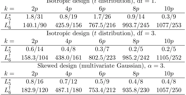
Table 2: Running time (seconds) / no. of iterations forL∗5 andL†6. Isotropic design (tdistribution), df = 1.
k= 2p 4p 6p 8p 10p
L∗5 1.8/31 0.8/19 1.7/26 0.9/14 0.3/9
L†6 140.1/90 425.9/156 767.5/216 993.7/245 1077/253 Isotropic design (tdistribution), df = 3.
k= 2p 4p 6p 8p 10p
L∗5 0.6/14 0.4/8 0.3/7 0.2/5 0.2/5
L†6 158.3/104 438.0/161 802.5/223 985.2/242 1105/252 Skewed design (multivariate Gaussian),α = 3.
k= 2p 4p 6p 8p 10p
L∗5 0.8/16 0.7/12 0.5/9 0.4/8 0.4/8
L†6 182.9/120 487.1/180 753.4/212 935.8/230 1057/250
Example: prediction error. In some application scenarios the prediction error kZβb−
Zβ0k22 rather than the estimation errorkβb−β0k22 is of interesting, either because the linear model is used mostly for prediction or component of the underlying model β0 lack physical interpretations. Another interesting application is the transfer learning (Pan and Yang, 2010), in which the training and testing data have different designs (e.g., Z instead of X) but share the same conditional distribution of labels, parameterized by the linear modelβ0. SupposeZ ∈Rm×p is a known full-rank data matrix upon which predictions are seeked,
and define ΣbZ = m1Z>Z 0 to be the sample covariance of Z. Our algorithmic frame-work as well as its corresponding analysis remain valid for such prediction problems with transform xi 7→ Σb
−1/2
Z xi. In particular, the guarantees for the greedy algorithm and the
with replacement sampling algorithm remain unchanged, and the guarantee for the without replacement sampling algorithm is valid as well, except that the kΣ−∗1k2 and κ(Σ∗) terms have to be replaced by the (relaxed) optimal sample covariance after the linear transform
xi 7→Σb
−1/2
Z xi.
4. Numerical results on synthetic data
We report selection performance (measured in terms ofF(S;X) := tr[(XS>XS)−1] which is
the mean squared error of the ordinary least squares estimator based on (XS, yS) in
esti-mating the regression coefficients) on synthetic data. Only the without replacement setting is considered, and results for the with replacement setting are similar. In all simulations, the experimental pool (number of given design points)nis set to 1000, number of variables
Figure 1: The ratio of MSE kβb−β0k22 compared against the MSE of the OLS estimator on the
full data pool kβbols −β0k22, βbols = (X>X)−1X>y, and objective values F(Sb;X) = tr[(X>
b SXSb)
−1] on synthetic data sets. Note that the L
5 (greedy) curve is under the
4.1 Data generation
The design pool X is generated so that each row of X is sampled from some underlying distribution. We consider two distributional settings for generating X. Similar settings were considered in (Ma et al., 2015) for subsampling purposes.
1. Distributions with skewed covariance: each row of X is sampled i.i.d. from a mul-tivariate Gaussian distribution Np(0,Σ0) with Σ0 = UΛU>, where U is a random
orthogonal matrix and Λ = diag(λ1,· · · , λp) controls the skewness or conditioning of X. A power-law decay of λ, λj = j−α, is imposed, with small α corresponding to
“flat” distribution and large α corresponding to “skewed” distribution. Rows 1-2 in Figure 1 correspond to this setting.
2. Distributions with heavy tails: We use t distribution as the underlying distribution for generating each entry inX, with degrees of freedom ranging from 2 to 4. These distributions are heavy tailed and high-order moments of X typically do not exist. They test the robustness of experiment selection methods. Rows 3-4 in Figure 1 correspond to this setting.
4.2 Methods
The methods that we compare are listed below:
- L1 (uniform sampling): each row of X is sampled uniformly at random, without replacement.
- L2 (leverage score sampling): each row of X, xi, is sampled without replacement,
with probability proportional to its leverage score x>i (X>X)−1x
i. This strategy is
considered in Ma et al. (2015) for subsampling in linear regression models.
- L3 (predictive length sampling): each row ofX,xi, is sampled without replacement,
with probability proportional to its `2 norm kxik2. This strategy is derived in Zhu
et al. (2015).
- L∗4 (sampling based selection withπ∗): the sampling based method that is described in Sec. 3.3, based on π∗, the optimal solution of Eq. (4). We consider the hard size constraint algorithm only.
- L∗5 (greedy based selection with π∗): the greedy based method that is described in Sec. 3.4.
20 22 24 26 28 30 number of experiments (k) 1
1.5 2 2.5 3
MSE of y
Linear regression L1 (unif) L2 (lev) L3 (PL) L4 (sampling) L5 (greedy) L6 (fedorov)
20 22 24 26 28 30
number of experiments (k) 0
0.2 0.4 0.6 0.8 1
MSE of
β0
(
×
10
2)
Linear regression L1 (unif) L2 (lev) L3 (PL) L4 (sampling) L5 (greedy) L6 (fedorov)
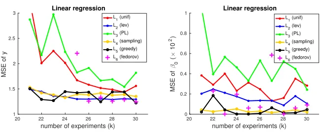
Figure 2: Results on real material synthesis data (n= 133, p= 9,20< k ≤30). Left: prediction error ky −Xβbk22, normalized by dividing by the prediction error ky−Xβbolsk22 of the OLS estimator on the full data set; right: estimation error kβb−βbolsk22. All random-ized algorithms (L1, L2, L3, L∗4, L
†
6) are run for 50 times and the median performance is
reported.
4.3 Performance
The ratio of the mean square error kβb−β0k22 compared to the OLS estimator on the full data setkβbols−β0k22,βbols= (X>X)−1X>y, and objective valuesF(Sb;X) = tr((X>
b SXSb)
−1) are reported in Figure 1.
Table 2 reports the running time and number of iterations ofL∗5 (greedy based selection) andL†6 (Fedorov’s exchange algorithm). In general, the greedy method is 100 to 1000 times faster than the exchange algorithm, and also converges in much fewer iterations.
For both synthetic settings, our proposed methods (L∗4 and L∗5) significantly outper-form existing approaches (L1, L2, L3), and their performance is on par with the Fedorov’s exchange algorithm, which is much more computationally expensive (cf. Table 2).
5. Numerical results on real data
5.1 The material synthesis dataset
We apply our proposed methods to an experimental design problem of low-temperature microwave-assisted crystallization of ceramic thin films (Reeja-Jayan et al., 2012; Nakamura et al., 2017). The microwave-assisted experiments were controlled by four experimental parameters: temperatureT (120◦C to 170◦C), hold timeH (0 to 60 minutes), ramp power
P (0W to 60W) and tri-ethyl-gallium (TEG) volume ratioR(from 0 to 0.93). A generalized quadratic regression model was employed in (Nakamura et al., 2017) to estimate the coverage percentage of the crystallization CP:
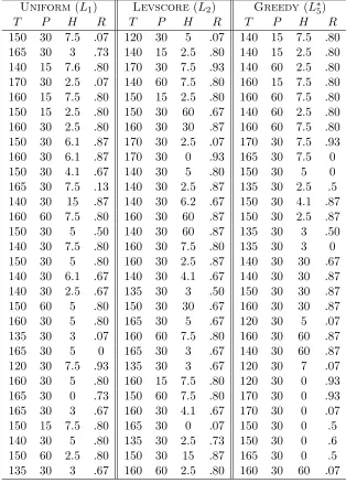
Table 3: Selected subsets of uniform sampling (Uniform), leverage score sampling (Levscore) and greedy method (Greedy) on the material synthesis dataset.
Uniform (L1) Levscore(L2) Greedy (L∗5)
T P H R T P H R T P H R
Table 4: Comparison of the “true” modelβ0= [0.49; 0.30; 0.19; 3.78] and the subsampled estimators
b
β for different components ofβ. kis the number of subsamples. Random algorithms (L1
throughL∗4) are repeated for 100 times and the median difference is reported.
∆β1 ∆β2 ∆β3 ∆β4 k∆βk2 ∆β1 ∆β2 ∆β3 ∆β4 k∆βk2
k= 20 k= 30
L1 .043 .071 .074 .274 .295 L1 .038 .064 .070 .171 .199
L2 .017 .026 .018 .260 .263 L2 .011 .024 .014 .199 .201
L3 .017 .043 .026 .243 .249 L3 .015 .031 .018 .236 .239
L∗4 .014 .039 .114 .215 .247 L∗4 .014 .023 .030 .044 .060
L∗5 .010 .024 .032 .209 .213 L∗5 .022 .000 .050 .088 .104
L†6 .010 .024 .032 .209 .213 L†6 .022 .000 .050 .088 .104
k= 50 k= 75
L1 .025 .035 .037 .130 .142 L1 .016 .032 .024 .133 .139
L2 .009 .027 .012 .130 .134 L2 .006 .034 .010 .126 .131
L3 .011 .035 .013 .166 .170 L3 .009 .029 .009 .124 .128
L∗4 .022 .009 .036 .097 .106 L∗4 .012 .001 .015 .036 .041
L∗5 .025 .003 .040 .009 .048 L∗5 .005 .013 .009 .016 .023
L†6 .025 .003 .040 .009 .048 L†6 .005 .012 .010 .011 .020
from 21 to 30, and report in Figure 2 the mean-square error (MSE) of both the prediction error ky−Xβbk22, normalized by dividing by the prediction error ky−Xβbolsk22 of the OLS estimator on the full data set, on the full 133 experiments and the estimation error kβb−
b
βolsk2
2. Figure 2 shows that our proposed methods consistently achieve the best performance and are more stable compared to uniform sampling and Fedorov’s exchange methods, even though the linear model assumption may not hold.
We also report the actual subset (k = 30) design points selected by uniform sampling (L1), leverage score sampling (L3) and our greedy method (L∗5) in Table 3. Table 3 shows that the greedy algorithm (L∗5) picked very diverse experimental settings, including several settings of very lower temperature (120◦C) and very short hold time (0). In contrast, the experiments picked by both uniform sampling (L1) and leverage score sampling (L3) are less diverse.
5.2 The CPU performance dataset
man-ufacturing process. The learned model can also be used to predict the relative performance of a new CPU model based on its model parameters, without running extensive benchmark tests.
Using domain knowledge, Ein-Dor and Feldmesser (1987) narrow down to three param-eters of interest: average memory size (X1),cache size (X2) andchannel capacity (X3), all being explicitly computable functions from CPU model parameters. An offset parameter is also involved in the linear regression model, making the number of variables p = 4. A total ofn= 209 CPU models are considered, with all of the model parameters and relative performance collected and no missing data. Stepwise linear regression was applied to obtain the following linear model:
0.49X1+ 0.30X2+ 0.19X3+ 3.78. (10) To use this data set as a benchmark for evaluating the experiment selection methods, we synthesize labels Y using model Eq. (10) with standard Gaussian noise and measure the difference between fit βband the true model β0 = [0.49; 0.30; 0.19; 3.78]. Table 4 shows that under various measurement budget (k) constraints, the proposed methods L∗4 and L∗5
consistently achieve small estimation error, and is comparable to the Fedorov’s exchange algorithm (L†6). As the data set is small (209×4), all algorithms are computationally efficient.
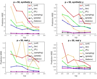
5.3 The Minnesota Wind Dataset
The Minnesota wind dataset collects wind speed information across n= 2642 locations in Minnesota, USA for a period of 24 months (for the purpose of this experiment, we only use wind speed data for one month). The 2642 locations are connected with 3304 bi-directional roads, which form an n×n sparse unweighted undirected graph G. Let L= diag(d)−G
be the n×nLaplacian of G, where dis a vector of node degrees and let V ∈ Rn×p be an
orthonormal eigenbasis corresponding to the smallestpeigenvalues ofL. As the wind speed signaly∈Rnis relatively smooth, it can be well-approximated asy=V θ+ε, whereθ∈Rp
corresponds to the coefficients of the graph Laplacian basis. The speed signaly has a fast decay on the Laplacian basisV; in particular, OLS on the firstp= 50 basis accounts for over 99% of the variation iny. (That is,kVθbols−yk22≤0.01kyk22, whereθbols= (V>V)−1V>y.)
In our experiments we compare the 6 algorithms (L1 through L6) when a very small portion of the full samples is selected. The ratio of the mean-square prediction error n1kVθb−
yk2
2compared to the MLE of the full-sample OLS estimator n1kVθbols−yk22is reported. Apart from the real speed data, we also report results under a “semi-synthetic” setting similar to Sec. 5.2, where the full OLS estimate θbols is first computed and then y is synthesized as
y=Vbθols+εwhere εare i.i.d. standard Normal random variables.
1.9 2 2.1 2.2 2.3 2.4 2.5 2.6 k/p 2 3 4 5 6 7 8 Prediction MSE
p = 50, synthetic y L
1 (unif)
L
2 (lev)
L3 (PL)
L4 (sampling) L
5 (greedy)
L
6 (fedorov)
2.4 2.5 2.6 2.7 2.8 2.9 3 3.1
k/p 1.4 1.6 1.8 2 2.2 2.4 2.6 2.8 3 Prediction MSE
p = 50, synthetic y L
1 (unif)
L
2 (lev)
L3 (PL)
L4 (sampling) L
5 (greedy)
L
6 (fedorov)
1.9 2 2.1 2.2 2.3 2.4 2.5 2.6
k/p 0.4 0.6 0.8 1 1.2 1.4 Prediction MSE
p = 50, real y
L1 (unif) L2 (lev) L
3 (PL)
L
4 (sampling)
L5 (greedy) L6 (fedorov)
2.4 2.5 2.6 2.7 2.8 2.9 3 3.1
k/p 0.2 0.25 0.3 0.35 0.4 0.45 0.5 0.55 0.6 Prediction MSE
p = 50, real y L
1 (unif) L
2 (lev) L3 (PL)
L4 (sampling) L5 (greedy)
L6 (fedorov)
Figure 3: Plots of the ratio of mean square prediction error n1kVθb−yk22 compared against the MSE of the full-sample OLS estimator 1
nkVθb
ols−yk2
2 on the Minnesota wind dataset.
In the top panel response variablesy are synthesized asy =Vθbols+ε, wherebθols is the full-sample OLS estimator and ε are i.i.d. standard Normal random variables. In the bottom panel the real wind speed responsey is used. For randomized algorithms (L1 to
L4) the experiments are repeated for 50 times and the median MSE ratio is reported.
sufficiently large subset size (e.g., k = 3p), the performance gap between all methods is smaller on real signal compared to the synthetic signals. We conjecture that this is because the linear modely=V θ+εonly approximately holds in real data.
6. Discussion
We discuss potential improvements in the analysis presented in this paper.
6.1 Sampling based method
To fully understand the finite-sample behavior of the sampling method introduced in Secs. 3.2 and 3.3, it is instructive to relate it to the graph spectral sparsification problem (Spielman and Srivastava, 2011) in theoretical computer science: Given a directed weighted graph
z∈R|V|:
(1−) X (u,v)∈E
wuv(zu−zv)2 ≤
X
(u,v)∈Ee
e
wuv(zu−zv)2 ≤(1 +)
X
u,v∈E
wuv(zu−zv)2.
Define BG ∈ R|E|×|V| to be the signed edge-vertex incidence matrix, where each row of
BG corresponds to an edge in E, each column of BG corresponds to a vertex in G, and
[BG]ij = 1 if vertex j is the head of edge i, [BG]ij = −1 if vertex j is the tail of edge i,
and [BG]ij = 0 otherwise. The spectral sparsification requirement can then be equivalently
written as
(1−)z>(B>GW BG)z≤z>(BG>efW B
e
G)z≤(1 +)z
>(B>
GW BG)z.
The similarity of graph sparsification and the experimental selection problem is clear:
BG ∈ Rn×p would be the known pool of design points and W = diag(π∗) is a diagonal
matrix with the optimal weightsπ∗ obtained by solving Eq. (4). The objective is to seek a small subset of rows inBG(i.e., the sparsified edge setEe) which is a spectral approximation of the original BG>diag(π∗)BG. Approximation of the A-optimality criterion or any other
eigen-related quantity immediately follows. One difference is that in linear regression each row of BG is no longer a {±1,0} vector. Also, the subsampled weight matrix fW needs to correspond to an unweighted graph for linear regression, i.e. diagonal entries ofWf must be in {0,1}. However, we consider this to be a minor difference as it does not interfere with the spectral properties ofBG.
The spectral sparsification problem where fW can be arbitrarily designed (i.e. not re-stricted to have{0,1}diagonal entries) is completely solved (Spielman and Srivastava, 2011; Batson et al., 2012), where the size of the selected edge subset is allowed to be linear to the number of vertices, or in the terminology of our problem, k p. Unfortunately, both methods require the power of arbitrary designing the weights inWf, which is generally not available in experiment selection problems (i.e., cannot set noise variance or signal strength arbitrarily for individual design points). Recently, it was proved that when the original graph is unweighted (W =I), it is also possible to find unweighted linear-sized edge spar-sifiers (fW ∝ I) (Marcus et al., 2015a,b; Anderson et al., 2014). This remarkable result leads to the solution of the long-standing Kardison-Singer problem. However, the condition that the original weights W are uniform is not satisfied in the linear regression problem, where the optimal solutionπ∗ may be far from uniform. The experiment selection problem somehow falls in between, where an unweighted sparsifier is desired for a weighted graph. This leads us to the following question:
Question 6.1 Given a weighted graph G = (V, E, W), under what conditions are there small edge subset Ee ⊆ E with uniform weights Wf ∝ I such that Ge = (V,E,e fW) is a (one-sided) spectral approximation of G?
0 20 40 60 80 100 p
0 100 200 300 400 500
||
π
*||
0
-k
||π*||
0-k against p
df=3 df=5 df=10
0 20 40 60 80 100
p 0
100 200 300 400 500
||
π
*||
0
-k
||π*||0-k against p
α=1
α=2
α=3
α=5
Figure 4: Empirical verification of the rate ofkπ∗k0. Left: isotropic design (tdistribution); Right:
skewed design (transformed multivariate Gaussian) with spectral decayλj ∝j−α.
6.2 Greedy method
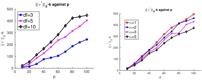
Corollary 11 shows that the approximation quality of the greedy based method depends crucially uponkπ∗k0, the support size of the optimal solutionπ∗. In Lemma 12 we formally established thatkπ∗k0≤k+p(p+ 1)/2 under mild conditions; however, we conjecture the
p(p+ 1)/2 term is loose and could be improved toO(p) in general cases.
In Fig 4 we plotkπ∗k0−kagainst number of variablesp, where pranges from 10 to 100 and k is set to 3p. The other simulation settings are kept unchanged. We observe that in all settingskπ∗k0−kscales linearly withp, suggesting thatkπ∗k0 ≤k+O(p). Furthermore, the slope of the scalings does not seem to depend on the conditioning of X, as shown in the right panel of Fig 4 where the conditioning of X is controlled by the spectral decay rate α. This is in contrast to the analysis of the sampling based method (Theorem 5), in which the finite sample bound depends crucially upon the conditioning ofXfor the without replacement setting.
6.3 High-dimensional settings
This paper focuses solely on the so-called large-sample, low-dimensional regression setting, where the number of variablesp is assumed to be much smaller than both design pool size
n and subsampling size k. It is an interesting open question to extend our results to the high-dimensional setting, wherepis much larger than bothnandk, and an assumption like sparsity of β0 is made to make the problem feasible, meaning that very few components in
β0 are non-zero. In particular, it is desirable to find a sub-sampling algorithm that attains the following minimax estimation rate over high-dimensional sparse models:
inf
A∈Ab(k)
sup kβ0k0≤s
EA,β0
h
kβb−β0k22 i
.
of optimizing such restricted eigenvalues could be even harder and remains largely open. We also mention that Davenport et al. (2015) suggests a two-step approach where half the budget is used to identify the sparse locations from randomly sampled points and the remaining budget is used to generate a better estimate of regression coefficients using the same convex programming formulation proposed in our paper. Their paper provides some experimental support for this idea, however, no theoretical guarantees are established for the (sub)optimality of such a procedure. Analyzing such a two-step approach could be an interesting future direction.
6.4 Approximate linear models
In cases when the linear model y = Xβ0 +ε only approximately holds, we describe here a method that takes into consideration both bias and variance of OLS estimates on sub-sampled data in order to find good sub-samples. Suppose y = f0(X) +ε for some un-known underlying function f0 that might not be linear, and let β∗ = (X>X)−1X>f0(X) be the optimal linear predictor on the full sample X. Suppose XS = ΨX is the
sub-sampled data, where Ψ ∈ R|S|×n is the subsampling matrix where each row of Ψ is ei = (0,· · · ,0,1,0,· · · ,0) ∈ Rn, with i ∈ [n] being the subsampled rows in X. Let
b
β = (XS>XS)−1XS>yS be the OLS on the subsampled data. The error of βb can then be decomposed and upper bounded as
Ekβb−β∗k22=f0(X)> h
(X>Ψ>ΨX)−1X>Ψ>Ψ−(X>X)−1X>if0(X) +σ2tr h
(X>Ψ>ΨX)−1i (11)
≤ (X
>
Ψ>ΨX)−1X>Ψ>Ψ−(X>X)−1X>
op· kf0(X)k 2
2+σ2tr h
(X>Ψ>ΨX)−1 i
.
(12)
In the high noise setting, the first term can be ignored and the solution is close to the one considered in this paper. In the low-noise setting, the second term can be ignored and a relaxation similar to Eq. (4) can be derived; however a linear approximation may be undesirable in this case. In general, when kf0(X)k2
2≈λis known or can be estimated, the following continuous optimization problem serves as an approximate objective of subsampled linear regression with approximate linear models:
min
π∈Rn
λ
n
X
i=1
πixix>i
!−1
X>diag(π)−(X>X)−1X>
op
+σ2tr
n
X
i=1
πixix>i
!−1
s.t. n
X
i=1
πi≤k, 0≤πi≤1.
7. Proofs
7.1 Proof of facts in Sec. 3.1
Proof [Proof of Fact 3.1] Let A = X>diag(π)X and B = X>diag(π0)X. By definition,
B =A+ ∆ where ∆ =X>diag(π0−π)X is positive semi-definite. Subsequently, σ`(B)≥ σ`(A) for all `= 1,· · ·, p. We then have that
f(π0;X) = tr(B−1) =
p
X
`=1
σ`(B)−1≤ p
X
`=1
σ`(A)−1 = tr(A−1) =f(π;X).
Note also that ifπ0 6=πthen ∆6= 0 and hence there exists at least one`withσ`(B)< σ`(A).
Therefore, the equality holds if and only if π=π0.
Proof [Proof of Fact 3.2] Suppose kπ∗k1 < k. Then there exists some coordinate j ∈
{1,· · ·, n}such thatπ∗j <1. Defineπ0 asπi0 =πi∗ fori6=jandπ0j = min{1, πj∗+k− kπ∗k1}. Thenπ0 is also a feasible solution. On the other hand, By Fact 3.1 we have thatf(π0;X)< f(π∗;X), contradicting the optimality of π∗. Therefore, kπ∗k1 =k.
7.2 Proof of Theorem 3
We only prove Theorem 3 for the with replacement setting (b = 1). The proof for the without replacement setting is almost identical.
Define Ae1(k) as the class ofdeterministic algorithms that proceed as follows:
1. The algorithm deterministically outputs pairs {(wi, xi)}Mi=1, where xi is one of the
rows in X and {wi}ni=1 satisfies wi ≥0, PMi=1wi ≤k. Here M is an arbitrary finite
integer.
2. The algorithm observes{yi}Mi=1withyi=
√
wix>i β+εi. Hereβis a fixed but unknown
regression model andεi i.i.d.
∼ N(0, σ2) is the noise.
3. The algorithm outputsβbas an estimation ofβ, based on the observations {yi}Mi=1. Because all algorithms inAe1(k) are deterministic and the design matrix still has full column rank, the optimal estimator of βb given {(wi, xi)}Mi=1 is the OLS estimator. For a specific data set weighted through√w1,· · · ,
√
wM, the minimax estimation error (which is achieved
by OLS) is given by
inf
b β
sup
β E
h
kβb−βk22 i
= sup
β E
h
kβbols−βk22 i
=σ2trh(Xe>Xe)−1 i
=σ2tr
n
X
i=1 e
wixix>i
!−1 ,
whereweiis the aggregated weight of data pointxiin all theMweighted pairs. Subsequently,
inf
e A∈Ae1(k)
sup
β E
h kβb
e
A−βk
2 2 i
= inf
w1+···+wM≤k
σ2tr
M
X
i=1
wixix>i
!−1 =σ2f
It remains to prove that
inf
e A∈Ae1(k)
sup
β E
h kβb
e
A−βk
2 2 i
≤ inf
A∈A1(k) sup
β E
h
kβbA−βk22 i
.
We prove this inequality by showing that for every (possibly random) algorithmA∈ A1(k), there exists Ae∈Ae1(k) such that supβE[kβbA−βk22]≥supβE[kβb
e
A−βk
2
2]. To see this, we constructAebased onA as follows:
1. For everyk-subset (duplicates allowed) of all possible outputs ofA(which by definition are all subsets ofX) and its corresponding weight vectorw, add (wi0,xei) to the design
set ofAe, where wi0 =wiPrA(Xe).
2. The algorithmAeobserves all responses{yi} for{(wi0,xei)}.
3. Aeoutputs theexpected estimation of A; that is, Ae(X, y) =E
e
X[Ey[βbA|Xe]]. Note that by definition of the estimator classA1(k), all estimatorsβbAconditioned on subsampled data pointsXe are deterministic.
We claim thatAe∈Ae1(k) because X
i
wi0 =X
e X
Pr(Xe)
k
X
i=1
wi ≤k.
Furthermore, by Jensen’s inequality we have
EX,ye
h
kβbA−βk22 i
≥Ey
h
kEXe[βbA]−βk
2 2 i
=Ey
h kβb
e
A−βk
2 2 i
.
Taking supreme overβ we complete the proof.
7.3 Proof of Lemma 6
With replacement setting Define Φ = diag(π∗) and Π = Φ1/2XΣ∗−1X>Φ1/2 ∈ Rn×n. The following proposition lists properties of Π:
Proposition 14 (Properties of projection matrix) The following properties forΠhold: 1. Π is a projection matrix. That is, Π2= Π.
2. Range(Π) = Range(Φ1/2X).
3. The eigenvalues of Π are 1 with multiplicity p and 0 with multiplicity n−p. 4. Πii=kΠi,·k22 =πi∗x>i Σ−∗1xi.
Proof Proof of 1: By definition, Σ∗=X>ΦX and subsequently
Proof of 2: First note that Range(Π) = Range(Φ1/2XΣ−∗1X>Φ1/2) ⊆ Range(Φ1/2X). For the other direction, take arbirary u∈Range(Φ1/2X) and express u asu= Φ1/2Xv for somev∈Rp. We then have
Πu = Φ1/2XΣ∗−1X>Φ1/2u
= Φ1/2X(X>ΦX)−1X>Φ1/2Φ1/2Xv
= Φ1/2Xv=u
and henceu∈Range(Π).
Proof of 3: Because Σ∗ =X>ΦXis invertible, then×pmatrix Φ1/2Xmust have full col-umn rank and hence ker(Φ1/2X) ={0}. Consequently, dim(Range(Π)) = dim(Range(Φ1/2X)) =
p−dim(ker(Φ1/2X)) = p. On the other hand, the eigenvalues of Π must be either 0 or 1 because Π is a projection matrix. So the eigenvalues of Π are 1 with multiplicity p and 0 with multiplicityn−p.
Proof of 4: By definition,
Πii=
p
πi∗x>i Σ−∗1xi
p
π∗i =π∗ix>i Σ−∗1xi.
In addition, Π is a symmetric projection matrix. Therefore,
Πii= [Π2]ii= Π>i,·Πi,·=kΠi,·k22.
The following lemma shows that a spectral norm bound over deviation of the projection matrix implies spectral approximation of the underlying (weighted) covariance matrix.
Lemma 15 (Spielman and Srivastava (2011), Lemma 4) LetΠ = Φ1/2XΣ∗−1X>Φ1/2 andW be ann×nnon-negative diagonal matrix. IfkΠWΠ−Πk2 ≤for some ∈(0,1/2) then
(1−)u>Σ∗u≤u>Σe∗u≤(1 +)u>Σ∗u, ∀u∈Rp,
where Σ∗ =X>ΦX and Σe∗=X>W1/2ΦW1/2X.
We next proceed to find an appropriate diagonal matrix W and validate Lemma 15. Define w∗j = πj∗/(kp(2)j ) and Σb
c
W =
Pk
t=1w ∗
itxitx
>
it. It is obvious that ΣbcW
b Σ
b
S because wi = dw∗ie ≥w∗i. It then suffices to lower bound the spectrum of Σb
c
W by the spectrum of
b
Σ∗. Define random diagonal matrixW(1) as (I[·] is the indicator function)
Wjj(1) = Pk
t=1wi∗tI[it=j]
π∗j , j= 1,· · · , n.
Then by definition, Σe∗ =X>W1/2ΦW1/2X =Pkt=1wi∗txitx
>
it =ΣbRb. The following lemma
bounds the perturbationkΠWΠ−Πk2 for this particular choice ofW. Lemma 16 For any >0,
PrhkΠW(1)Π−Πk2> i≤2 exp
−C· k
2
plogk
,
Proof Define n-dimensional random vector v as3
Pr "
v= s
kw∗j
π∗j Πj·
#
=p(2)j , j = 1,· · · , n.
Let v1,· · ·, vk be i.i.d. copies of v and defineAt=vtvt>. By definition, ΠW(1)Π is equally
distributed with 1kPk
t=1At. In addition,
EAt=
n
X
j=1
kw∗j
πj∗ p
(2)
j Πj·Π>j·= Π2= Π, which satisfieskEAtk2 = 1, and
kAtk2 =kvtk22 ≤ X
1≤j≤n kw∗j
πj∗ kΠj·k
2
2 ≤ sup 1≤j≤n
p x>j Σ−∗1xj
·x>jΣ−∗1xj =p.
Applying Lemma 18 we have that
Pr h
kΠW(1)Π−Πk2> i
≤2 exp
−C· k
2
plogk
.
With Lemma 16, we know that kΠWΠ−Πk2 ≤holds with probability at least 0.9 if
plogk
k =O(2). Eq. (6) then holds with high probability by Lemma 15.
Without replacement setting Define independently distributed random matricesA1,· · · , An
as
Aj = (wj−π∗j)xjx>j, j= 1,· · ·, n.
Note that wj is a random Bernoulli variable with Pr[wj = 1] = kp
(2)
j = π
∗
j. Therefore, EAj = 0. In addition,
sup 1≤j≤n
kAjk2 ≤ sup 1≤j≤n
kxjk22 ≤ kXk2∞ a.s.
and n X j=1
EA2j
2 = n X j=1
πj∗(1−π∗j)kxjk22xjx>j
2
≤ kXk2∞kΣ∗k2.
Noting that Pn
j=1Aj =X> b
SXSb−X
>diag(π∗)X =
b Σ
b
S−Σ∗ and invoking Lemma 19 with t=λmin(Σ∗) we have that
Pr h
kΣb
b
S−Σ∗k2> λmin(Σ∗)
i
≤2pexp
−
2λ
min(Σ∗)2
3kΣ∗k2kXk2∞+ 2kXk2∞·λmin(Σ∗)
.
3. For thosejwithπ∗j = 0, we have by definition thatp
(2)
Equating the right-hand side withO(1) we have that
kΣ−∗1k2κ(Σ∗)kXk2∞logp=O(2). Finally, by Weyl’s theorem we have that
λ`(Σb
b
S)−λ`(Σ∗)
≤ kΣb
b
S−Σ∗k2 ≤λmin(Σ∗)≤λ`(Σ∗),
and hence the proof of Lemma 6.
7.4 Proof of Lemma 8
With replacement setting Definewej∗=k/T·w∗j =π∗j/(T p(1)j ) and letΣbT = PT
t=1we
∗
itxitx
>
it.
Because ΣbT = TkΣb
b
ΣW ΣbSb, we have that ΣbSb T
kΣbT and hence z>Σb
b
Sz ≥
T kz
>
b ΣTz for
all z ∈ Rp. Therefore, to lower bound the spectrum of
b Σ
b
S it suffices to lower bound the
spectrum ofΣbT.
Define diagonal matrix W(2) as
Wjj(2) = PT
t=1we
∗
itI[it=j]
πj∗ , j = 1,· · · , n.
We have that Σe∗ =ΣbT for this particular choice ofW. Following the same analysis in the proof of Lemma 16, we have that for every t >0
PrhkΠW(2)Π−Πk2> ti≤2 exp
−C· T
2
plogT
.
Set t =O(1) and equate the right-hand side of the above inequality with O(1). We then have
Pr h
b
ΣT Ω(1)·Σb∗ i
= Ω(1) if plogT /T =O(1).
Subsequently, under the condition that plogT /T = O(1), with probability at least 0.9 it holds that
b Σ
b
S Ω(T /k)·Σ∗,
which completes the proof of Lemma 8 for the without replacement setting.
Without replacement setting Define Σb
b
R = X
>
RTXRT =
PT
t=1πitxitx
>
it. Conditioned
on RT, the subset Sb = ST is selected using the same procedure of the soft-constraint algorithm Figure 1 on XRT = {xi}i∈RT. Subsequently, following analysis in the proof of
Lemma 6 we have
PrhkΣb
b
S−ΣbTk2 > t RT
i
≤2p·exp (
− t
2
3kΣbTk2kXk2∞+ 2kXk2∞t )
.
Setting t = O(1)·λmin(ΣT) we have that, if kΣb−T1k2κ(ΣbT)kXk2∞logp = O(1), then with probability at least 0.95 conditioned onΣbT
Ω(1)·ΣbT Σb
b

![Figure 1: The ratio of MSEβ ∥�− β0∥22 compared against the MSE of the OLS estimator on thefull data pool ∥β�ols − β0∥22β, �ols = (X⊤X)−1X⊤y, and objective values F(S�; X) =tr[(X⊤S� XS�)−1] on synthetic data sets.Note that the L5 (greedy) curve is under the](https://thumb-us.123doks.com/thumbv2/123dok_us/9788561.1964484/15.612.92.512.122.594/figure-mseb-compared-estimator-thefull-objective-synthetic-greedy.webp)
![Table 4: Comparison of the “true” model β0 = [0.49; 0.30; 0.19; 3.78] and the subsampled estimatorsβ�for different components of β](https://thumb-us.123doks.com/thumbv2/123dok_us/9788561.1964484/19.612.93.519.159.369/table-comparison-true-model-subsampled-estimatorsb-dierent-components.webp)