Finding Optimal Bayesian Networks Using Precedence Constraints
∗Pekka Parviainen [email protected]
Science for Life Laboratory
School of Computer Science and Communication Royal Institute of Technology (KTH)
Tomtebodav¨agen 23A 17121 Solna, Sweden
Mikko Koivisto [email protected] Helsinki Institute for Information Technology
Department of Computer Science University of Helsinki
Gustaf H¨allstr¨omin katu 2b 00014 Helsinki, Finland
Editor:Chris Meek
Abstract
We consider the problem of finding a directed acyclic graph (DAG) that optimizes a decomposable Bayesian network score. While in a favorable case an optimal DAG can be found in polynomial time, in the worst case the fastest known algorithms rely on dynamic programming across the node subsets, taking time and space 2n
, to within a factor polynomial in the number of nodesn. In practice, these algorithms are feasible to networks of at most around 30 nodes, mainly due to the large space requirement. Here, we generalize the dynamic programming approach to enhance its feasibility in three dimensions: first, the user may trade space against time; second, the proposed algorithms easily and efficiently parallelize onto thousands of processors; third, the algorithms can exploit any prior knowledge about the precedence relation on the nodes. Underlying all these results is the key observation that, given a partial orderP on the nodes, an optimal DAG compatible with
Pcan be found in time and space roughly proportional to the number of ideals ofP, which can be significantly less than2n
. Considering sufficiently many carefully chosen partial orders guarantees that a globally optimal DAG will be found. Aside from the generic scheme, we present and analyze concrete tradeoff schemes based on parallel bucket orders.
Keywords: exact algorithm, parallelization, partial order, space-time tradeoff, structure learning
1. Introduction
During the last two decades, Bayesian networks (BNs) have become one of the most popular and powerful frameworks for modeling various aspects of intelligent reasoning, such as degrees of be-lief, causality, and responsibility (Pearl, 1988, 2000; Chockler and Halpern, 2004). While the con-ceptual basis of BNs can be regarded as satisfactory to a large extent, there remain computational bottlenecks that currently limit the utilization of BNs in large and combinatorially complex
mains. Underlying many of these bottlenecks is the graphical structure of the model, a directed acyclic graph (DAG). In particular, when one is supposed to learn a BN from data (Verma and Pearl, 1990; Spirtes and Glymour, 1991; Cooper and Herskovits, 1992; Heckerman et al., 1995), in principle, one has to exhaust the space of all possible DAGs, which can be enormous and does not easily factorize due to the acyclicity constraint. Indeed, when formalized in a natural manner, the problem is known to be NP-hard (Chickering, 1996; Chickering et al., 2004). Consequently, much of the machine learning research on BNs has focused on tractable special cases or other restrictive assumptions and, of course, on various heuristics.
However, the continued increase in computational resources and the advances in algorithmic techniques have recently turned many researchers’ attention to exact means for learning BNs from data. Common to such endeavors is that the problem is cast as optimization (or sometimes as integration) of a scoring function that assigns each possible DAG a real number reflecting how well the DAG fits the given data. Furthermore, it is assumed that the scoring function decomposes into a sum of local terms, each local term depending on a child node and its parent nodes. For this optimization problem, techniques similar to the classic dynamic programming (DP) treatment of the traveling salesman problem (Bellman, 1962; Held and Karp, 1962) have yielded exponential-time algorithms that solve instances of up to around 30 nodes with feasible worst-case runexponential-time guarantees (Ott and Miyano, 2003; Koivisto and Sood, 2004; Silander and Myllym¨aki, 2006; Singh and Moore, 2005). Note that, while heuristic search algorithms mayoftenfind an optimal DAG in instances of this size, that certainly does not happenalwaysand there is usually no practical way to verify or falsify a claim of optimality. Exact algorithms completely avoid that major uncertainty concerning the quality of the algorithm’s output.1 Besides, they provide tools for the design and analysis of heuristic methods that better scale up to larger instances. There are obvious interests in extending the scope of exact algorithms.
The existing DP algorithms suffer from two major shortcomings: they have huge memory re-quirements and they do not parallelize efficiently. For example, a streamlined implementation of the DP algorithm, by Silander and Myllym¨aki (2006), is able to handle 29 nodes in around 10 hours, but, needing almost 100 gigabytes of hard disk aside a main memory of a few gigabytes. As such, the algorithm cannot handle larger instances. However, supposing the memory requirement was not an issue and that the algorithm could be run in parallel on thousands of processors, much larger instances could be solved. For example, a 40-node instance would take just about the same 10 hours if given211= 2048processors, or about a week if given one hundred processors. Unfortunately,
it is notoriously difficult to save space in related DP algorithms without an increase in the running time (Bellman, 1962; Bodlaender et al., 2006, 2012). Thus, a plausible goal is to trade as little time as possible for a fair amount of space and parallelization capacity.
In this article, we introduce new algorithmic schemes that address the issues of memory re-quirement and parallelization of the DP algorithms for the BN learning problem. Our contributions stem from the following observation: Suppose we know a priori someprecedence constraintsthat an optimal DAG we are searching for must obey; that is, if nodeuis constrained to precede node
v, then the DAG must not contain a directed path fromvtou. In an extreme case, the precedence constraints specify a linear order on the nodes, and more generally, the constraints specify a partial order. The key observation is that the DP algorithms can be extended to exploit the precedence constraints to save both time and space. Specifically, the time and space requirements can be made to grow roughly linearly in the number of node subsets that are closed under taking predecessors, calledideals(or downsets) of the partial order. As the number of ideals can be much smaller than the number of all node subsets, depending on the width of the partial order, there is potential for a significant improvement over the existing DP algorithms, which are ignorant of precedence con-straints. To realize this potential, we need to consider partial orders that have only few ideals. The second part of our observation addresses this requirement: Instead of assuming a single given partial order, we may consider multiple partial orders that together cover all possible DAGs, that is, every DAG is compatible with at least one of the partial orders. Each partial order amounts to a subprob-lem that can be solved independently of the others, until only finally the best of the solutions to the subproblems is returned. Because of the independence of the subproblems, the computations can be run in parallel on as many processors as there are partial orders. We are left with the freedom to choose either many partial orders, each with only few ideals (the extreme is to consider all linear orders), or just a few partial orders, each with many ideals, or something in between. This freedom allows us to trade time for space and parallelization in a smooth fashion, to adapt to the available resources.
We begin the remainder of this article in Section 2 by formulating the optimization problem in question more carefully and by reviewing the basic DP algorithm. Section 3 illustrates the problem setting by describing a simple scheme, called thetwo-bucket scheme, that enables trading time for space and parallelization. While that scheme isper serather inefficient, it serves as a base for the developments that follow in later sections. Specifically, Section 4 combines the two-bucket scheme with divide and conquer to get efficient tradeoff in the small-space regime. While the resulting algorithms are, admittedly, of merely theoretical interest, they connect to and extend what is known about the polynomial-space solvability of related classic problems, such as the traveling salesman problem (Savitch, 1970; Gurevich and Shelah, 1987; Bj¨orklund and Husfeldt, 2008; Bodlaender et al., 2006, 2012). Section 5, on the other hand, generalizes the two-bucket scheme into a generic partial order approach, constituting the main conceptual and technical contribution of this work. The generic approach being quite abstract, its more concrete implications are derived in Section 6 for a particular class of partial orders, namely (parallel compositions of) bucket orders. Some of the combinatorial analyses concerning bucket orders build on our on-going work on related permutation problems—some results have been published in a preliminary form in a conference proceedings (Koivisto and Parviainen, 2010) that we will cite in Section 6. Finally, in Section 7, we summarize our main findings and discuss how they advance the state of the art in learning BNs from data.
2. Preliminaries
This section presents the basic terminology and formulations needed in later sections. In particular, we formalize the computational problem of finding an optimal Bayesian network, accompanied with some remarks concerning the representation of the input. Then we review a dynamic programming algorithm that sets the technical and conceptual baseline for the developments in Sections 3–6.
2.1 The Optimal Bayesian Network Problem
A Bayesian network is a multivariate probability distribution that obeys a structural representation in terms of a directed acyclic graph (DAG) and a corresponding collection of univariate condi-tional probability distributions. For our purposes, it is crucial to treat the DAG, that is, thenetwork structure, explicitly, whereas the conditional probabilities will enter our formalism only implicitly. Formally, a DAG is a pair(N, A), whereN is thenode setandA⊆N×N is thearc set. A node uis said to be aparentof a nodevif the arcuvis inA. Theparent setof a nodevconsists of the parents ofvand is denoted byAv. When there is no ambiguity about the node set we identify the DAG with its arc set. We denote the cardinality ofN byn. Thenumber of parentsorindegreeof nodevinAis simply|Av|. A node that is not a parent of any node is called asinkof the DAG.
We formulate the task of learning a Bayesian network from data as a generic optimization prob-lem over DAGs on a given node set N. Specifically, we assume that each DAGA is associated with a real number f(A) that specifies how well the Bayesian networks with structureA fit the given data. In particular, the scoring functionf can take any of the various forms derived under different paradigms for statistical inference, chiefly, the Bayesian, the maximum-likelihood, and the minimum description length paradigms. For examples of concrete scoring functions and their jus-tifications, see, for instance, de Campos’s (2006) review and the next paragraph. The optimization problem becomes algorithmically interesting when the functionf has some structure. To this end, we make the usual assumption that the scoring function isdecomposable, that is, for each nodev there exist alocal scoring functionfvsuch that
f(A) = X
v∈N
fv(Av),
for all DAGsAonN; eachfv is a function from the subsets ofN\ {v}to real numbers. We call f(A)andfv(Av)thescoreofAand the(local) scoreofAv, respectively.
Example 1 (the Bayesian Dirichlet (BD) score) Heckerman et al. (1995) define theBayesian Dirich-let (BD) metricas the joint probability distribution over the DAG and the data:
p(A) Y
v∈N qv Y
x=1
Γ(m′ux) Γ(m′
ux+mux) rv Y
y=1
Γ(m′
uxy+muxy)
Γ(m′ uxy)
,
functionΓ appears in the expression as Dirichlet priors on the local conditional distributions are marginalized out.
The BD score is obtained by taking a logarithm of the BD metric. Whether the BD score is decomposable or not depends on the choice of the priorp(A). Often the prior is assigned such that it factorizes into a productQ
vρv(Av), with, for instanceρv(Av) =cκ|Av|for some constantscand κindependent ofAv but possibly dependent onv(Heckerman et al., 1995). With such a prior, the BD score is easily seen to yield a decomposable scoring function.
Definition 1 (the OBN problem) Given a decomposable scoring functionf as input, theoptimal Bayesian networkproblem is to output a DAGAthat maximizesf(A).
Concerning the representation of the problem input, some remarks are in order. First, while the notion of decomposability concerns the mere existence of local scoring functions, we naturally as-sume that the functionsfvare given explicitly as input. In practice, the valuesfv(Av)are computed for every relevantAvbased on the data and the chosen scoring function. Second, we allowfv(Av) to take the value−∞ to indicate that Av cannot be the parent set of v. In fact, we assume that a collection ofpotential parent sets, denoted asFv, is given as input, with the understanding that outside that collection the values are−∞. Third, we remark that the size ofFvmay often be much less than the theoretical maximum2n−1, due to several potential reasons:
(a) Themaximum number of parentsis set tok, a parameter specified by the modeler.
(b) The parents are assumed to be contained in a predetermined (small)set of candidates.
(c) One can safelyignore a parent set that has a subset with a better score(observed by comput-ing the score or by analytical bounds specific to the scorcomput-ing function).
We note that (a) and (b) are often assumed by the modeller but do not hold in general, and are not assumed in the sequel, whereas (c) always holds. Common to (a) and (b) is that they yield adownward closed collection of parent sets, that is, a collection that is closed with respect to set inclusion. While the same does not hold for (c), it is plausible to expect that the pruned collection is not much smaller than thedownward closureof the collection, obtained by taking all members of the collection and their subsets: In theory, thedownward closurecan be larger than the pruned collection by a factor of about2k, wherekis the size of the largest parent set; for a small constant k, this factor is not large. In practice, however, we have observed significantly smaller factors, typically not exceeding2.2 Motivated by this proximity, we for technical ease take the downward closure of the pruned collection as the collectionFv. For the state of the art in pruning parent sets we refer to the results of de Campos and Ji (2011).
These issues become relevant when it comes to representing the input in a data structure that takes relatively little space but enables fast fetching of local scores. If only (a) and (b) hold, then a
2. We have examined the pruned parent set collections of52data sets made available by James Cussens atwww.cs. york.ac.uk/aig/sw/gobnilp/data/. In21of the data sets, the maximum number of parents was set to3, and in the rest it was set to2. We found that the factor—defined as the size of the downward closure of the pruned collection
divided by the size of the pruned collection—varied (over the data sets and nodes) from1
.0to4.2. The median value over the nodes varied (over the data sets) from1
.0to1.8. The maximum over the nodes varied from1.0to4.2and was below2
simple array representation would suffice, because the regularity enables efficient indexing. How-ever, to allow for general downward-closed collections we will work with the followingaugmented representation. We assume that each fv is provided as an array of tuples (Z, fv(Z), U), where Z ∈ Fv and U consists of the nodes u outside Z satisfying Z∪ {u} ∈ Fv. We further assume that the array is ordered lexicographically byZ (with respect to an arbitrary but fixed ordering of the nodes). This representation is motivated by the following observation concerning set interval queries, which we will need in Section 5.2.
Theintervalfrom setXto setY, denoted as[X, Y], is the collection{Z:X⊆Z⊆Y}.
Proposition 2 (interval queries) Given a downward closed collectionFvin the augmented repre-sentation and setsX, Y ⊆N\ {v}, the scoresfv(Z) for allZ∈ Fv in the interval [X, Y]can be listed inO(n)time per score.
Proof First, search for the tuple(X, fv(X), U). If no tuple is found, then stop and list no sets— this is correct, because a downward closed collection intersects the interval[X, Y]only if X be-longs to the collection. Otherwise letZ =X, listfv(Z), and proceed recursively to the tuples of Z′ =Z∪ {u}for each u∈U that belongs to Y \Z and succeeds the maximum node inZ\X. Clearly, the algorithm visits all the desired tuples exactly once. For each visited tuple, locating it takesO(log|Fv|))time using binary search, and traversing through the nodes inU takesO(n)time. Sincelog|Fv|=O(n), the claimed time bound follows.
It is worth noting that the simple array representation, for cases (a) and (b), is more efficient. Compared to the augmented representation, it takes less space and enables faster interval queries, both by a factor linear inn. We leave the verification of this to the reader.
As suggested by the above discussion, we gauge the time and space requirements of an algorithm by the number of basic operations it executes and the maximum storage size it needs at any point of its execution, respectively. More specifically, by basic operations we refer not only to addition and comparison of real numbers but also to indexing arrays by nodes or node subsets. The storage size is assumed to be constant for real numbers and individual nodes.
2.2 Dynamic Programming
The OBN problem can be solved by dynamic programming across the node subsets (Ott and Miyano, 2003; Koivisto and Sood, 2004; Silander and Myllym¨aki, 2006; Singh and Moore, 2005). The idea of the algorithm can be described in terms of node orderings, as follows. SupposeAˆis an optimal DAG, that is, it maximizes the scoring functionf. BecauseAˆis acyclic, there is at least one topo-logical ordering of the nodes that is compatible withA, that is, ifˆ uvis an arc inA, thenˆ uprecedes vin the topological ordering. We will call any such ordering anoptimal linear orderon the nodes. Now, vice versa, if an optimal linear order is given, finding an optimal DAG is relatively simple: for each nodev, independently, find a best-score parent set3 among its predecessors inO(|F
v|)time. Now, when such an optimal linear order is not given, we basically need to consider all possible linear orders on the nodes. The key observation is that two linear orders imply the same best-score
for nodevwhenever the set of predecessors ofvare the same in the orders. Thus the algorithm only needs to tabulate the best cumulated scores for the node subsets. In the following paragraphs we present a dynamic programming algorithm that proceeds in two phases. We omit a rigorous proof of correctness. See Section 5 for a proof concerning a generalization of the algorithm.
In thefirst phase, the algorithm computes the best-score for each nodevand set of predecessors Y ⊆N\ {v}, defined as
ˆ
fv(Y) = max
X⊆Yfv(X).
The direct computation offˆv(Y)for any fixedvandY requires2|Y|basic operations. Thus, the total number of basic operations scales asnPn−1
i=0 n−i1
2i=n3n−1. However, this can be significantly
lowered by the following observation.
Lemma 3 (Ott and Miyano 2003) Ifv∈N andY ⊆N\ {v}, then
ˆ
fv(Y) = max
n
fv(Y),max u∈Y
ˆ
fv(Y\ {u})
o
.
This recurrence allows us to proceed levelwise, that is, in increasing cardinality ofY. If the values ˆ
fv(X)have already been computed for allX⊂Y and stored in an array, computingfˆv(Y) takes no more thanncomparisons. Recall we assume that indexing by subsets takes only constant time. Thus, the valuesfˆv(Y)for allvandY can be computed inO(n22n)time. We discuss the space requirement later.
In thesecond phase, the algorithm goes through all node subsetsY ⊆N, tabulating the maxi-mum score over all DAGs onY, denoted asg(Y). In particular,g(N)is the maximum score over all DAGs onN. One easily finds the recurrence
g(Y) = max
v∈Y
n
g(Y\ {v}) + ˆfv(Y \ {v})
o
, (1)
withg(∅) = 0. In other words,g(Y\ {v}) + ˆfv(Y\ {v})is the maximum score over all DAGs on Y such thatvis the “last node”, that is, the parents ofvare selected fromY\ {v}. Given the values
ˆ
fv(Y)computed in the first phase, the valuesg(Y)can be computed inO(n2n)basic operations. So the time requirement of the whole algorithm isO(n22n).
Like the time requirement, also the space requirement is dominated by the first phase, the man-agement of the valuesfˆv(Y). If all intermediate results are kept in memory, the space requirement isO(n2n). However, this can be reduced toO(√n2n)by merging the two phases of the algorithm (Bellman, 1962; Ott and Miyano, 2003; Malone et al., 2011): Note that the computation of both g(Y)andfˆv(Y)requires information only about the sets of size|Y|−1. Therefore, we can proceed levelwise and compute both phases for one level at a time. Thereby, at any levelℓwe need to keep in memory the valuesg(Y)andfˆv(Y)only forO nℓ+ ℓ−n1setsY of sizeℓandℓ−1. Hence the space requirement isO n ⌈n/n2⌉
.
then this step can be just repeatedntimes. Otherwise, if the values ofgandfˆvare kept in memory only for the node subsets at the last two levels, one can resolve the entire problem on the smaller node subsetY \ {v} to recompute the needed values ofg andfˆv. While this is repeated ntimes, the overall running time becomes not more than roughly two-fold, since the smaller instances are solved exponentially faster.
3. Two-Bucket Scheme
In this section we present a simple scheme for solving the OBN problem with less space, albeit more slowly. The idea is to guess the set of, say,sfirst nodes of an optimal linear order and then solve separately the independent subproblems on those sfirst nodes and on the lastn−snodes. More formally and in terms of DAGs, the key observation is the following: LetAˆbe an optimal DAG on the node setN. Fix an integerswithn/2≤s≤n. SinceAˆis acyclic, there exists a partition ofN into two setsN0andN1 of sizesandn−s, respectively, such that every arc betweenN0andN1
inAˆis directed fromN0 toN1. In other words, the parents of any node inN0 are fromN0, while
a node inN1 may have parents from bothN0 andN1. Thus, one can findA—strictly speaking, theˆ
associated optimal scoref( ˆA)—by trying out all possible ordered partitions(N0, N1)ofN, with
|N0|=sand|N1|=n−s, and solving the recurrences
g0(Y) = max
v∈Y
n
g0(Y\ {v}) + ˆfv(Y\ {v})
o
, (2)
for∅ ⊂Y ⊆N0withg0(∅) = 0, and
g1(Y) = max
v∈Y
n
g1(Y\ {v}) + ˆfv(N0∪Y\ {v})
o
, (3)
for∅ ⊂Y ⊆N1withg1(∅) = 0. The score ofAˆis obtained as the maximum of g0(N0) +g1(N1)
over all the said partitions(N0, N1).
We notice that the two subproblems are independent of each other given the partition(N0, N1),
and thus they can be solved separately. Applying the algorithm of the previous section, the compu-tation ofg0takesO(2sn2)time andO(2sn)space.
Computing g1 can be more expensive, since evaluating the term fˆv(N0∪Y \ {v}) requires
considering all possible subsets ofN0 as parents ofv, in addition to a subset ofY \ {v}. To this
end, at eachX1⊆N1\ {v}define
fv′(X1) = maxfv(X) :X∩N1=X1, X∈ Fv
and
ˆ
fv′(Y1) = max
X1⊆Y1
fv′(X1).
Observe that computingf′
v(X1)for allX1 takesO((F+ 2n−s)n)time in total, whereF is the size
ofFv. Now, becausefˆv(N0∪Y1) = ˆfv′(Y1), the algorithm of the previous section again applies to
computeg1, running inO((F+ 2n−s)n2+ 2n−sn2)time andO(2n−sn)space in total. Since there
are ns
possible partitions(N0, N1), we have the following:
Proposition 4 OBN can be solved in O ns
(2s+F)n2
When F is O(2s)we can derive simpler asymptotic bounds. For instance, puttings= 4/5n yieldsO(2.872n)time andO(1.742n)space. In general, this approach yields a smooth time-space tradeoff for space bounds between O(2n/2n) andO(2nn) (see Figure 4 in Section 7). However, within this space complexity range a more efficient scheme exists, as we will show in Section 6. Furthermore, with space less thanO(2n/2n)the above scheme is not applicable.
4. Divide and Conquer Scheme
The partitioning idea from the previous section can be applied recursively, as described next. To solve the subproblems, namely computingg0(N0)andg1(N1)via the recurrences (2–3), with less
space, we apply the partitioning technique again. The problem of computingg0(N0)is of the same
form as the original problem, and can thus be treated in a straightforward manner. The computation ofg1(N1)is only little more involved. Like before, for any fixed integerssatisfying0≤s≤ |N1|,
there exists a partitioning of the node set N1 into subsets N10 andN11 of size s and |N1| −s,
respectively, such that every arc betweenN10andN11in an optimal DAGAˆis directed fromN10
toN11. So, one can computeg1(N1)by trying out all possible partitions(N10, N11)ofN1, with
|N10|=sand|N11|=|N1| −s, and solving the recurrences
g10(Y) = max
v∈Y
n
g10(Y\{v}) + ˆfv((N0∪Y \ {v})
o
,
for∅ ⊂Y ⊆N10withg10(∅) = 0, and
g11(Y) = max
v∈Y
n
g11(Y\{v}) + ˆfv(N0∪N10∪Y\{v})
o
,
for∅ ⊂Y ⊆N11with g11(∅) = 0. The score g1(N1) is obtained as the maximum ofg10(N10) +
g11(N11)over all the said partitions(N10, N11). In general, one can apply partitioning recursively,
say to depthd, and then solve the remaining subproblems by dynamic programming.
For an analysis of the time and space requirements, it is convenient to assume a balanced scheme: in every step of the recursion, the node set in question is partitioned into two sets of about equal sizes. For simplicity, assumenis a power of2. Then, at depthd≥0of the recurrence, the node set in each subproblem in question is of sizes=n/2d. Hence, each subproblem can be solved in time and space within a polynomial factor to2s, assuming the number of parents per node is polynomial inn; more precisely, if each node has at mostF potential parent sets, the routines described in the previous sections take O((2sn+F)n) time and O((2s+F)n) space. Because each subproblem of size2sis divided into2 2ss
≤22s subproblems of sizes, the total number of subproblems of sizesthat need to be solved is at most2n2n/22n/4···22s= 22n−2s.
Theorem 5 OBN can be solved in O 22n−2s(2s+F)n2
time and O((2s+F)n) space for any s=n, n/2, n/4, . . ., assuming each node has at mostFpotential parent sets.
Choosing ans≥0such that2s≤F <2s+1, gives a theoretically interesting implication:
In particular, whenF grows polynomially inn, we have a polynomial-space algorithm whose running time scales roughly as4n. Analogous results are known for a number of related permutation problems, such as the traveling salesman problem, the minimum fill-in problem, the pathwidth problem, the cutwidth problem, the optimal linear arrangement problem, and the feedback arc set problem (Gurevich and Shelah, 1987; Bj¨orklund and Husfeldt, 2008; Bodlaender et al., 2012). The divide and conquer technique underlying all these results can be attributed to Savitch (1970).
5. The Partial Order Approach
This section generalizes the two-bucket scheme in a different direction than the divide and conquer scheme. Informally speaking, we replace a two-bucket partition by a partial order and, accordingly, the consideration of all fixed-size partitions by the consideration of sufficiently many partial orders so as to “cover” the linear orders.
We begin by introducing the needed concepts. Then the following three subsections generalize the two-phase dynamic programming algorithm. While Sections 5.2 and 5.3 present, respectively, the first and the second phase of the dynamic programming algorithm in a logical order, the treat-ment of the former is strongly motivated by the latter. The reader may prefer taking a look at the second phase first. We end this section with some remarks about choosing an efficient system of partial orders and about implications to parallel computation.
5.1 Partial Order Concepts
The following paragraphs introduce some concepts related to partial orders that will be needed in the remainder of this paper; for a more thorough treatment, an interested reader may refer, for instance, to the book by Davey and Priestley (2003).
Partial orders are binary relations that can be viewed as specializations of DAGs, for they inherit the acyclicity property of DAGs but also require additional properties of reflexivity and transitivity. But partial orders can also be viewed as extensions of DAGs, for the additional properties can be achieved by augmenting a DAG with appropriate arcs. Formally, apartial orderP onground set M is a subset ofM×M such that for allx, y, z∈Mit holds thatxx∈P (reflexivity),xy∈Pand yx∈P impliesy=x(antisymmetry),xy∈P andyz∈P impliesxz∈P (transitivity). A partial orderP is alinear orderif, in addition, for allx, y∈M it holds thatxy∈P oryx∈P (totality). A linear orderQis alinear extensionof a partial orderP ifP ⊆Q. Ifxy∈P andx6=y, we say thatxissmallerthanyand thatyislargerthanx; we denote byPy the set of all elements that are smaller thany. An elementxismaximalif no element is larger thanx, andminimalif no element is smaller thanx. Thetrivial orderonM is the “diagonal” partial order{xx:x∈M}. If the ground set consists of a single element, we call the partial order asingleton order. Because a partial order P determines its ground setM, there will usually be no need to refer to the structure(M, P)known as apartially ordered set (poset). By writing xy ∈P instead of xP y we emphasize the similar treatment of DAGs and partial orders. A notion of compatibility between DAGs and partial orders will be central in our developments:
Definition 7 (compatibility) A DAGAand a partial orderP are said to becompatiblewith each other if there exists a partial orderQthat is a superset of bothAandP.
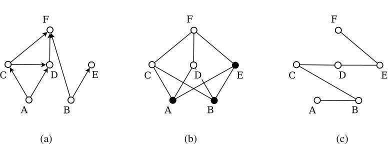
(a) (b) (c)
Figure 1: Three binary relations on the set{A,B,C,D,E,F}. (a) A DAG. (b) A Hasse diagram of a partial order compatible with the DAG. The partial order has12ideals, namely∅,{A}, {B},{A,B},{A,B,C},{A,B,D},{A,B,E},{A,B,C,D},{A,B,C,E},{A,B,D,E}, {A,B,C,D,E}, and{A,B,C,D,E,F}. One of the ideals is marked by black dots. (c) A Hasse diagram of a linear order that is an extension (superset) of both the DAG and the partial order.
called order ideals or downsets. We will show that, when maximizing a decomposable scoring function over DAGs that are compatible with a given a partial order, the basic dynamic programming algorithm can be trimmed to run only across the ideals. We illustrate this soon in Example 2 and give a general treatment in Sections 5.2 and 5.3.
Definition 8 (ideal) LetPbe a partial order onM. A subsetI ofMis called anidealofP ify∈I andxy∈P imply thatx∈I. We denote the set of all ideals ofPbyI(P).
Figure 1 illustrates some of the above defined concepts. Note that we visualize a partially ordered set(M, P)by itstransitive reduction, that is, the graph obtained by removing fromP all pairsxy for whichx=y or there exist az that is larger than x and smaller than y. We draw a transitive reduction on the plane using a Hasse diagram: a pairxyin the reduction corresponds to a line segment such thatxis positioned below or to the left ofy.
the partial order of size5. Continuing the same reasoning to smaller subproblems shows that it is sufficient to tabulate the optimal scores (DAGs) for the ideals of the partial order.
We will work with collections of partial orders that share the same ground set. We call such a collection apartial order systemon the ground set, orPOSfor short. Our interest is particularly in partial order systems that exhibit sufficient diversity so as to “cover” all linear orders on the ground set. This idea is formalized in the following:
Definition 9 (cover) A POS P on M is said to be a cover onM if any linear order on M is an extension of at least one partial order inP.
An extreme example of a cover on a ground setM is the collection{T}formed by the trivial orderT on M. At the other extreme we have the cover that consists of all linear orders onM. For yet another example, consider the three partial orders defined byP={AA,BB,CC,AB,AC}, Q={AA,BB,CC,BA,BC}, andR={AA,BB,CC,CA,CB}. We see that the system{P, Q, R} is a cover on the ground set{A,B,C}.
5.2 Dynamic Programming: First Phase
We aim at an algorithm that maximizesf(A)over all DAGs A on the node setN subject to the constraint thatAis compatible with a given partial orderP. In this subsection, we modify the first phase of the basic dynamic programming algorithm, described in Section 2.2, accordingly. In the next subsection, we will modify the second phase.
Recall that in the first phase, the task is to compute the valuesfˆv(Y)for all nodesvand node subsetsY ⊆N\ {v}. However, it turns out that, in the second phase, we need these values only for the idealsY of the given partial orderP. This gives us an opportunity to save space, provided that we have an appropriate “sparse” variant of the recurrence of Lemma 3 at hand. Next we present such a variant.
Our key insight is the following simple observation concerning collections of subsets. We leave the proof to the reader.
Lemma 10 LetXandY be sets withX⊆Y. Let
A= [X, Y] and B={Z⊆Y :x6∈Zfor somex∈X}.
Then (i)2Y =A ∪ Band (ii)B=S
x∈X2Y\{x}.
In terms of the set functionsfv andfˆv, for an arbitraryv, Lemma 10 amounts to the following generalization of Lemma 3 (one obtains Lemma 3 atX=Y):
Lemma 11 LetXandY be subsets ofN\ {v}withX⊆Y. Then
ˆ
fv(Y) = max
n
max
X⊆Z⊆Yfv(Z),maxu∈X
ˆ
fv(Y \ {u})
o
.
ABCD
ABC ABD ACD BCD
AB AC BC AD BD CD
A B C D
∅
Figure 2: Tails of the ideals{A,B,C}and{A,B,C,D}of the partial order of Figure 1(b), marked in black and gray, respectively, on the subset lattice of{A,B,C,D}. An interval from one set to another consists of the sets that are along a shortest path between the two sets in a Hasse diagram of the lattice. For example, the interval
{C},{A,B,C}
consists of the sets{C},{A,C},{B,C}, and{A,B,C}. In the figure, each subset is referred to by a sequence of its elements.
Lemma 11 leaves us the freedom to choose a suitable node subsetXfor each set of interestY. For this choice, we make use of the fact that in the second phase of dynamic programming, as it will turn out in the next subsection, we need the valuesfˆv(Y)only for setsY that are ideals ofP. Thus, our goal is to chooseXsuch thatY\ {u} ∈ I(P)for allu∈X. To this end, we letXconsist of all such nodes inY that have no larger node inY (w.r.t.P). Accordingly, forY ∈ I(P)define
ˇ
Y ={u∈Y :uv6∈P for allv∈Y\ {u}}.
Furthermore, define thetailofY as the interval
TY = [ ˇY , Y] ;
see Figure 2 for an illustration. By lettingX= ˇY and noting thatfv(Z) =−∞forZ6∈ Fv, we may rephrase the equation in Lemma 11 as
ˆ
fv(Y) = max
n
max
Z∈TY∩Fv
fv(Z),max u∈Yˇ
ˆ
fv(Y \ {u})
o
. (4)
The next two lemmas show thatYˇ indeed has the desired property (in a maximal sense) and that the tails of different idealsY are pairwise disjoint and thus optimally cover the subsets ofN.
Proof “If”: Letu∈Yˇ. Let st∈P. By the definition ofI(P)we need to show thatt∈Y \ {u} impliess∈Y \ {u}. So, supposet∈Y\ {u}, hencet∈Y. Now, sinceY ∈ I(P), we must have s∈Y. It remains to show thats6=u. But this holds becauseut6∈P by the definition ofYˇ.
“Only if”: Let u6∈Yˇ. Then we have uv ∈P for somev∈Y \ {u}. But u6∈Y \ {u} and v∈Y\ {u}, implyingY\ {u} 6∈ I(P)by the definition ofI(P).
Lemma 13 LetY andY′ be distinct ideals ofP. Then the tails ofY andY′ are disjoint.
Proof The lemma states that there does not exist any nonemptyZsuch thatZ∈ TY ∩TY′. Suppose
the contrary thatZ∈ TY ∩ TY′. By symmetry we may assume thatY\Y′ contains an elementw.
Thusw6∈Z, because Z⊆Y′. Because Yˇ ⊆Z, we havew6∈Yˇ. By the definition of Yˇ we con-clude that for everyu∈Y \Yˇ there existsv∈Yˇ such thatuv∈P. Therefore, in particular there existsv∈Yˇ such thatwv∈P. Sincew /∈Y′ andY′ is an ideal of P it follows by definition of an ideal thatv /∈Y′. On the other hand,v∈Yˇ andYˇ⊆Z⊆Y′implies thatv∈Y′: contradiction.
We we will use these lemmas in Section 5.4 to perform the recurrence of Lemma 11 over the ideals of the partial order and their tails.
5.3 Dynamic Programming: Second Phase
Recall that the second phase of the basic dynamic programming algorithm is captured by the recur-rence (1), which concerns all subsets ofN that can begin some linear order onN, that is, all the2n subsets. Now that we restrict our attention to DAGs that are compatible with the given partial order P, we may restrict the recurrence to only those sets that can begin some linear extension ofP, that is, to the ideals ofP. Formally, define the functiongP bygP(∅) = 0and for nonemptyY ∈ I(P) recursively:
gP(Y) = max
v∈Y Y\{v}∈I(P)
n
gP(Y\ {v}) + ˆfv(Y\ {v})
o
. (5)
We can show thatgP(N)equals the maximum score over the DAGs compatible withP:
Lemma 14 LetP be a partial order onN. Then
gP(N) = max{f(A) :Ais compatible withP}.
Furthermore, ifP is a cover onN, then
max
P∈Pg
P(N) = max A f(A),
whereAruns through all DAGs onN.
Proof LetP be a partial order onN. For any subsetY ⊆N denote byP[Y]the induced partial order{xy∈P:x, y∈Y}. We show by induction on the size ofY thatgP(Y)equals the maximum scoref(A′)over the DAGsA′⊆Y ×Y compatible withP[Y], assumingY is an ideal ofP. Here the scoref(A′)is naturally defined asP
For the base case, consider an arbitrary singleton {v} ∈ I(P). Clearly, there is exactly one DAGA′on{v}and it is compatible withP[{v}] ={vv}; the score of the DAG isf(A′) =fv(∅) =
ˆ
fv(∅). This is precisely what the recurrence (5) gives, asgP(∅) = 0.
Suppose then that the recurrence (5) holds for all proper subsets of a subsetY ⊆N. Without any loss of generality, we assumeY =N for notational convenience. Now, write
max
Ais compatible withPf(A) = maxL⊇PmaxA⊆L
X
v∈N fv(Av)
= max
L⊇P
X
v∈N
max
Av⊆Lv
fv(Av)
= max
L⊇P
X
v∈N
ˆ fv(Lv)
= max
v∈N
n
ˆ
fv(N\ {v}) + max L′⊇P[N\{v}]
X
u∈N\{v} ˆ fu(L′u)
o
= max
v∈N
n
ˆ
fv(N\ {v}) +gP[N\{v}](N\ {v})
o
.
HereLandL′ run trough the respective linear extensions andAthrough the DAGs satisfying the mentioned condition. The first identity holds by the definition of compatibility and the decompos-ability of the scoring functionf; the second one by the distributive law; the third one by the defini-tion offˆv; the fourth one because addition distributes over maximization and the fact that some node vis the last one in the linear orderLand that the induced linear orderL′on the remaining nodes is an extension of the induced partial orderP[N\ {v}]; the fifth one by the induction assumption (and the third identity). Finally, it suffices to notice thatgP(Y) =gP[Y](Y)forY ∈ I(P), since clearly
a subsetXofY is an ideal ofP if and only ifXis an ideal ofP[Y].
For the second statement, it suffices to observe that
max
P∈PmaxL⊇P
X
v∈N
ˆ
fv(Lv) = max L
X
v∈N
ˆ
fv(Lv) = max A f(A),
sinceP is a cover onN.
5.4 Dynamic Programming: First and Second Phase Merged
We now merge the ingredients given in the previous two subsections into an algorithm for evaluating gP using the recurrence (5) and Lemma 11, for a fixedP∈ P. In Algorithm 1 below,gP[Y]and
ˆ
Algorithm 1:
1. LetgP[∅]←0.
2. For eachv∈N, letfˆv[∅]←fv(∅).
3. For each nonemptyY ∈ I(P), in increasing order of cardinality:
(a) let
gP[Y]←max
v∈Yˇ
n
gP[Y\ {v}] + ˆfv[Y \ {v}]
o
;
(b) for eachv∈Y, letfˆv[Y]be the larger of
max
Z∈TY∩Fv
fv(Z) and max u∈Yˇ
ˆ
fv[Y\ {u}].
Lemma 15 Algorithm 1 correctly computesgP, that is,gP[Y] =gP(Y)for allY ∈ I(P).
Proof Observe first that the algorithm correctly computes fˆv for each v∈N, that is, after the execution of the algorithm we havefˆv[Y] = ˆfv(Y)for allv∈Y ∈ I(P). To this end, it suffices to note that step 3(b) implements the recurrence of Lemma 11 as rephrased in (4).
Then notice that step 3(a) implements the recurrence (5). Indeed, by Lemma 12, the condition “v∈Y andY \ {v} ∈ I(P)” of (5) is equivalent to “v∈Yˇ” of step 3(a), given that Y ∈ I(P) (guaranteed in step 3). This completes the proof.
To solve the OBN problem it suffices to run Algorithm 1 for every partial order in a system that is a cover onN. The appropriate partial order system of course varies with the problem instance, particularly with the number of nodesn. In the following statement of the time and space complexity of OBN, we do not fix any particular way to choose and construct the needed partial order system, but we simply refer to any appropriate system. Thus, the complexity results are nonuniform with this respect.
Theorem 16 (main) OBN can be solved in O P
P∈P(|I(P)| + F)
n2
time and O
maxP∈P|I(P)|+F nn space, assuming P is a cover of N and each Fv is downward closed and of size at mostF.
Proof By Lemmas 14 and 15, it suffices to run Algorithm 1 for eachP∈ P.
The time requirement of Algorithm 1 is dominated by steps 3(a) and 3(b). Given Y, the set ˇ
Y can be constructed in timeO(n2)by removing from Y each element that is not maximal inY. Thus, the contribution of step 3(a) in the total time requirement isO(|I(P)|n2).
We then analyze the time requirement of step 3(b), for fixed v. By Proposition 2, the maxi-mization of the local scores overTY ∩ Fv can be done inO(|TY ∩ Fv|n) time. By Lemma 13 the collections TY ∩ Fv are disjoint for different Y ∈ I(P). Thus the total contribution to the time requirement is proportional to|Fv| ≤F, for eachv. Because step 3(b) is executed|I(P)|times, the total time requirement of step 3(b) isO(|I(P)|n2+F n2). Combining the time bounds of steps 3(a) and 3(b) and summing over all members ofPyields the claimed boundO P
P∈P|I(P)|+F
n2
The space requirement for a fixed partial orderPisO(|I(P)|n), since by Lemma 12 the values gP[Y]andfˆv[Y]are only needed forY ∈ I(P). In addition, storing the local scores requiresO(F n) space for each nodev. Therefore, the total space requirement isO
maxP∈P|I(P)|+F nn.
Remark 17 Like in the basic DP algorithm, step 3 of Algorithm 1 can be implemented so that, compared to the bound in Theorem 16, a space saving proportional to√nis obtained.
5.5 Notes
We end this section with a couple of remarks on the general partial order approach.
The results in this section apply to any POS that is a cover on the node set. However, they do not tell us how to choose a POS that yields, in some sense, the most efficient tradeoff between space and time. Ideally, we would like to have a scheme that given a space bound as a function of the number of nodes n, saysn, gives us a POS Pn such that the space requirement implied byPn isO(sn) while the time requirement bound is minimized. Unfortunately, designing such an optimal scheme seems difficult due to the combinatorial challenge of simultaneously controlling the required cov-ering property of the partial order system and the number of ideals of the members of the system. Note that both counting the linear extensions and the ideals of a given partial order are #P-hard com-putational problems (Brightwell and Winkler, 1991; Provan and Ball, 1983), suggesting that their mathematical analysis is also not easy. In the next section we give a partial and practical solution to this issue by studying a subclass of series-parallel partial orders, which enables a derivation of concrete, quantitative space-time tradeoff results.
As another remark, we note that the algorithms can be easily parallelized onto|P|processors, each with its own memory, with negligible communication costs. This is in sharp contrast with the basic dynamic programming algorithm that does not enable such large-scale parallelization. We discuss the recent work by Tamada et al. (2011) in this light in Section 7. The ease of the paral-lelization stems from the fact that dynamic programming over the ideals can be done independently for each partial orderP inP. More precisely, each processor gets a dedicated partial orderP (and the local scores) as input and outputs the score gP(N) and a respective DAG. It then remains to communicate these outputs to a central unit that chooses an optimal one among them.
6. Bucket Order Schemes
To apply the partial order approach in practice, it is essential to find partial order systems that pro-vide a good tradeoff between time and space requirements. This section concentrates on a class of partial orders we callparallel bucket orders, which turn out to be relatively easy to analyze and seem to yield good tradeoff in practice. They also subsume, for instance, the two-bucket construction of Section 3.
6.1 Bucket Orders and Reorderings
read-ily extend to any finite number of partial orders. Because the series composition operation is not commutative, it is, of course, applied to a sequence of partial orders. Aseries-parallelpartial order is defined recursively: a partial order is a series-parallel partial order if it is either a singleton order or a parallel or series composition of two or more series-parallel partial orders. For example, the partial order{AA,BB,CC,AB,AC}is a series composition of{AA}and{BB,CC}, of which the former is a singleton order and the latter is a parallel composition of two singleton orders. Note that any trivial order is a parallel composition of singleton orders.
We study two special classes of series-parallel partial orders, namely bucket orders and parallel bucket orders. A bucket order is a series composition of the trivial orders on some ground sets B1, B2, . . . , Bℓ, calledbuckets. The bucket order is said to be oflengthℓandtype|B1| ∗ |B2| ∗ ··· ∗
|Bℓ|. We may denote the bucket order byB1B2···Bℓ. For instance, the series-parallel partial order in the previous paragraph is a bucket order{A}{B,C}, thus of length two and type1∗2. Likewise, the partial order in Figure 1(b) is a bucket order of length three and type2∗3∗1, the trivial order on some ground setM is of length one and type|M|, and a linear order onM is of length|M|and type1∗1∗ ··· ∗1.
By taking a parallel composition of some number of bucket orders we obtain aparallel bucket order. Note that the same parallel bucket order may be obtained by different collections of bucket orders. It is, however, easy to observe that for each parallel bucket order P there is a unique collection of bucket orders P1, P2, . . . , Pp, called the bucket orders ofP, such that their parallel composition isP and they are the connected components ofP.
The following lemma states a well-known result concerning the number of ideals of a series-parallel partial order (see, for example, Steiner’s article, 1990, and references therein).
Lemma 18 LetP1andP2be partial orders on disjoint ground sets. Then (i) the series composition
ofP1 andP2 has|I(P1)|+|I(P2)| −1ideals and (ii) the parallel composition ofP1 andP2 has
|I(P1)||I(P2)|ideals.
The next two lemmas state the number of ideals of a parallel bucket order.
Lemma 19 Let B be a bucket order B1B2. . . Bℓ. Then the number of ideals of B is given by |I(B)|= 1−ℓ+ 2|B1|+ 2|B2|+···+ 2|Bℓ|.
Proof Any singleton order has two ideals, namely the empty set and the ground set. Thus, by Lemma 18(ii), the trivial order on the bucketBihas2|Bi|ideals, for eachi. Hence, by Lemma 18(i), Bhas1−ℓ+ 2|B1|+ 2|B2|+···+ 2|Bℓ|ideals.
We note that the order of buckets does not affect the number of ideals.
Lemma 20 LetP be the parallel composition of bucket ordersP1, P2, . . . , Pp. Then the number of ideals ofP is given by|I(P)|=|I(P1)||I(P2)|···|I(Pp)|.
Proof Follows immediately from Lemma 18(ii).
Definition 21 (reordering) We say two bucket orders arereorderingsof each other if they have the same ground set and they are of the same type. Furthermore, we say two parallel bucket orders are reorderingsof each other if their bucket orders can be labelled asP1, P2, . . . , PpandQ1, Q2, . . . , Qp, respectively, such thatPiis a reordering ofQi for eachi. We denote the collection of reorderings of a parallel bucket orderP byR(P).
We note that two bucket orders are reorderings of each other if and only if they are automorphic to each other. However, this equivalence does not hold for parallel bucket orders in general, for reordering only allows shuffling within each bucket order, but not between different bucket orders.
It can be shown thatR(P)is a cover on the ground set ofP. The proof below slightly simplifies the one we have given earlier (Koivisto and Parviainen, 2010, Theorem 3.1).
Theorem 22 LetP be a parallel composition of bucket orders. ThenR(P)is a cover on the ground set ofP.
Proof LetLbe a linear order onM. It suffices to construct a parallel bucket orderQ∈ R(P)such thatLis an extension ofQ. To this end, letP1, P2, . . . , Ppbe the bucket orders ofP, with respective ground setsM1, M2, . . . , Mp. For eachi= 1,2, . . . , p, construct a bucket orderQionMias follows: Letm1∗m2··· ∗mℓ be the type of Pi. LetL′ be the induced orderL[Mi]. Observe that L′ is a linear order. Now, putQi=C1C2···CℓwhereC1consists of the firstm1 elements in the orderL′,
C2 consists of the nextm2 elements in the order, and so forth. Observe thatL′ is an extension of
Qi and thatQi is a reordering ofPi. Finally, letQbe the parallel composition ofQ1, Q2, . . . , Qp. Clearly,Q∈ R(P). To complete the proof, note thatLis an extension ofQ, sincexy∈Qimplies xy∈Qifor somei, whencexy∈L[Mi]⊆L.
When P is a parallel composition of p bucket orders, each of type b1∗b2∗ ··· ∗bℓ, we find it convenient to denote the POSR(P) by (b1∗b2∗ ··· ∗bℓ)p. This notation is explicit about the combinatorial structure of the POS, while it ignores the arbitrariness of the labeling of the ground set. When the size of the ground set, n, is clear from the context, we may extend the notation (b1∗b2∗ ··· ∗bℓ)p to refer to a systemR(P), whereP is a parallel composition ofpbucket orders of typeb1∗b2∗ ··· ∗bℓand one trivial order on the remainingn−p(b1+b2+···+bℓ)elements. It is instructive to notice that a POS(b1∗b2∗ ··· ∗bℓ)p consists of b1b1+bb22+······+bℓbℓ
p
different partial
orders, since any bucket order of typeb1∗b2∗ ··· ∗bℓhas exactly b1b1+bb22+······+bℓbℓ
=(b1+b2+···+bℓ)!
b1!b2!···bℓ!
different reorderings.
For an illustration of these concepts, consider a node set N ={A,B,C,D,E,F,G,H} parti-tioned intoN1={A,B,C,D,E,F}andN2={G,H}. Let the bucket order onN1be the one shown
in Figure 1(b), denoted asP1, and let the bucket order onN2be the trivial order{GG,HH}, denoted
asP2. Now the reorderings of the parallel composition ofP1 andP2 form a POS(2∗3∗1)1. By
Lemma 19,P1has1−3 + 22+ 23+ 21= 12ideals andP2has1−1 + 22= 4ideals. By Lemma 20,
the total number of ideals of the parallel composition ofP1andP2is12×4 = 48. The number of
the partial orders in(2∗3∗1)1 is 2 63 11
= 60.
6.2 Bucket Order Schemes
that can take different values, we refer to the implied family of partial order systems as abucket order scheme. Furthermore, we denote the scheme simply by the expression (b1∗b2∗ ··· ∗bℓ)p, where the parameters and their ranges are assumed to understood from the context. For instance, we may talk about the scheme(5∗5)p, understanding thatptakes values over its natural range, that is,p= 1,2, . . . ,⌊n/(5 + 5)⌋. Another example of a bucket order scheme is thetwo-bucket schemeof Section 3, which corresponds to partial order systems(s∗(n−s))1, withstreated as the parameter. Other examples are thepairwise scheme, corresponding to systems(1∗1)p, withpas the parameter, and thegeneralized two-bucket scheme defined by the systems(⌈m/2⌉ ∗ ⌊m/2⌋)⌊n/m⌋, withmas the parameter.
Via Theorem 16, any fixed bucket order scheme implies parameterized time and space complex-ity bounds for the OBN problem. Moreover, one scheme may dominate another scheme in the sense of yielding an equal or smaller time bound at any space bound. While it is currently an open prob-lem to characterize bucket order schemes that dominate all other bucket order schemes, our analysis of the so-called space-time product (Koivisto and Parviainen, 2010) suggests that the most efficient trade-off is achieved with the bucket order scheme(⌈m/2⌉,⌊m/2⌋)p. The scheme guarantees that the product of the time and space requirements scales roughly asCn, whereCequals4or is slightly below4depending on the space bound. If some other scheme resulted in a significantly faster algo-rithm at any space bound, then that scheme would make a new record also in terms of the space-time product, albeit possibly at a single point. Our prior study (Koivisto and Parviainen, 2010) shows that no such scheme exists among bucket order schemes. When measured by the space-time prod-uct, the tradeoff of the scheme(⌈m/2⌉,⌊m/2⌋)pslowly improves whenmincreases, untilm= 26, after which the tradeoff starts slowly getting worse. We next examine this scheme in more detail focusing on the range2≤m≤26. See Figure 4 (in Section 7) for the tradeoff curve.
6.3 Practical Bucket Order Schemes
A partial order system (⌈m/2⌉ ∗ ⌊m/2⌋)p consists of ⌊m/m2⌋p
partial orders, each having 2n−mp(2⌊m/2⌋+ 2⌈m/2⌉−1)p ideals. Plugging these numbers into Theorem 16 gives us the fol-lowing time and space bounds.
Corollary 23 OBN can be solved inO m
⌊m/2⌋
p
(I+F)
n2
time andO [I+F n]n
space, where I= 2n−mp(2⌊m/2⌋+ 2⌈m/2⌉−1)p, for anym= 2, . . . , nandp= 0, . . . ,⌊n/m⌋, assuming eachFv is downward closed and of size at mostF.
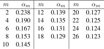
We observe that the number of ideals, I, dominates both the time and space requirements as long as the input size, roughlyF, is not too large. Note that pruning the parent sets affectsFbut has no effect onI. Since in our case,I usually grows exponentially inn, exponentially large families of potential parent sets can be handled with negligible extra cost. To investigate this issue more carefully, we focus on the case where each node is allowed to have at mostk=αnparents, with someslopeα≤1/2. How large can the slopeαbe, yet guaranteeing that the size of the input does not dominate the time and space requirements? Recall that now the termF nin the space bound can be replaced byF.
largest slope by αm, as follows. It is well-known that Pαi=0mn ni
, an upper bound for the num-ber of potential parent sets per node, is at most2H(αm)n
, where H is the binary entropy function (for a proof, see for example Flum and Grohe (2006, p. 427)). On the other hand, every par-tial order in the system (m/2∗m/2)n/m has ((2m/2+1−1)1/m)n ideals. Thus, the number of ideals dominates the space and time requirements if2H(αm)n
≤((2m/2+1−1)1/m)n, equivalently, H(αm)≤1/mlog2(2m/2+1−1). Solving this inequality numerically gives us a boundαm. Table 1 shows theαmfor each evenm≤26.
m αm m αm m αm 2 0.238 12 0.139 20 0.127 4 0.190 14 0.135 22 0.125 6 0.167 16 0.131 24 0.124 8 0.153 18 0.129 26 0.123 10 0.145
Table 1: Bounds on the maximum indegree slopes for the scheme(m/2∗m/2)n/m.
Since the partial orders in(m/2∗m/2)n/mhave as many or fewer ideals than the partial orders in(m/2∗m/2)p, forp≤n/m, we have the following characterization.
Corollary 24 OBN can be solved in O m/m2
2n−mp(2m/2+1 − 1)p
n2
time and O 2n−mp(2m/2+1−1)pn
space for any p = 0,1,2, . . . ,⌊n/m⌋ and m = 2,4,6, . . .26, pro-vided that each node has at mostαmnparents, withαmas given in Table 1.
For example, the maximum indegree in30-node DAGs can be set to⌊0.238×30⌋= 7in the pairwise scheme(1∗1)pand to⌊0.139×30⌋= 4in the scheme(6∗6)p. A larger maximum indegree may render the input size dominate the number of ideals in the time and space requirements. In the next subsection we provide some empirical results, which suggest that the bounds in Table 1 are only slightly conservative.
6.4 Empirical Results
We have implemented the presented algorithm in the C++language into a publicly available com-puter program BOSON (Bucket Order Scheme for Optimal Networks).4 As the implementation is not fully optimized, the empirical results reported below should be viewed rather as a proof of concept.5 We tested our implementation varying the number of nodesn, bucket order sizesm, and the number of parallel bucket ordersp. The experiments were run on Intel Xeon R5540 processors, each with 32 GB of RAM.
We examined the running time for the limit of 16 GB of memory, letting the number of nodes nvary from25to34, with maximum indegree set to 3. The local scores were taken as given, so
4. BOSON is available atwww.csc.kth.se/˜pekkapa/code/boson-1.0.tar.gz.