How to Explain Individual Classification Decisions
David Baehrens∗ [email protected]
Timon Schroeter∗ [email protected]
Technische Universit¨at Berlin Franklinstr. 28/29, FR 6-9 10587 Berlin, Germany
Stefan Harmeling∗ [email protected]
MPI for Biological Cybernetics Spemannstr. 38
72076 T¨ubingen, Germany
Motoaki Kawanabe† [email protected] Fraunhofer Institute FIRST.IDA
Kekulestr.7
12489 Berlin, Germany
Katja Hansen [email protected]
Klaus-Robert M ¨uller [email protected] Technische Universit¨at Berlin
Franklinstr. 28/29, FR 6-9 10587 Berlin, Germany
Editor: Carl Edward Rasmussen
Abstract
After building a classifier with modern tools of machine learning we typically have a black box at hand that is able to predict well for unseen data. Thus, we get an answer to the question what is the most likely label of a given unseen data point. However, most methods will provide no answer why the model predicted a particular label for a single instance and what features were most influential for that particular instance. The only method that is currently able to provide such explanations are decision trees. This paper proposes a procedure which (based on a set of assumptions) allows to explain the decisions of any classification method.
Keywords: explaining, nonlinear, black box model, kernel methods, Ames mutagenicity
1. Introduction
Automatic nonlinear classification is a common and powerful tool in data analysis. Machine learn-ing research has created methods that are practically useful and that can classify unseen data after being trained on a limited training set of labeled examples.
Nevertheless, most of the algorithms do not explain their decision. However in practical data analysis it is essential to obtain an instance-based explanation, that is, we would like to gain an
∗. The first three authors contributed equally.
understanding what input features made the nonlinear machine give its answer for each individual data point.
Typically, explanations are provided jointly for all instances of the training set, for example feature selection methods (including Automatic Relevance Determination) find out which inputs are salient for a good generalization (see Guyon and Elisseeff, 2003, for a review). While this can give a coarse impression about the global usefulness of each input dimension, it is still an ensemble view and does not provide an answer on an instance basis.1 In the neural network literature also solely an ensemble view was taken in algorithms like input pruning (e.g., Bishop, 1995; LeCun et al., 1998). The only classification that does provide individual explanations are decision trees (e.g., Hastie et al., 2001).
This paper proposes a simple framework that provides local explanation vectors applicable to any classification method in order to help understanding prediction results for single data instances. The local explanation yields the features relevant for the prediction at the very points of interest in the data space, and is able to spot local peculiarities that are neglected in the global view, for example, due to cancellation effects.
The paper is organized as follows: We define local explanation vectors as class probability gradi-ents in Section 2 and give an illustration for Gaussian Process Classification (GPC). Some methods output a prediction without a direct probability interpretation. For these we propose in Section 3 a way to estimate local explanations. In Section 4 we apply our methodology to learn distinguishing properties of Iris flowers by estimating explanation vectors for a k-NN classifier applied to the clas-sic Iris data set. In Section 5 we discuss how our approach applied to a SVM classifier allows us to explain how digit “2” is distinguished from digit “8” in the USPS data set. In Section 6 we focus on a more real-world application scenario where the proposed explanation capabilities prove useful in drug discovery: Human experts regularly decide how to modify existing lead compounds in order to obtain new compounds with improved properties. Models capable of explaining predictions can help in the process of choosing promising modifications. Our automatically generated explanations match with chemical domain knowledge about toxifying functional groups of the compounds in question. Section 7 contrasts our approach with related work and Section 8 discusses characteristic properties and limitations of our approach, before we conclude the paper in Section 9.
2. Definitions of Explanation Vectors
In this Section we will give definitions for our approach of local explanation vectors in the classi-fication setting. We start with a theoretical definition for multi-class Bayes classiclassi-fication and then give a specialized definition being more practical for the binary case.
For the multi-class case, suppose we are given data points x1, . . . ,xn∈ℜdwith labels y1, . . . ,yn∈
{1, . . . ,C}and we intend to learn a function that predicts the labels of unlabeled data points.
As-suming that the data is IID-sampled from some unknown joint distribution P(X,Y), we define the
Bayes classifier,
g∗(x) =arg min
c∈{1,...,C}P(Y6=c|X=x)
which is optimal for the 0-1 loss function (see Devroye et al., 1996).
For the Bayes classifier we define the explanation vector of a data point x0to be the derivative with respect to x at x=x0of the conditional probability of Y6=g∗(x0)given X=x, or formally, Definition 1
ζ(x0):= ∂
∂xP(Y6=g
∗(x)|X=x)
x=x0
.
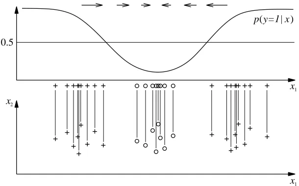
Note thatζ(x0)is a d-dimensional vector just like x0is. The classifier g∗partitions the data spaceℜd into up to C parts on which g∗is constant. We assume that the conditional distribution P(Y=c|X= x)is first-order differentiable w.r.t. x for all classes c and over the entire input space. For instance, this assumption holds if P(X=x|Y=c)is for all c first-order differentiable in x and the supports of the class densities overlap around the border for all neighboring pairs in the partition by the Bayes classifier. The vectorζ(x0)defines on each of those parts a vector field that characterizes the flow away from the corresponding class. Thus entries inζ(x0)with large absolute values highlight features that will influence the class label decision of x0. A positive sign of such an entry implies that increasing that feature would lower the probability that x0 is assigned to g∗(x0). Ignoring the orientations of the explanation vectors,ζ forms a continuously changing (orientation-less) vector field along which the class labels change. This vector field lets us locally understand the Bayes classifier.
We remark that ζ(x0) becomes a zero vector, for example, when P(Y6=g∗(x)|X=x)|x=x0 is
equal to one in some neighborhood of x0. Our explanation vector fits well to classifiers where the conditional distribution P(Y =c|X =x) is usually not completely flat in some regions. In the case of deterministic classifiers, despite of this issue, Parzen window estimators with appropriate widths (Section 3) can provide meaningful explanation vectors for many samples in practice (see also Section 8).
In the case of binary classification we directly define local explanation vectors as local gradients of the probability function p(x) =P(Y =1|X =x)of the learned model for the positive class.
For a probability function p : ℜd →[0,1] of a classification model learned from examples
{(x1,y1), . . . ,(xn,yn)} ∈ℜd× {−1,+1}the explanation vector for a classified test point x0 is the
local gradient of p at x0:
Definition 2
ηp(x0):=∇p(x)|x=x0.
By this definition the explanationηis again a d-dimensional vector just like the test point x0is. The sign of each of its individual entries indicates whether the prediction would increase or decrease when the corresponding feature of x0is increased locally and each entry’s absolute value gives the amount of influence in the change in prediction. The vectorηgives the direction of the steepest ascent from the test point to higher probabilities for the positive class. For binary classification the negative version−ηp(x0)indicates the changes in features needed to increase the probability for
For an example we apply Definition 2 to model predictions learned by Gaussian Process Clas-sification (GPC), see Rasmussen and Williams (2006). GPC is used here for three reasons:
(i) In our real-world application we are interested in classifying data from drug discovery, which is an area where Gaussian processes have proven to show state-of-the-art performance, see, for example, Obrezanova and Segall (2010), Obrezanova et al., Schroeter et al. (2007c), Schroeter et al. (2007a), Schroeter et al. (2007b), Schwaighofer et al. (2007), Schwaighofer et al. (2008) and Obrezanova et al. (2008). It is natural to expect a model with high prediction accuracy on a complex problem to capture relevant structure of the data which is worth explaining and may give domain specific insights in addition to the values predicted. For an evaluation of the explaining capabilities of our approach on a complex problem from chemoinformatics see Section 6.
(ii) GPC does model the class probability function used in Definition 2 directly. For other classi-fication methods such as Support Vector Machines that do not provide a probability function as its output we give an example for an estimation method starting from Definition 1 in Section 3. (iii) The local gradients of the probability function can be calculated analytically for differentiable kernels as we discuss next.
Let f(x) =∑ni=1αik(x,xi)be a Gaussian Process (GP) model trained on sample points x1, . . . ,xn∈
ℜdwhere k is a kernel function andα
iare the learned weights of each sample point. For a test point
x0∈ℜd let varf(x0) be the variance of f(x0) under the GP posterior of f . Because the posterior
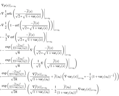
cannot be calculated analytically for GP classification models, we used an approximation by ex-pectation propagation (EP) (Kuss and Ramussen, 2005). In the case of the probit likelihood term defined by the error function, the probability for being of the positive class p(x0)can be computed easily from this approximated posterior as
p(x0) =1 2erfc
−f(x0) √
2·p1+varf(x0)
!
,
where erfc denotes the complementary error function (see Equation 6 in Schwaighofer et al., 2008). Then the local gradient of p(x0)is given by2
∇p(x)|x=x0=
exp2(1−+fvar(x0)2
f(x0))
√2π p∇f(x)|x=x0 1+varf(x0)
−1 2
f(x0) (1+varf(x0))
3 2
∇varf(x)|x=x0
!
. (1)
As a kernel function choose, for example, the RBF-kernel k(x0,x1) =exp(−w(x0−x1)2), which has the derivative(∂/∂x0,j)k(x0,x1) =−2w exp(−w(x0−x1)2)(x0,j−x1,j)for j∈ {1, . . . ,d}. Then the
elements of the local gradient∇f(x)|x=x0 are
∂f ∂x0,j
=−2w
n
∑
i=1
αiexp(−w(x0−xi)2)(x0,j−xi,j) for j∈ {1, . . . ,d}.
For varf(x0) =k(x0,x0)−kT∗(K+Σ)−1k∗the derivative is given by3
∇varf(x)|x=x0=
∂varf
∂x0,j
=
∂
∂x0,j
k(x0,x0)
−2∗kT∗(K+Σ)−1 ∂ ∂x0,j
k∗ for j∈ {1, . . . ,d}.
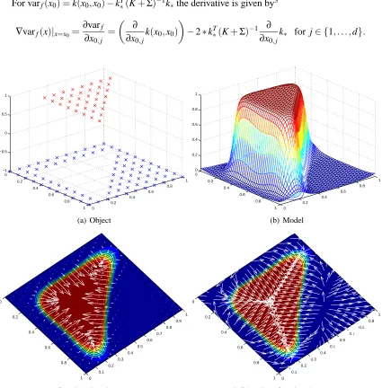
0 0.2 0.4 0.6 0.8 1 0 0.2 0.4 0.6 0.8 1 −1 −0.5 0 0.5 1 (a) Object 0 0.2 0.4 0.6 0.8 1 0 0.2 0.4 0.6 0.8 1 0 0.2 0.4 0.6 0.8 1 (b) Model 0 0.2 0.4 0.6 0.8 1 0 0.1 0.2 0.3 0.4 0.5 0.6 0.7 0.8 0.9 1
(c) Local explanation vectors
0 0.2 0.4 0.6 0.8 1 0 0.1 0.2 0.3 0.4 0.5 0.6 0.7 0.8 0.9 1
(d) Direction of explanation vectors
Figure 1: Explaining simple object classification with Gaussian Processes
Panel (a) of Figure 1 shows the training data of a simple object classification task and panel (b) shows the model learned using GPC.4The data is labeled−1 for the blue points and+1 for the red points. As illustrated in panel (b) the model is a probability function for the positive class which gives every data point a probability of being in this class. Panel (c) shows the probability gradient of the model together with the local gradient explanation vectors. Along the hypotenuse and at the corners of the triangle explanations from both features interact towards the triangle class while along
3. Here k∗= (k(x0,x1), . . . ,k(x0,xn))T is the evaluation of the kernel function between the test point x0 and every
training point. Σis the diagonal matrix of the variance parameter. For details see Rasmussen and Williams (2006, Chapter 3).
the edges the importance of one of the two feature dimensions dominates. At the transition from the negative to the positive class the length of the local gradient vectors represents the increased importance of the relevant features. In panel (d) we see that explanations close to the edges of the plot (especially in the right hand side corner) point away from the positive class. However, panel (c) shows that their magnitude is very small. For discussion of this issue see Section 8.
3. Estimating Explanation Vectors
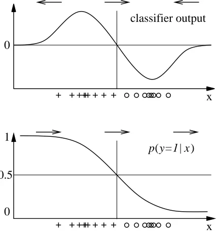
Several classification methods directly estimate the decision rule, which often has no interpretation as the probability function in terms of Definition 2. For example Support Vector Machines estimate a decision function of the form
f(x) =
n
∑
i=1
αik(xi,x) +b,
αi,b∈ℜ. Suppose we have two classes (each with one cluster) in one dimension (see Figure 2)
and train a SVM with RBF kernel. For points outside the data clusters f(x)tends to zero. Thus, the derivative of f(x)(shown as arrows above the curves) for points on the very left or on the very right side of the axis will point to the wrong side. In the following, we will explain how explanations can
0
x
p( | )y=1 x
1
0.5
0
x classifier output
Figure 2: Classifier output of an SVM (top) compared to p(y=1|x)(bottom).
be obtained for such classifiers.
In practice, we do not have access to the true underlying distribution P(X,Y). Consequently, we have no access to the Bayes classifier as defined in Section 2. Instead, we can apply sophis-ticated learning machinery like Support Vector Machines (Vapnik, 1995; Sch¨olkopf and Smola, 2002; M¨uller et al., 2001) that estimates some classifier g that tries to mimic g∗. For test data points
z1, . . . ,zm∈ℜd which are assumed to be sampled from the same unknown distribution as the
no access, we will define explanation vectors that help us understand the classifier g on the test data points.
Since we do not assume that we have access to some intermediate real-valued classifier output here (of which g might be a thresholded version and which further might not be an estimate of P(Y= c|X=x)), we suggest to approximate g by another classifier ˆg, the actual form of which resembles the Bayes classifier. There are several choices for ˆg, for example, GPC, logistic regression, and Parzen windows.5 In this paper we apply Parzen windows to the training points to estimate the weighted class densities P(Y=c)·P(X |Y=c), for the index set Ic={i|g(xi) =c}
ˆ
pσ(x,y=c) =1
ni
∑
∈Ickσ(x−xi) (2)and with kσ(z)being a Gaussian kernel kσ(z) =exp(−0.5 z⊤z/σ2)/√2πσ2(as always other kernels are also possible). This estimates P(Y=c|X=x)for all c,
ˆ
pσ(y=c|x) = pˆσ(x,y=c) ˆ
pσ(x,y=c) +pˆσ(x,y6=c)≈
∑i∈Ickσ(x−xi)
∑ikσ(x−xi)
(3)
and thus is an estimate of the Bayes classifier (that mimics g),
ˆ
gσ(x) =arg min
c∈{1,...,C}pˆσ(y6=c|x).
This approach has the advantage that we can use our estimated classifier g to generate any amount of labeled data for constructing ˆg. The single hyper-parameterσis chosen such that ˆg approximates g (which we want to explain), that is,
ˆ
σ:=arg min
σ
m
∑
j=1
Ig(zj)=6 gˆσ(zj) ,
where I{···}is the indicator function. σis assigned the constant value ˆσfrom here on and omitted as a subscript. For ˆg it is straightforward to define explanation vectors:
Definition 3
ˆ
ζ(z):= ∂
∂x pˆ(y6=g(z)|x)
x=z
=
∑i∈/Ig(z)k(z−xi)
∑i∈Ig(z)k(z−xi)(z−xi)
σ2 ∑n
i=1k(z−xi)
2
−
∑i∈/Ig(z)k(z−xi)(z−xi)
∑i∈Ig(z)k(z−xi)
σ2 ∑n
i=1k(z−xi)
2 .
This is easily derived using Equation (3) and the derivative of Equation (2), see Appendix A.3.1. Note that we use g instead of ˆg. This choice ensures that the orientation of ˆζ(z)fits to the labels assigned by g, which allows better interpretations.
In summary, we imitate the classifier g which we would like to explain locally by a Parzen window classifier ˆg that has the same form as the Bayes estimator and for which we can estimate the
explanation vectors using Definition 3. Practically there are some caveats: The mimicking classifier ˆ
g has to be estimated from g even in high dimensions; this needs to be done with care. However, in principle we have an arbitrary amount of training data available for constructing ˆg since we may use our estimated classifier g to generate labeled data.
4. Explaining Iris Flower Classification by k-Nearest Neighbors
The Iris flower data set (introduced in Fisher, 1936) describes 150 flowers from the genus Iris by four features: sepal length, sepal width, petal length, and petal width, all of which are easily measured properties of certain leaves of the corolla of the flower. There are three clusters in this data set that correspond to three different species: Iris setosa, Iris virginica, and Iris versicolor.
Let us consider the problem of classifying the data points of Iris versicolor (class 0) against the other two species (class 1). We applied standard classification machinery to this problem as follows:
• Class 0 consists of all examples of Iris versicolor.
• Class 1 consists of all examples of Iris setosa and Iris virginica.
• Randomly split 150 data points into 100 training and 50 test examples.
• Normalize training and test set using the mean and variance of the training set.
• Apply k-nearest neighbor classification with k=4 (chosen by leave-one-out cross-validation on the training data).
• Training error is 3% (i.e., 3 mistakes in 100).
• Test error is 8% (i.e., 4 mistakes in 50).
In order to estimate explanation vectors we mimic the classification results with a Parzen window classifier. The best fit (3% error) is obtained with a kernel width ofσ=0.26 (chosen by leave-one-out cross-validation on the training data).
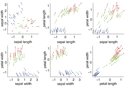
Since the explanation vectors live in the input space we can visualize them with scatter plots of the initially measured features. The resulting explanations (i.e., vectors) for the test set are shown in Figure 3. The blue markers correspond to explanation vectors of Iris setosa and the red markers correspond to those of of Iris virginica (both class 1). Both groups of markers point to the green markers of Iris versicolor. The most important feature is the combination of petal length and petal width (see the corresponding panel), the product of which corresponds roughly to the area of the petals. However, the resulting explanations for the two species in class 1 are different:
• Iris setosa (class 1) is different from Iris versicolor (class 0) because its petal area is smaller.
• Iris virginica (class 1) is different from Iris versicolor (class 0) because its petal area is larger.
Figure 3: Scatter plots of the explanation vectors for the test data. Shown are all explanation vectors for both classes: class 1 containing Iris setosa (shown in blue) and Iris virginica (shown in red) versus class 0 containing only the species Iris versicolor (shown in green). Note that the explanations why an Iris flower is not an Iris versicolor is different for Iris setosa and Iris virginica.
5. Explaining USPS Digit Classification by Support Vector Machine
We now apply the framework of estimating explanation vectors to a high dimensional data set, the USPS digits. The classification problem that we designed for illustration purposes is detailed in the following list:
• digits: 16×16 images that are reshaped to 256×1 dimensional column vectors
• classifier: SVM from Schwaighofer (2002) with RBF kernel widthσ=1 and regularization constant C=10 (chosen by grid search in cross-validation on the training data).
• training set: 47 “twos”, 53 “eights”; training error 0.00
• test set: 48 “twos”, 52 “eights”; test error 0.05
Figure 4: USPS digits (training set): “twos” (left) and “eights” (right) with correct classification. For each digit from left to right: (i) explanation vector (with black being negative, white being positive), (ii) the original digit, (iii-end) artificial digits along the explanation vector towards the other class.
fit was achieved. Figures 4 and 5 show our results. All parts show three examples per row. For each example we display from left to right: (i) the explanation vector, (ii) the original digit, (iii-end) artificial digits along the explanation vector towards the other class.6 These artificial digits should help to understand and interpret the explanation vector. Let us first have a look at the results on the training set:
Figure 4 (left panel): Let us focus on the top example framed in red. The line that forms the “two” is part of some “eight” from the data set. Thus the parts of the lines that are missing show up in the explanation vector: if the dark parts (which correspond to the missing lines) are added to the “two” digit then it will be classified as an “eight”. In other words, because of the lack of those parts the digit was classified as a “two” and not as an “eight”. A similar explanation holds for the middle example framed in red in the same Figure. Not all examples transform easily to “eights”: Besides adding parts of black lines, some existing black spots (that make the digit be a “two”) must be removed. This is reflected in the explanation vector by white spots/lines. The bottom “two”, framed in red, is actually a dash and is in the data set by mistake. However, its explanation vector shows nicely which parts have to be added and which have to be removed.
Figure 4 (right panel): We see similar results for the “eights” class. The explanation vectors again tell us how the “eights” have to change to become classified as “twos”. However, sometimes the transformation does not reach the “twos”. This is probably due to the fact that some of the “eights” are inside the cloud of “eights”.
On the test set the explanation vectors are not as pronounced as on the training set. However, they show similar tendencies:
Figure 5 (left panel): We see the correctly classified “twos”. Let’s focus on the example framed in red. Again the explanation vector shows us how to edit the image of the “two” to transform it into an “eights”, that is, exactly which parts of the digit were important for the classification result. For several other “twos” the explanation vectors do not directly lead to the “eights” but weight the different parts of the digits that were relevant for the classification.
Figure 5 (right panel): Similarly to the training data, we see that also these explanation vectors are not bringing all “eights” to “twos”. Their explanation vectors mainly suggest to remove most of the “eights” (black pixels) and add some black in the lower part (the light parts, which look like a white shadow).
Overall, the explanation vectors tell us how to edit our example digits to change the assigned class label. Hereby, we get a better understanding of the reasons why the chosen classifier classified the way it did.
6. Explaining Mutagenicity Classification by Gaussian Processes
In the following Section we describe an application of our local gradient explanation methodology to a complex real world data set. Our aim is to find structure specific to the problem domain that has not
been fed into training explicitly but is captured implicitly by the GPC model in the high-dimensional feature space used to determine its prediction. We investigate the task of predicting Ames mutagenic activity of chemical compounds. Not being mutagenic (i.e., not able to cause mutations in the DNA) is an important requirement for compounds under investigation in drug discovery and design. The Ames test (Ames et al., 1972) is a standard experimental setup for measuring mutagenicity. The following experiments are based on a set of Ames test results for 6512 chemical compounds that we published previously.7
GPC was applied as follows:
• Class 0 consists of non-mutagenic compounds.
• Class 1 consists of mutagenic compounds.
• Randomly split 6512 data points into 2000 training and 4512 test examples such that:
– The training set consists of equally many class 0 and class 1 examples.
– For the steroid compound class the balance in the training and test set is enforced.
• 10 additional random splits were investigated individually. This confirmed the results pre-sented below.
• Each example (chemical compound) is represented by a vector of counts of 142 molecular substructures calculated using the DRAGONsoftware (Todeschini et al., 2006).
• Normalize training and test set using the mean and variance of the training set.
• Apply GPC model with RBF kernel.
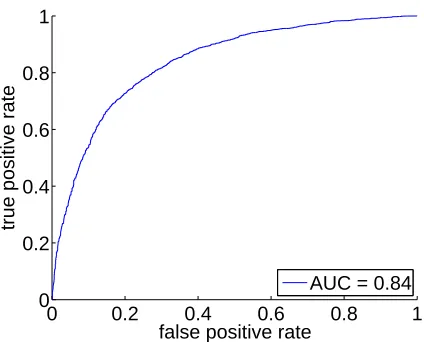
• Performance (84 % area under curve) confirms our previous results (Hansen et al., 2009). Error rates can be obtained from Figure 6.
Together with the prediction we calculated the explanation vector (as introduced in Definition 2) for each test point. The remainder of this Section is an evaluation of these local explanations.
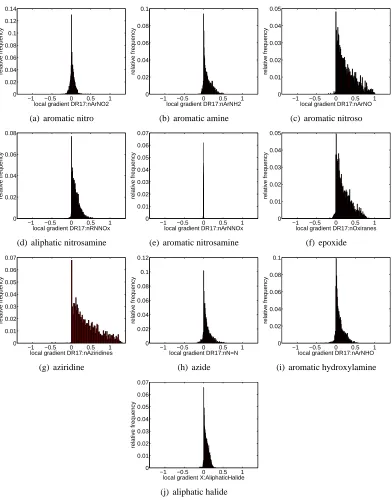
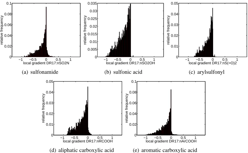
In Figures 7 and 8 we show the distribution of the local importance of selected features across the test set: For each input feature we generate a histogram of local importance values, as indicated by its corresponding entry in the explanation vector of each of the 4512 test compounds. The features examined in Figure 7 are counts of substructures known to cause mutagenicity. We show all approved “specific toxicophores” introduced by Kazius et al. (2005) that are also represented in the DRAGON set of features. The features shown in Figure 8 are known to detoxify certain toxicophores (again see Kazius et al., 2005). With the exception of 7(e) the toxicophores also have a toxifying influence according to our GPC prediction model. Feature 7(e) seems to be mostly irrelevant for the prediction of the GPC model on the test points. In contrast the detoxicophores show overall negative influence on the prediction outcome of the GPC model. Modifying the test compounds by adding toxicophores will increase the probability of being mutagenic as predicted by the GPC model while adding detoxicophores will decrease this predicted probability.
0 0.2 0.4 0.6 0.8 1 0
0.2 0.4 0.6 0.8 1
false positive rate
true positive rate
AUC = 0.84
Figure 6: Receiver operating characteristic curve of GPC model for mutagenicity prediction
We have seen that the conclusions drawn from our explanation vectors agree with established knowledge about toxicophores and detoxicophores. While this is reassuring, such a sanity check re-quired existing knowledge about which compounds are toxicophores and detoxicophores and which are not. Thus it is interesting to ask whether we also could have discovered that knowledge from the explanation vectors. To answer this question we ranked all 142 features by the means of their local gradients.8 Clear trends result: 9 out of 10 known toxicophores can be found close to the top of the list (mean rank of 19). The only exception (rank 81) is the aromatic nitrosamine feature.9 This trend is even stronger for the detoxicophores: The mean rank of these five features is 138 (out of 142), that is, they consistently exhibit the largest negative local gradients. Consequently, the established knowledge about toxicophores and detoxicophores could indeed have been discovered using our methodology.
In the following paragraph we will discuss steroids10as an example of an important compound class for which the meaning of features differs from this global trend, so that local explanation vectors are needed to correctly identify relevant features.
Figure 9 displays the difference in relevance of epoxide (a) and aliphatic nitrosamine (c) sub-structures for the predicted mutagenicity of steroids and non-steroid compounds. For compari-son we also show the distributions for compounds chosen at random from the test set (b,d). Each subfigure contains two measures of (dis-)similarity for each pair of distributions. The p-value of the Kolmogorov-Smirnoff test (KS) gives the probability of error when rejecting the hypothesis that both relative frequencies are drawn from the same underlying distribution. The symmetrized
8. Tables resulting from this ranking are made available as a supplement to this paper and can be downloaded from the journals website.
9. This finding agrees with the result obtained by visually inspecting Figure 7(e). We found that only very few com-pounds with this feature are present in the data set. Consequently, detection of this feature is only possible if enough of these few compounds are included in the training data. This was not the case in the random split used to produce the results presented above.
−1 −0.5 0 0.5 1 0 0.02 0.04 0.06 0.08 0.1 0.12 0.14
local gradient DR17:nArNO2
relative frequency
(a) aromatic nitro
−1 −0.5 0 0.5 1 0 0.02 0.04 0.06 0.08 0.1
local gradient DR17:nArNH2
relative frequency
(b) aromatic amine
−1 −0.5 0 0.5 1 0 0.01 0.02 0.03 0.04 0.05
local gradient DR17:nArNO
relative frequency
(c) aromatic nitroso
−1 −0.5 0 0.5 1 0
0.02 0.04 0.06 0.08
local gradient DR17:nRNNOx
relative frequency
(d) aliphatic nitrosamine
−1 −0.5 0 0.5 1 0 0.01 0.02 0.03 0.04 0.05 0.06 0.07
local gradient DR17:nArNNOx
relative frequency
(e) aromatic nitrosamine
−1 −0.5 0 0.5 1 0 0.01 0.02 0.03 0.04 0.05
local gradient DR17:nOxiranes
relative frequency
(f) epoxide
−1 −0.5 0 0.5 1 0 0.01 0.02 0.03 0.04 0.05 0.06 0.07
local gradient DR17:nAziridines
relative frequency
(g) aziridine
−1 −0.5 0 0.5 1 0 0.02 0.04 0.06 0.08 0.1 0.12
local gradient DR17:nN=N
relative frequency
(h) azide
−1 −0.5 0 0.5 1 0 0.02 0.04 0.06 0.08 0.1
local gradient DR17:nArNHO
relative frequency
(i) aromatic hydroxylamine
−1 −0.5 0 0.5 1 0 0.01 0.02 0.03 0.04 0.05 0.06 0.07
local gradient X:AliphaticHalide
relative frequency
(j) aliphatic halide
−1 −0.5 0 0.5 1 0
0.02 0.04 0.06 0.08 0.1
local gradient DR17:nSO2N
relative frequency
(a) sulfonamide
−1 −0.5 0 0.5 1 0
0.005 0.01 0.015 0.02 0.025 0.03 0.035
local gradient DR17:nSO2OH
relative frequency
(b) sulfonic acid
−1 −0.5 0 0.5 1 0
0.01 0.02 0.03 0.04 0.05
local gradient DR17:nS(=O)2
relative frequency
(c) arylsulfonyl
−1 −0.5 0 0.5 1 0
0.01 0.02 0.03 0.04 0.05
local gradient DR17:nRCOOH
relative frequency
(d) aliphatic carboxylic acid
−1 −0.5 0 0.5 1 0
0.02 0.04 0.06 0.08 0.1
local gradient DR17:nArCOOH
relative frequency
(e) aromatic carboxylic acid
Figure 8: Distribution of local importance of selected features across the test set of 4512 com-pounds. All five known detoxicophores exhibit negative local gradients
Kullback-Leibler divergence (KLD) gives a metric of the distance between the two distributions.11 While containing epoxides generally tends to make molecules mutagenic (see discussion above), we do not observe this effect for steroids: In Figure 9(a), almost all epoxide containing non-steroids ex-hibit positive gradients, thereby following the global distribution of epoxide containing compounds as shown in Figure 7(f). In contrast, almost all epoxide containing steroids exhibit gradients just below zero. “Immunity” of steroids to the epoxide toxicophore is an established fact and has first been discussed by Glatt et al. (1983). This peculiarity in chemical space is clearly exhibited by the local explanation given by our approach. For aliphatic nitrosamine, the situation in the GPC model is less clear but still the toxifying influence seems to be less in steroids than in many other compounds. To our knowledge, this phenomenon has not yet been discussed in the pharmaceutical literature.
In conclusion, we can learn from the explanation vectors that:
• Toxicophores tend to make compounds mutagenic (class 1).
• Detoxicophores tend to make compounds non-mutagenic (class 0).
• Steroids are immune to the presence of some toxicophores (epoxide, possibly also aliphatic nitrosamine).
−0.50 0 0.5 1 0.05
0.1 0.15 0.2
KS p−value = 0.00 symm. KLD = 23.14
local gradient DR17:nOxiranes
relative frequency
steroid non−steroid
(a) epoxide feature: steroid vs. non-steroid
−0.50 0 0.5 1
0.02 0.04 0.06 0.08
KS p−value = 0.12 symm. KLD = 11.08
local gradient DR17:nOxiranes
relative frequency
random others
(b) epoxide feature: random compounds vs. the rest
−0.20 0 0.2 0.4 0.6
0.05 0.1 0.15 0.2 0.25
KS p−value = 0.00 symm. KLD = 12.51
local gradient DR17:nRNNOx
relative frequency
steroid non−steroid
(c) aliphatic nitrosamine feature: steroid vs. non-steroid
−0.20 0 0.2 0.4 0.6
0.02 0.04 0.06 0.08 0.1
KS p−value = 0.16 symm. KLD = 5.07
local gradient DR17:nRNNOx
relative frequency
random others
(d) aliphatic nitrosamine feature: random compounds vs. the rest
Figure 9: The local distribution of feature importance to steroids and random non-steroid com-pounds significantly differs for two known toxicophores. The small local gradients found for the steroids (shown in blue) indicate that the presence of each toxicophore is irrelevant to the molecules toxicity. For non-steroids (shown in red) the known toxicophores indeed exhibit positive local gradients.
7. Related Work
The explanation vector proposed here is similar in spirit to sensitivity analysis which is common in various areas of information science. A classical example is outlier sensitivity in statistics (Ham-pel et al., 1986). In this case, the effects of removing single data points on estimated parameters are evaluated by an influence function. If the influence for a data point is significantly large, it is detected as an outlier and should be removed for the following analysis. In regression problems, leverage analysis is a procedure along similar lines. It detects leverage points which have potential to give large impact on the estimate of the regression function. In contrast to the influential points (outliers), removing a leverage sample may not actually change the regressor, if its response is very close to the predicted value. E.g., for linear regression the samples whose inputs are far from the mean are the leverage points. Our framework of explanation vectors considers a different view. It describes the influence of moving single data points locally and it thus answers the question which directions are locally most influential to the prediction. The explanation vectors are used to extract sensitive features that are relevant to the prediction results, rather than detecting/eliminating the influential samples.
In recent decades, explanation of results by expert systems has been an important topic in the Artificial Intelligence community. Especially for expert systems based on Bayesian belief networks, such explanation is crucial in practical use. In this context sensitivity analysis has also been used as a guiding principle (Horvitz et al., 1988). There the influence is evaluated by removing a set of variables (features) from the evidence and the explanation is constructed from those variables that affect inference (relevant variables). For example, Suermondt (1992) measures the cost of omitting a single feature Eiby the cross-entropy
H−(Ei) =H(p(D|E); P(D|E\Ei) ) = N
∑
j=1
P(dj|E)log
P(dj|E)
p(dj|E\Ei)
,
where E denotes the evidence and D= (d1, . . . ,dN)T is the target variable. The cost of a subset
F ⊂E can be defined similarly. This line of research is more connected to our work, because explanation can depend on the assigned values of the evidence E, and is thus local.
Similarly Robnik-Sikonja and Kononenko (2008) and Strumbelj and Kononenko (2008) try to explain the decision of trained kNN-, SVM-, and ANN-models for individual instances by measur-ing the difference in their prediction with sets of features omitted. The cost of omittmeasur-ing features is evaluated as the information difference, the log-odds ratio, or the difference of probabilities be-tween the model with knowledge about all features and with omissions, respectively. To know what the prediction would be without the knowledge of a certain feature the model is retrained for every choice of features whose influence is to be explained. To save the time of combinatorial training Robnik-Sikonja and Kononenko (2008) propose to use neutral values which have to be estimated by a known prior distribution of all possible parameter values. As a theoretical framework for con-sidering feature interactions, Strumbelj and Kononenko (2008) propose to calculate the differences between model predictions for every choice of feature subset.
p( | )y=1 x
x1
x1
x2 0.5
Figure 10:ζ(x)is the zero vector in the middle of the cluster in the middle.
The principal differences between our approach and these frameworks are: (i) We consider continuous features and no structure among them is required, while some other frameworks start from binary features and may require discretization steps with the need to estimate parameters for it. (ii) We allow changes in any direction, that is, any weighted combination of variables, while other approaches only consider one feature at a time or the omission of a set of variables.
8. Discussion
We have shown that our methods for calculating / estimating explanation vectors are useful in a variety of situations. In the following we discuss their limitations.
8.1 What Can We Do if the Derivative is Zero?
distri-bution P(Y =1|X=x)is flat in some regions, no meaningful explanation can be obtained by the gradient-based approach with the remedy mentioned above. Practically, by using Parzen window estimators with larger widths, the explanation vector can capture coarse structures of the classifier at the points that are not so far from the borders. In A.3.2 we give an illustration of this point. In the future, we would like to work on global approaches, for example, based on distances to the borders, or extensions of the approach by Robnik-Sikonja and Kononenko (2008). Since these procedures are expected to be computationally demanding, our proposal is useful in practice, in particular for probabilistic classifiers.
8.2 Does Our Framework Generate Different Explanations for Different Prediction Models?
When using the local gradient of the model prediction directly as in Definition 2 and Section 6, the explanation follows the given model precisely by definition. For the estimation framework this depends on whether the different classifiers classify the data differently. In that case the explanation vectors will be different, which makes sense, since they should explain the classifier at hand, even if its estimated labels were not all correct. On the other hand, if the different classifiers agree on all labels, the explanation will be exactly equal.
8.3 Which Implicit Limitations Do Analytical Gradients Inherit From Gaussian Process Models?
A particular phenomenon can be observed at the boundaries of the training data: Far from the training data, Gaussian Process Classification models predict a probability of 0.5 for the positive class. When querying the model in an area of the feature space where predictions are negative, and one approaches the boundaries of the space populated with training data, explanation vectors will point away from any training data and therefore also away from areas of positive prediction. This behavior can be observed in Figure 1(d), where unit length vectors indicate the direction of explanation vectors. In the right hand side corner, arrows point away from the triangle. However, we can see that the length of these vectors is so small that they are not even visible in Figure 1(c). Consequently, this property of GPC models does not pose a restriction for identifying the locally most influential features by investigating the features with the highest absolute values in the respective partial derivatives, as shown in Section 6.
8.4 Stationarity of the Data
Since explanation vectors are defined as local gradients of the model prediction (see Definition 2), no assumption on the data is made: The local gradients follow the predictive model in any case. If, however, the model to be explained assumes stationarity of the data, the explanation vectors will inherit this limitation and reflect any shortcomings of the model (e.g., when the model is applied to non-stationary data). Our method for estimating explanation vectors, on the other hand, assumes stationarity of the data.
9. Conclusion
This paper proposes a method that sheds light on the black boxes of nonlinear classifiers. In other words, we introduce a method that can explain the local decisions taken by arbitrary (possibly) nonlinear classification algorithms. In a nutshell, the estimated explanations are local gradients that characterize how a data point has to be moved to change its predicted label. For models where such gradient information cannot be calculated explicitly, we employ a probabilistic approximate mimic of the learning machine to be explained.
To validate our methodology we show how it can be used to draw new conclusions on how the various Iris flowers in Fisher’s famous data set are different from each other and how to identify the features with which certain types of digits 2 and 8 in the USPS data set can be distinguished. Furthermore, we applied our method to a challenging drug discovery problem. The results on that data fully agree with existing domain knowledge, which was not available to our method. Even local peculiarities in chemical space (the extraordinary behavior of steroids) was discovered using the local explanations given by our approach.
Future directions are two-fold: First we believe that our method will find its way into the tool boxes of practitioners who not only want to automatically classify their data but who also would like to understand the learned classifier. Thus using our explanation framework in computational biology (see Sonnenburg et al., 2008) and in decision making experiments in psychophysics (e.g., Kienzle et al., 2009) seems most promising. The second direction is to generalize our approach to other prediction problems such as regression.
Acknowledgments
This work was supported in part by the FP7-ICT Programme of the European Community, under the PASCAL2 Network of Excellence, ICT-216886 and by DFG Grant MU 987/4-1. We would like to thank Andreas Sutter, Antonius Ter Laak, Thomas Steger-Hartmann and Nikolaus Heinrich for publishing the Ames mutagenicity data set (Hansen et al., 2009).
Appendix A.
In the following we present the derivation of direct local gradients and illustrate aspects like the effect of different kernel functions, outliers and local non-linearities. Furthermore we present the derivation of explanation vectors based on the parzen window estimation and illustrate how the quality of the fit of the Parzen window approximation affects the quality of the estimated explanation vectors.
A.1 Derivation of Direct Local Gradients
∇p(x)|x=x0
=∇ 1 2erfc
−f(x) √
2∗p
1+varf(x)
!
x=x0
=∇ 1
2 1−erf
−f(x) √
2∗p1+varf(x)
!!
x=x0
=−1 2∇erf
−f(x) √
2∗p1+varf(x)
!
x=x0
=−
exp2(1−+fvar(x0)2
f(x0))
√π ∇ √ −f(x) 2∗p
1+varf(x)
!
x=x0
=− exp
−f(x0)2
2(1+varf(x0))
√π −√1 2∇
f(x) p
1+varf(x)
!
x=x0
!
= exp
−f(x0)2
2(1+varf(x0))
√ 2π
∇f(x)|x=x0
p
1+varf(x0)
+ f(x0)
∇varf(x)
x=x0∗ −
1
2(1+varf(x0))
−3 2
=
exp2(1−+fvar(x0)2
f(x0))
√2π p∇f(x)|x=x0 1+varf(x0)
−12 f(x0) (1+varf(x0))
3 2
∇varf(x)|x=x0
!
.
A.2 Illustration of Direct Local Gradients
In the following we give some illustrative examples of our method to explain models using local gradients. Since the explanation is derived directly from the respective model, it is interesting to investigate its acurateness depending on different model parameters and in instructive scenarios. We examine the effects that local gradients exhibit when choosing different kernel functions, when introducing outliers, and when the classes are not linearly separable locally.
A.2.1 CHOICE OFKERNELFUNCTION
Figure 11 shows the effect of different kernel functions on the triangle toy data from Figure 1. The following observations can be made:
• In any case note that the local gradients explain the model, which in turn may or may not capture the true situation.
• In Subfigure 11(a) the linear kernel leads to a model which fails to capture the non-linear class separation. This model misspecification is reflected by the explanations given for this model in Subfigure 11(b).
0
0.2
0.4
0.6
0.8
1 0 0.2
0.4 0.6
0.8 1 0.1
0.15 0.2 0.25 0.3 0.35 0.4 0.45 0.5
(a) linear model
0 0.1 0.2 0.3 0.4 0.5 0.6 0.7 0.8 0.9 1
0 0.1 0.2 0.3 0.4 0.5 0.6 0.7 0.8 0.9 1
(b) linear explanation
0
0.2
0.4 0.6
0.8
1 0 0.2
0.4 0.6
0.8 1 0.303
0.3032 0.3034 0.3036 0.3038 0.304 0.3042
(c) rational quadratic model
0 0.1 0.2 0.3 0.4 0.5 0.6 0.7 0.8 0.9 1
0 0.1 0.2 0.3 0.4 0.5 0.6 0.7 0.8 0.9 1
(d) rational quadratic explanation
Figure 11: The effect of different kernel functions to the local gradient explanations
For other parameter values the rational quadratic kernel leads to similar results as the RBF kernel function used in Figure 1.
• The explanations in Subfigure 11(d) obtained for this model show local perturbations at the small “bumps” of the model but the trends towards the positive class are still clear. As pre-viously observed in Figure 1, the explanations make clear that both features interact at the corners and on the hypotenuse of the triangle class.
A.2.2 OUTLIERS
0
0.2
0.4
0.6
0.8
1 0 0.2
0.4 0.6
0.8 1 −1
−0.5 0 0.5 1
(a) outliers in classes
0
0.2
0.4
0.6
0.8
1 0 0.2
0.4 0.6
0.8 1 0
0.2 0.4 0.6 0.8 1
(b) outliers in model
0 0.1 0.2 0.3 0.4 0.5 0.6 0.7 0.8 0.9 1
0 0.1 0.2 0.3 0.4 0.5 0.6 0.7 0.8 0.9 1
(c) outlier explanation
Figure 12: The effect of outliers to the local gradient explanations
• Local gradients are in the same way sensitive to outliers as the model which they try to explain. Here a single outlier deforms the model and with it the explanation which may be extracted from it.
• Being derivatives the sensitivity of local gradients to a nearby outlier is increased over the sensitivity of the model prediction itself.
• Thus the local gradient of a point near an outlier may not reflect a true explanation of the features important in reality. Nevertheless it is the model here which is wrong around an outlier in the first place.
• The histograms in the Figures 7, 8, and 9 in Section 6 show the trends of the respective features in the distribution of all test points and are thus not affected by single outliers.
Thus for each point use the mean of all local gradients in the hypercube centered at this point and of appropriate size. This way the disrupting effect of an outlier is averaged out for an appropriately chosen window size.
A.2.3 LOCALNON-LINEARITY
0
0.2
0.4
0.6
0.8
1 0 0.2
0.4 0.6
0.8 1 −1
−0.5 0 0.5 1
(a) locally non-linear object
0
0.2
0.4
0.6
0.8
1 0 0.2
0.4 0.6
0.8 1 0
0.2 0.4 0.6 0.8 1
(b) locally non-linear model
0 0.1 0.2 0.3 0.4 0.5 0.6 0.7 0.8 0.9 1
0 0.1 0.2 0.3 0.4 0.5 0.6 0.7 0.8 0.9 1
(c) locally non-linear explanation
Figure 13: The effect of local non-linearity to the local gradient explanations
The effect of locally non-linear class boundaries in the data is shown in Figure 13 again for GPC with an RBF kernel. The following points can be observed:
• All the non-linear class boundaries are accurately followed by the local gradients.
• The circle shaped region of negative examples surrounded by positive ones shows the full range of feature interactions towards the positive class.
A.3 Estimating by Parzen Window
Finally we elaborate on some details of our estimation approach of local gradients by Parzen window approximation. First we give the derivation to obtain the explanation vector and second we examine how the explanation varies with the goodness of fit of the Parzen window method.
A.3.1 DERIVATION OFEXPLANATIONVECTORS
These are more details on the derivation of Definition 3. We use the index set Ic={i|g(xi) =c}:
∂
∂xkσ(x) =− x σ2kσ(x) ∂
∂xpˆσ(x,y6=c) = 1 ni
∑
/∈Ic
kσ(x−xi)−
(x−xi)
σ2 ∂
∂xpˆσ(y6=c|x)
=
∑i∈/Ick(x−xi)
∑n
i=1k(x−xi)(x−xi)
σ2 ∑n
i=1k(z−xi)
2
−
∑i∈/Ick(x−xi)(x−xi)
∑n
i=1k(x−xi)
σ2 ∑n
i=1k(z−xi)
2
=
∑i∈/Ick(x−xi)
∑i∈Ick(x−xi)(x−xi)
σ2 ∑n
i=1k(z−xi)
2
−
∑i∈/Ick(x−xi)(x−xi)
∑i∈Ick(x−xi)
σ2 ∑n
i=1k(z−xi)
2 and thus for the index set Ig(z)={i|g(xi) =g(z)}
ˆ
ζ(z) = ∂
∂x pˆ(y6=g(z)|x) x =z =
∑i∈/Ig(z)k(z−xi)
∑i∈Ig(z)k(z−xi)(z−xi)
σ2 ∑n
i=1k(z−xi)
2
−
∑i∈/Ig(z)k(z−xi)(z−xi)
∑i∈Ig(z)k(z−xi)
σ2 ∑n
i=1k(z−xi)
2 .
A.3.2 GOODNESS OFFIT BYPARZENWINDOW
In our estimation framework the quality of the local gradients depends on the approximation of the classifier we want to explain by Parzen windows for which we can calculate the explanation vectors as given by Definition 3.
0
0.2
0.4
0.6
0.8
1 0 0.2
0.4 0.6
0.8 1 0
0.2 0.4 0.6 0.8 1
(a) SVM model
0 0.1 0.2 0.3 0.4 0.5 0.6 0.7 0.8 0.9 1
0 0.1 0.2 0.3 0.4 0.5 0.6 0.7 0.8 0.9 1
(b) estimated explanation withσ=0.00069
0 0.1 0.2 0.3 0.4 0.5 0.6 0.7 0.8 0.9 1
0 0.1 0.2 0.3 0.4 0.5 0.6 0.7 0.8 0.9 1
(c) estimated explanation withσ=0.1
0 0.1 0.2 0.3 0.4 0.5 0.6 0.7 0.8 0.9 1
0 0.1 0.2 0.3 0.4 0.5 0.6 0.7 0.8 0.9 1
(d) estimated explanation withσ=1.0
Figure 14: Good fit of Parzen window approximation affects the quality of the estimated explana-tion vectors
• The SVM model was trained with C=10 and using an RBF kernel of widthσ=0.01.
• In Subfigure 14(b) a small window width has been chosen by minimizing the mean absolute error over the validation set of labels predicted by the SVM classifier. Thus we obtain ex-plaining local gradients on the class boundaries but zero vectors in the inner class regions. While this resembles the piecewise flat SVM model most accurately it may be more useful practically to choose a larger width to obtain non-zero gradients pointing to the borders in this regions as well. For a more detailed discussion of zero gradients see Section 8.
• For a too large window width in Subfigure 14(d) the approximation fails to obtain local gra-dients which closely follow the model. Here only two directions are left and the gragra-dients for the blue class on the left and on the bottom point in the wrong direction.
References
B. N. Ames, E. G. Gurney, J. A. Miller, and H. Bartsch. Carcinogens as frameshift mutagens: Metabolites and derivatives of 2-acetylaminofluorene and other aromatic amine carcinogens. Pro-ceedings of the National Academy of Sciences of the United States of America, 69(11):3128–3132, 1972.
C.M. Bishop. Neural Networks for Pattern Recognition. Oxford University Press, 1995.
L. Devroye, L. Gy¨orfi, and G. Lugosi. A Probabilistic Theory of Pattern Recognition. Number 31 in Applications of Mathematics. Springer, New York, 1996.
R.A. Fisher. The use of multiple measurements in taxonomic problems. Annals of Eugenics, 7: 179–188, 1936.
R. Fraud and F. Clrot. A methodology to explain neural network classification. Neural Networks, 15(2):237 – 246, 2002. doi: 10.1016/S0893-6080(01)00127-7.
H. Glatt, R. Jung, and F. Oesch. Bacterial mutagenicity investigation of epoxides: drugs, drug metabolites, steroids and pesticides. Mutation Research/Fundamental and Molecular Mecha-nisms of Mutagenesis, 111(2):99–118, 1983. doi: 10.1016/0027-5107(83)90056-8.
I. Guyon and A. Elisseeff. An introduction to variable and feature selection. The Journal of Machine Learning Research, 3:1157–1182, 2003.
F. R. Hampel, E. M. Ronchetti, P. J. Rousseeuw, and W. A. Stahel. Robust Statistics: The Approach Based on Influence Functions. Wiley, New York, 1986.
K. Hansen, S. Mika, T. Schroeter, A. Sutter, A. Ter Laak, T. Steger-Hartmann, N. Heinrich, and K.-R. M¨uller. A benchmark data set for in silico prediction of ames mutagenicity. Journal of Chemical Information and Modelling, 49(9):2077–2081, 2009.
T. Hastie, R. Tibshirani, and J. Friedman. The Elements of Statistical Learning. Springer, 2001.
E. J. Horvitz, J. S. Breese, and M. Henrion. Decision theory in expert systems and artificial in-teligence. Journal of Approximation Reasoning, 2:247–302, 1988. Special Issue on Uncertainty in Artificial Intelligence.
D. H. Johnson and S. Sinanovic. Symmetrizing the Kullback-Leibler distance. Technical report, IEEE Transactions on Information Theory, 2000.
J. Kazius, R. McGuire, and R. Bursi. Derivation and validation of toxicophores for mutagenicity prediction. J. Med. Chem., 48:312–320, 2005.
M. Kuss and C. E. Ramussen. Assesing approximate inference for binary gaussian process classifi-cation. Journal of Machine Learning Research, 6:1679–1704, 2005.
Y. LeCun, L. Bottou, G.B. Orr, and K.-R. M¨uller. Efficient backprop. In G.B. Orr and K.-R. M¨uller, editors, Neural Networks: Tricks of the Trade, pages 9–53. Springer, 1998.
V. Lemaire and R. Feraud. Une m´ethode d’interpr´etation de scores. In EGC, pages 191–192, 2007.
K.-R. M¨uller, S. Mika, G. R¨atsch, K. Tsuda, and B. Sch¨olkopf. An introduction to kernel-based learning algorithms. Neural Networks, IEEE Transactions on, 12(2):181–201, 2001.
Olga Obrezanova and Matthew D. Segall. Gaussian processes for classification: QSAR modeling of ADMET and target activity. Journal of Chemical Information and Modeling, April 2010. ISSN 1549-9596. doi: doi:10.1021/ci900406x. URLhttp://dx.doi.org/10.1021/ci900406x.
O. Obrezanova, G. Cs´anyi, J. M. R. Gola, and M. D. Segall. Gaussian processes: A method for automatic QSAR modelling of adme properties. J. Chem. Inf. Model.
O. Obrezanova, J. M. R. Gola, E. J. Champness, and M. D. Segall. Automatic QSAR modeling of adme properties: blood-brain barrier penetration and aqueous solubility. J. Comput.-Aided Mol. Des., 22:431–440, 2008.
J. C. Platt. Probabilistic outputs for support vector machines and comparisons to regularized likeli-hood methods. In Advances in Large Margin Classifiers, pages 61–74. MIT Press, 1999.
J. Quionero-Candela, M. Sugiyama, A. Schwaighofer, and N. D. Lawrence. Dataset Shift in Ma-chine Learning. The MIT Press, 2009.
C. E. Rasmussen and C. K. I. Williams. Gaussian Processes for Machine Learning. Springer, 2006.
M. Robnik-Sikonja and I. Kononenko. Explaining classifications for individual instances. IEEE TKDE, 20(5):589–600, 2008.
B. Sch¨olkopf and A. Smola. Learning with Kernels. MIT, 2002.
T. Schroeter, A. Schwaighofer, S. Mika, A. Ter Laak, D. Suelzle, U. Ganzer, N. Heinrich, and K.-R. M¨uller. Estimating the domain of applicability for machine learning QSAR models: A study on aqueous solubility of drug discovery molecules. Journal of Computer Aided Molecular Design, 21(9):485–498, 2007a.
T. Schroeter, A. Schwaighofer, S. Mika, A. Ter Laak, D. Suelzle, U. Ganzer, N. Heinrich, and K.-R. M¨uller. Machine learning models for lipophilicity and their domain of applicability. Mol. Pharm., 4(4):524–538, 2007b.
T. Schroeter, A. Schwaighofer, S. Mika, A. Ter Laak, D. S¨ulzle, U. Ganzer, N. Heinrich, and K.-R. M¨uller. Predicting lipophilicity of drug discovery molecules using gaussian process models. ChemMedChem, 2(9):1265–1267, 2007c.
A. Schwaighofer, T. Schroeter, S. Mika, J. Laub, A. Ter Laak, D. S¨ulzle, U. Ganzer, N. Heinrich, and K.-R. M¨uller. Accurate solubility prediction with error bars for electrolytes: A machine learning approach. Journal of Chemical Information and Modelling, 47(2):407–424, 2007.
A. Schwaighofer, T. Schroeter, S. Mika, K. Hansen, A. Ter Laak, P. Lienau, A. Reichel, N. Heinrich, and K.-R. M¨uller. A probabilistic approach to classifying metabolic stability. Journal of Chemical Information and Modelling, 48(4):785–796, 2008.
S. Sonnenburg, A. Zien, P. Philips, and G. R¨atsch. POIMs: positional oligomer importance matrices — understanding support vector machine based signal detectors. Bioinformatics, 2008.
E. Strumbelj and I. Kononenko. Towards a model independent method for explaining classification for individual instances. In I.-Y. Song, J. Eder, and T.M. Nguyen, editors, Data Warehousing and Knowledge Discovery, volume 5182 of Lecture Notes in Computer Science, pages 273–282. Springer, 2008.
H. Suermondt. Explanation in Bayesian Belief Networks. PhD thesis, Department of Computer Science and Medicine, Stanford University, Stanford, CA, 1992.
M. Sugiyama, M. Krauledat, and K.-R. M¨uller. Covariate shift adaptation by importance weighted cross validation. Journal of Machine Learning Research, 8:985–1005, May 2007a.
M. Sugiyama, S. Nakajima, H. Kashima, P. von Buenau, and M. Kawanabe. Direct importance estimation with model selection and its application to covariate shift adaptation. In Advances in Neural Information Processing Systems 20. MIT Press, 2007b.
R. Todeschini, V. Consonni, A. Mauri, and M. Pavan. DRAGON for Windows and Linux 2006.
http://www.talete.mi.it/help/dragon_help/(accessed 27 March 2009), 2006.
V. Vapnik. The Nature of Statistical Learning Theory. Springer, 1995.