Nearly Uniform Validation Improves Compression-Based Error
Bounds
Eric Bax [email protected]
PO Box 60543
Pasadena, CA 91116-6543
Editor: Manfred Warmuth
Abstract
This paper develops bounds on out-of-sample error rates for support vector machines (SVMs). The bounds are based on the numbers of support vectors in the SVMs rather than on VC dimension. The bounds developed here improve on support vector counting bounds derived using Littlestone and Warmuth’s compression-based bounding technique.
Keywords: compression, error bound, support vector machine, nearly uniform
1. Introduction
The error bounds developed in this paper are based on the number of support vectors in an SVM. Littlestone and Warmuth (Littlestone and Warmuth, 1986; Floyd and Warmuth, 1995) pioneered error bounds of this type. Their method derives error bounds based on how few training examples are needed to represent a classifier that is consistent with all training examples. Hence, bounds derived using their method are called compression-based bounds.
Compression-based bounds apply to SVMs because producing an SVM involves determining which training examples are “border” examples of each class and then ignoring “interior” exam-ples. The number of border examples can be a small fraction of the number of training examexam-ples. Discarding the interior examples and training on the border examples alone produces the same SVM. So SVM training itself is a method to reconstruct the classifier based on a subset of the train-ing data. For more details on applytrain-ing compression-based bounds to SVMs, refer to Cristianini and Shawe-Taylor (2000) and von Luxburg et al. (2004). For information on applying compression-based bounds to some other classifiers, refer to Littlestone and Warmuth (1986), Floyd and Warmuth (1995), Marchand and Shawe-Taylor (2001) and Marchand and Sokolova (2005).
This paper is organized as follows. Section 2 sets up definitions, notation, and goals. Section 3 gives an error bound for validation of a classifier. Section 4 presents a bound on the probability of several simultaneous events, which is the basis for nearly uniform error bounds. Section 5 describes nearly uniform error bounds. Section 6 applies nearly uniform error bounds to compression-based bounding. Section 7 analyzes the error bounds. Section 8 applies the error bounds. Section 9 discusses possibilities for future research.
2. Definitions, Notation, and Goals
Let C=Z1, . . . ,Zmbe a sequence of examples drawn i.i.d. from a joint input-label distribution D,
with labels in {0,1}. Let Z = (X, Y), where X is the input, and Y is the class label. Let g be a classifier, that is, a function from the input space to class labels. Define the error of g:
ED(g) =PD(g(X)6=Y),
where the probability is over distribution D.
Let V be a sequence of examples. Define the empirical error of g on V:
EV(g) =PV(g(X)6=Y),
where the probability is uniform over the examples in V. If a classifier has empirical error zero, then the classifier is said to be consistent with V.
The goal is to use the examples in C to develop a classifier g* that is consistent with C and to produce a PAC (probably approximately correct) bound on the error. This paper focuses on producing the error bound for training methods that can develop g* using subsets of the examples in C, called compression training algorithms. These methods include training support vector machines (SVMs) and perceptrons.
3. Validation of a Consistent Classifier
Theorem 1 Let V be a sequence of examples drawn i.i.d. from D, and let g be a classifier developed independently of the examples in V. Then
P[EV(g) =0∧ED(g)≥ε]≤(1−ε)|V|.
Proof The LHS is
=P[EV(g) =0|ED(g)≥ε]P[ED(g)≥ε]. (1)
The second probability in (1) is at most one, so this is
≤P[EV(g) =0|ED(g)≥ε]. (2)
If the error is at leastε, then the probability of correctly classifying each example in V is at most 1-ε, so (2) is
The set V is called the set of validation examples. Theorem 1 cannot be applied directly to g* with V = C to compute an error bound, because g* is developed using the examples in C. To validate g*, we can use Theorem 1 indirectly, performing uniform validation over a set of classifiers that includes g*, with validation for each classifier based on examples not used to develop the classifier. Since the set of classifiers includes g*, uniform validation over the set implies validation of g*.
In this paper, we use nearly uniform validation to validate g*. We use a multi-set of classifiers that has several copies of g*, and we perform validation over the classifiers, allowing fewer failed validations than the number of copies of g*. This nearly uniform validation implies validation of g*.
4. Probability of Several Simultaneous Events
Nearly uniform validation is based on a bound on the probability of several simultaneous events. Let A1, . . . ,Anbe subsets of a universal set U. Let P(Ai)be the probability that an element drawn at
random from U is a member of set Ai.
Theorem 2
P
∪
S⊆{1,...,n}∧|S|=k
∩
i∈SAi
≤1
k[P(A1) +...+P(An)],
that is, the probability that a random u∈U is in at least k sets from A1, . . . ,Anis at most the sum of
probabilities for the sets, divided by k.
Proof The LHS of Theorem 2 is
P[I(A1) +...+I(An)≥k], (3)
where I is the indicator function:
I(Ai) =
1 if u∈Ai
0 otherwise . By Markov’s inequality, (3) is
≤1
kE[I(A1) +...+I(An)]. By linearity of expectation, the RHS is
= 1
k[EI(A1) +...+EI(An)], which is
=1
k[P(A1) +...+P(An)].
Note that setting k=1 gives the well-known sum bound on the probability of a union:
5. Nearly Uniform Validation
Consider the probability that at least k classifiers from a set of n classifiers are consistent with their validation examples and yet all have error at leastε.
Theorem 3 Let g1, . . . ,gn be a sequence of classifiers. Let V1, . . . ,Vn be validation sets, with each
classifier gi developed independently of validation set Vi. Let|V|=|V1|=· · ·=|Vn|. Then
P[∃S⊆ {1, ...,n} ∧ |S|=k :∀i∈S :(EVi(gi) =0∧ED(gi)≥ε)]≤
1
kn(1−ε)
|V|,
where the probability is over validation sets, with the examples within each validation set drawn i.i.d. according to D, but without requiring any independence between validation sets. For instance, with a set of examples, each classifier could be the result of training on a subset of the examples, and each validation set could be the examples not used to train the corresponding classifier.
Proof We will apply Theorem 2. Define
∀i∈ {1, ...,n}: Ai={(V1, ...,Vn)|(EVi(gi) =0∧ED(gi)≥ε)},
that is, Aiis the set of validation set sequences for which giis consistent with Viand yet the error of
gi is at leastε. Then the LHS of Theorem 3 is equal to the LHS of Theorem 2. So, by Theorem 2,
the LHS of Theorem 3 is
≤1
k[P(A1) +...+P(An)]. (4) By Theorem 1
∀i∈ {1, ...,n}: P(Ai)≤(1−ε)|V|. (5)
Substituting (5) into (4) completes the proof.
6. Sample Compression and Nearly Uniform Validation
This section begins with some definitions and notation. Next, Section 6.1 reviews sample com-pression bounds based on uniform validation. These are the comcom-pression bounds found in previous work. Then Section 6.2 develops new sample compression bounds. The new bounds are based on nearly uniform validation.
Recall that C=Z1, . . . ,Zm is the sequence of examples available for training. For T ⊆ {1,
. . . , m}, define g(T) to be the classifier represented by the examples in C that are indexed by T, under some scheme for representing classifiers. (An example scheme is to train a classifier on the examples used for representation.) Define V(T) to be the subsequence of examples in C not indexed by T. Let
ED(T) =ED(g(T)),
and let
6.1 Review of Uniform Sample Compression Bounds
Define compression index set H to be a minimum-sized subset of{1, . . . , m}such that
EV(H) =0,
that is, g(H) is consistent with the examples in C not indexed by H. Note that any method to represent such a classifier by the examples indexed by H can be extended to represent a classifier that is consistent with all examples in C by the examples indexed by H—simply augment the classifier with the examples indexed by H, use a lookup to classify those examples correctly, and apply the original classifier to any input not in those examples. Hence, the bounds developed here also apply under the condition that H indexes a minimum-sized subset of examples in C that represent a classifier that is consistent with C.
Theorem 4 Choose an integer h ∈ {1, . . . , m}, independently of the examples in C. Identify a compression index set H. Let g*=g(H). Then
P[ED(g∗)≥ε∧ |H|=h]≤
m h
(1−ε)m−h,
where the probability is over random draws of C=Z1, . . . ,Zm.
Proof Assume|H|=h; otherwise the probability in Theorem 4 is zero, and the proof is done. By the definition of H,
ED(g∗)≥ε⇒(EV(H) =0∧ED(H)≥ε).
So
P[ED(g∗)≥ε]≤P[EV(H) =0∧ED(H)≥ε].
Since H depends on the examples in C, Theorem 3 does not apply directly. So use uniform validation over the set of classifiers represented by size-h subsets of C to validate g(H) using Theorem 3. (This set of classifiers is chosen independently of C, and it includes g(H).)
Let g1, . . . ,gnbe the classifiers represented by size-h subsets of C. Since g(H)∈ {g1, . . . ,gn},
P[EV(H) =0∧ED(H)≥ε]≤P[∃gi∈ {g1, ...,gn}:(EVi(gi) =0∧ED(gi)≥ε)].
Apply Theorem 3 to the RHS. Set k=1 in Theorem 3 to bound the probability of at least one misval-idation, and note that
n=
m h
.
Then Theorem 3 implies
P[∃gi∈ {g1, ...,gn}:(EVi(gi) =0∧ED(gi)≥ε)]≤
m h
(1−ε)m−h.
Theorem 5 Let
δ(m,h,ε) =
m h
(1−ε)m−h.
Letε(m, h,δ) be the value ofεsuch thatδ=δ(m, h,ε):
ε(m,h,δ) =1−
δ
m h
1
m−h
.
Selectδ. Identify a compression index set H. Let g*=g(H). Then, with probability at least 1-δ,
ED(g∗)≤ε(m,|H|,δ
m), where the probability is over random draws of C=Z1, . . . ,Zm.
Proof By Theorem 4, for each h∈ {1, . . . , m},
P[ED(g∗)≥ε(m,h,
δ
m)∧h=|H|]≤ δ m. Using the sum bound on the probability of a union:
P[∃h∈ {1, ...,m}: ED(g∗)≥ε(m,h,
δ
m)∧h=|H|]≤δ. So
P[∀h∈ {1, ...,m}: ED(g∗)≤ε(m,h,
δ
m)∨h6=|H|]≥1−δ.
6.2 Nearly Uniform Sample Compression Bounds for SVMs
Now consider a case where multiple subsets of the examples in C all represent the same consistent classifier. Under this condition, we can use nearly uniform validation to derive new error bounds. This section focuses on a special case of this condition, a case that applies to SVM training.
Define retained set R⊆ {1, . . . , m}to be a minimum-sized set such that for some classifier g∗,
EV(R)(g∗) =0∧ ∀ {1, ...,m} ⊇Q⊇R : g(Q) =g∗.
form a candidate set consisting of all SVMs with a minimum number of support vectors among those that minimize the algorithm’s training objective function. Then the algorithm could return the candidate SVM with the lexicographically earliest bit-string representation.)
Theorem 6 Choose an integer q ∈ {1, . . . , m}, independently of the examples in C. Identify a retained set R⊆C and an associated classifier g*. Let r=|R|. Then
P[ED(g∗)≥ε∧q≥r]≤
m−r q−r
−1
m q
(1−ε)m−q,
where the probability is over random draws of C=Z1, . . . ,Zm.
Proof Assume q=r; otherwise the probability in Theorem 6 is zero, and the proof is done. By the definition of R,
ED(g∗)≥ε⇒ ∀{1, ...,m} ⊇Q⊇R s.t.|Q|=q :(EV(Q) =0∧ED(Q)≥ε).
So
P[ED(g∗)≥ε]≤P[∀{1, ...,m} ⊇Q⊇R s.t.|Q|=q :(EV(Q) =0∧ED(Q)≥ε)]. (6)
Since R depends on the examples in C, Theorem 3 does not apply directly. So use nearly uniform validation over the set of classifiers represented by size-q subsets of C to validate g* using Theorem 3. This set of classifiers is chosen independently of C, and it includes at least k instances of g*, where
k=|{Q| {1, ...m} ⊇Q⊇R∧ |Q|=q}|=
m−r q−r
.
Let g1, . . . ,gnbe the classifiers represented by size-q subsets of C. Since g1, . . . ,gncontains at least
k instances of g*, the RHS of (6) is
≤P[∃S⊆ {1, ...,n} ∧ |S|=k :∀i∈S :(EVi(gi) =0∧ED(gi)≥ε)]. (7)
Apply Theorem 3, noting that
n=
m q
.
Then Theorem 3 implies that (7) is
≤
m−r q−r
−1
m q
(1−ε)m−q.
Theorem 7 Let
δ(m,r,q,ε) =
m−r q−r
−1
m q
(1−ε)m−q.
Letε(m, r, q,δ) be the value ofεsuch thatδ=δ(m, r, q,ε):
ε(m,r,q,δ) =1−
δ
m−r q−r
−1
m q
1
m−q
.
Selectδ and a set W ={q1, . . . ,qw} of candidates for q, independently of C. Use C to identify a
retained set R and an associated classifier g*. Let r=|R|. Then, with probability at least 1-δ,
ED(g∗)≤ min
q∈Ws.t.q≥rε(m,r,q,
δ w),
where the probability is over random draws of C=Z1, . . . ,Zm.
Proof By Theorem 6, for each q∈W,
P[ED(g∗)≥ε(m,r,q,
δ
w)∧q≥r]≤ δ w. Using the sum bound on the probability of a union:
P[∃q∈W : ED(g∗)≥ε(m,r,q,δ
w)∧q≥r]≤δ.
So
P[∀q∈W : ED(g∗)≤ε(m,r,q,
δ
w)∨q<r]≥1−δ.
Note that setting q = r and W = {1, . . . , m} in Theorem 7 gives the compression error bound from Theorem 5, which is the bound from the literature (Littlestone and Warmuth, 1986; Cristianini and Shawe-Taylor, 2000; Langford, 2005). In the next two sections, we examine how different choices of q and W affect the error bound.
7. Analysis
7.1 Optimal q Based on m, r andε
In this section, we examine which values of q minimizeδ(m,r,q,ε). For some background, note that increasing q increases the fraction of classifiers in the nearly uniform validation that match g∗, but it decreases the number of validation examples for each classifier. The minimum for q is r, which produces only one classifier that matches g* and leaves m-r examples for validation. The maximum for q is m, making g∗ the only classifier involved in uniform validation, but leaving no validation examples.
For fixed m, r, andε, we want to determine values of q that minimizeδ(m,r,q,ε). Let
p(q) =δ(m,r,q,ε).
Compare values of p(q) for successive values of q∈[r,m], examining the ratio p(q+1)/p(q). If this ratio is less than one, then increasing q improves the error bound. Writing the ratio in terms of factorials and canceling terms yields
p(q+1)/p(q) = (1− r
q+1)(1−ε)
−1. (8)
The RHS increases with q. So an optimal value of q is the integer that is the floor of the value that makes the RHS of (8) one. Setting the RHS equal to one and solving for q produces
qopt =
jr ε−1
k ,
making the optimal validation set size
m−qopt =m−
jr ε−1
k .
For example, with SVM training, if 5% of the training examples are support vectors, and the error bound isε= 10%, then the optimal choice for q is one less than half the number of training examples.
7.2 How Error BoundεDepends on m, r, q, andδ
To explore how the error boundε(m,r,q,δ/w) in Theorem 7 depends on m, r, q, ,δ, and w, we will use the following pair of approximations:
n k
≈en
k
k ,
which follows from Stirling’s approximation (Feller, 1968, p. 52), and
(1−a)b≈e−ab.
Apply these approximations to
δ w=
m−r q−r
−1
m q
(1−ε)m−q, (9)
δ w ≈
e(m−r) q−r
−(q−r)
em q
q
e−ε(m−q).
Solve forε:
ε(m,r,q,δ
w)≈ 1 m−q
−(q−r)lne(m−r) q−r +q ln
em q +ln
w δ
. (10)
The error bound is linear in the inverse of the number of validation examples m - q, approximately linear in q - r and in q, logarithmic in the number w of candidates for q, and logarithmic in the inverse ofδ. (Setting q = r and w = m in (10) gives the bound from Cristianini and Shawe-Taylor 2000, p. 70.)
To compare error bounds based on uniform validation to bounds based on nearly uniform vali-dation, compareε(m,r,q,δ/w) with q = r, which produces a single copy of g* in the set of classifiers being validated, toε(m,r,q,δ/w) with q = (m+r)/2, which maximizes the number of copies of g* in the set of classifiers being validated.
For q = r, use (10):
ε(m,r,r,δ
w)≈ 1 m−r
h
r lnem r +ln
w δ i
. (11)
For q = (m+r)/2, start from (9):
δ w =
m−r 1
2(m+r)−r −1
m 1 2(m+r)
(1−ε)m−(m+r)/2.
Combining terms shows that this is
=
m−r 1 2(m−r)
−1
m 1 2(m+r)
(1−ε)(m−r)/2.
The first combination counts the number of copies of g* in the set of classifiers to be validated. We chose q to make this the coefficient of the central (i.e., largest) term of a binomial distribution. Using the bounds for the central and near-central terms of the binomial distribution from Feller (1968, p. 180), shows this to be
≈
r 1− r
m2
re−(m−r)ε/2..
For r<<m, the first term is close to one, so ignore it. Then
δ w ≈e
r ln 2−(m−r)ε/2..
Solve forε:
ε(m,r,m+r 2 ,
δ w)≈
2 m−r
r ln 2+lnw δ
. (12)
ε(m,r,r,δ
w):ε(m,r, m+r
2 , δ w)≈
1 m−r
h
r lnem r +ln
w δ i
: 2 m−r
r ln 2+lnw δ
.
Terms ln(w/δ) tend to be small compared to the rest of the sums in parentheses, so ignore them. Then divide both sides of the ratio by r/(m-r) to get:
≈lnem r : ln 4,
which is
=ln m−ln r+1 : ln 4.
For example, if there are m = 1024 training examples and r = 64 support vectors, then the ratio is 3:1, indicating that using nearly uniform validation improves the bound by a factor of about three.
8. Tests
This section presents results of tests applying Theorem 7 to compare uniform error bounds to some nearly uniform bounds. We compare the bound methods:
1. Uniform – Use q = r and W = {1, . . . , m}. This is the compression-based bound from the literature.
2. Full – Use the optimal q in W ={1, . . . , m}. This is the straightforward nearly uniform bound.
3. Sample – Use the optimal q in W = {m/11, 2m/11, . . . , 10m/11}, that is, use 10 equally-spaced candidates for q. This limits the candidates for q, making w = 10 in the error bound instead of w = m, but optimizing over fewer choices for q.
4. Center – Use q = m/2. So W ={m/2}, and w = 1.
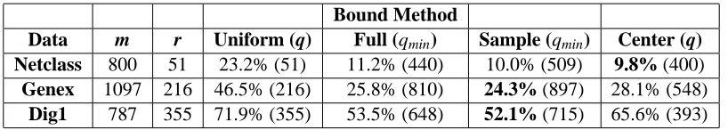
For all tests, δ = 0.01, and bounds are produced by applying Theorem 7. Each table in this section shows error bounds produced by various methods for a set of problems. For each problem, the best error bound is shown in bold. In parentheses after the bounds are values of q that produced the bounds. For methods Full and Sample, qminis the value of q∈W that minimizesε(m, r, q,δ/w)
in Theorem 7. For the other methods, the value of q shown is the only choice.
8.1 Error Bounds for SVMs Trained on Real-World Data Sets
This subsection applies the bound methods to actual data sets for which SVMs have been developed:
1. Netclass – SVMs were trained to recognize which of several generative graph models best describe a graph of the neural network of c. elegans (Middendorf et al., 2004). There are m = 800 training examples and r = 51 support vectors.
Bound Method
Data m r Uniform (q) Full (qmin) Sample (qmin) Center (q)
Netclass 800 51 23.2% (51) 11.2% (440) 10.0% (509) 9.8% (400) Genex 1097 216 46.5% (216) 25.8% (810) 24.3% (897) 28.1% (548)
Dig1 787 355 71.9% (355) 53.5% (648) 52.1% (715) 65.6% (393)
Table 1: Error Bounds for Real-World Data Sets
Bound Method
r Uniform (q) Full (qmin) Sample (qmin) Center (q)
5 25.0% (5) 19.7% (21) 17.1% (27) 15.0% (50) 10 35.6% (10) 27.2% (33) 24.5% (36) 21.3% (50) 20 50.9% (20) 39.8% (50) 36.9% (54) 34.1% (50)
Table 2: Error Bounds for m = 100 Examples
3. Dig1 – An SVM was trained for digit recognition (Langford 2005). There are m = 787 training examples and r = 355 support vectors.
Method Center produces the best bound for problem Netclass, and method Sample produces the best bound for the other problems. For the first two problems (Netclass and Genex), all methods based on nearly uniform bounds produce about the same bounds, and they are about half the error bound produced by uniform validation. For Dig1, the bounds produced by methods Full and Sample are much better than those produced by uniform validation, but still not good enough to be of any use in practice.
Why are compression bounds for Dig1 so ineffective? Compression bounds are based on the idea that if a classifier is based on only a few training examples and still performs well on the rest, then that is evidence that the classifier performs well in general. For Dig1, the size of the retained set, r, is about half of the number of training examples m. The retained set is composed of training examples used in the classifier and of training examples for which the classifier errs. Consider the following scenario: each class label is equally likely, and we simply choose g* to be the function that returns the most common label in the training set regardless of the input. Then the retained set consists of all training examples with the least common label, which is most likely a little less than half the training examples. In this case, the true error rate is 50%, and r is about half of m. Since our compression bounds are based on r and m, the bounds cannot distinguish this scenario from the case of Dig1. Hence, compression bounds rely heavily on having few retained examples relative to the number of training examples.
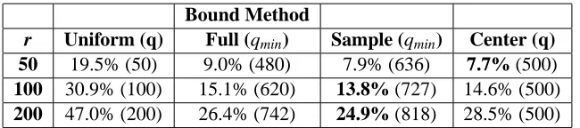
8.2 Error Bounds for m = 1000 Examples
This section explores error bounds produced by the different methods over a range of training set sizes m and retained set sizes r. These tests give a sense of how data set sizes and ratios of r to m affect bounds.
Bound Method
r Uniform (q) Full (qmin) Sample (qmin) Center (q)
50 19.5% (50) 9.0% (480) 7.9% (636) 7.7% (500) 100 30.9% (100) 15.1% (620) 13.8% (727) 14.6% (500) 200 47.0% (200) 26.4% (742) 24.9% (818) 28.5% (500)
Table 3: Error Bounds for m = 1000 Examples
Bound Method
r Uniform (q) Full (qmin) Sample (qmin) Center (q)
50 11.7% (50) 4.6% (895) 4.0% (1090) 3.9% (1000) 100 19.2% (100) 7.7% (1209) 7.0% (1454) 7.3% (1000) 200 30.6% (200) 13.6% (1374) 12.7% (1454) 14.2% (1000)
Table 4: Error Bounds for m = 2000 Examples
the bounds for the uniform method when the ratio r:m is about 1:10. The advantage of using nearly uniform methods is more pronounced for smaller ratios of r:m.
Comparing Table 2 to Table 3 cell-by-cell shows the effect of increasing problem size by a factor of 10 while keeping ratios r:m the same. In general, the bounds improve as problem size increases, and the improvement is greater for smaller r:m ratios. The same kind of comparison is possible between Table 3 and Table 4 by comparing the first two rows of Table 3 to the last two rows of Table 4. This comparison shows the same general trends.
9. Discussion
This section outlines several possible directions for future work. One possibility is to improve the bounds by treating training examples for which g* errs differently from training examples that comprise g*. Right now, these examples are combined in the retained set R. Let RE be the set of
training errors for g*, and let R* be the set of examples used to form g*. Suppose training on any superset of R* yields g*, that is, including some training errors from RE does not disrupt training.
Then R* can be used in place of R to form a new error bound on g*. Of course, we need to use validation of non-consistent classifiers in the proposed bound, since validation sets would contain examples that cause empirical error. For example, we could use the bounds based on Binomial Tail Inversion (Langford, 2005).
It would be useful to extend the results of this paper to other classifiers that have compression-based bounds, including set covering machines (SCMs) (Marchand and Shawe-Taylor 2001) and decision list machines (DLMs) (Marchand and Sokolova 2005). The challenge is to efficiently identify a retained set under the present training methods for SCMs and DLMs, that is, identify a small subset of training examples such that training on any superset that is a subset of the training examples produces the same classifier. A solution may be to modify the training algorithms in some way to make it easy to identify a small retained set after training.
An alternative approach is to empirically estimate the fraction of trainings on subsets of training data (and perhaps on strings of side information) that produce the same classifier as the classifier g* trained on all available data. Use sampling over subsets of training data (and strings of side information) to estimate the fraction. Then form an error bound that uses the estimated fraction as the basis for nearly uniform validation. Include a term in the error bound to account for the possibility of over-estimating the fraction of trainings that produce g*.
Finally, it should be possible to apply this empirical approach to nearly uniform validation in a transductive setting, where the inputs of examples to be classified are known. Each classifier g that agrees with g* on all examples to be classified could be considered equivalent to g*. This procedure is similar to empirically determining VC dimension for specific data sets, as described by Vapnik (1998).
Acknowledgments
Thanks to John Langford for extremely helpful advice, encouragement, and data. Thanks to Mario Marchand for encouragement, pointers to relevant literature, and feedback on presentation. Thanks to Manfred Warmuth and three anonymous referees for many helpful suggestions. Thanks to Lance Williams and Dan Ruderman for discussions that led to this paper and for feedback on several versions of the results. Thanks to Danny Hillis and everyone at Applied Minds for encouragement and support to pursue this research.
References
E. Bax. Similar classifiers and vc error bounds, caltechcstr:1997.cs-tr-97-14. Technical report, California Institute of Technology, 1997. Also available as
http://resolver.caltech.edu/CaltechCSTR:1997.cs-tr-97-14.
M. Brown, W. Grundy, D. Lin, N. Cristianini, C. Sugnet, M. Ares Jr., and D. Haussler. Support vec-tor machine classification of microarray gene expression data, ucsc-crl 99-09. Technical report, University California Santa Cruz, 1999.
N. Cristianini and J. Shawe-Taylor. An Introduction to Support Vector Machines and Other Kernel-Based Learning Methods. Cambridge University Press, 2000.
W. Feller. An Introduction to Probability Theory and Its Applications. John Wiley & Sons, New York, 1968.
J. Langford. Tutorial on practical prediction theory for classification. Journal of Machine Learning Research, 6:273–306, 2005.
N. Littlestone and M. Warmuth. Relating data compression and learnability, 1986. Unpublished manuscript, University of California Santa Cruz.
M. Marchand and J. Shawe-Taylor. Learning with the set covering machine. In Proceedings of the Eighteenth International Conference on Machine Learning (ICML 2001), pages 345–352, 2001.
M. Marchand and M. Sokolova. Learning with decision lists of data-dependent features. Journal of Machine Learning Research, 6:427–451, 2005.
M. Middendorf, E. Ziv, C. Adams, J. Hom, R. Koytcheff, C. Levovitz, G. Woods, L. Chen, and C. Wiggins. Discriminative topological features reveal biological network mechanisms. BMC Bioinformatics, 5(181), 2004.
V. Vapnik. Statistical Learning Theory. John Wiley & Sons, 1998.