Online Learning of Multiple Tasks with a Shared Loss

Online Learning of Multiple Tasks with a Shared Loss

Ofer Dekel [email protected]

School of Computer Science and Engineering The Hebrew University

Jerusalem, 91904, Israel

Philip M. Long [email protected]

Yoram Singer [email protected]

Google Inc.

1600 Amphitheater Parkway Mountain View, CA 94043, USA

Editor: Peter Bartlett

Abstract

We study the problem of learning multiple tasks in parallel within the online learning framework. On each online round, the algorithm receives an instance for each of the parallel tasks and responds by predicting the label of each instance. We consider the case where the predictions made on each round all contribute toward a common goal. The relationship between the various tasks is defined by a global loss function, which evaluates the overall quality of the multiple predictions made on each round. Specifically, each individual prediction is associated with its own loss value, and then these multiple loss values are combined into a single number using the global loss function. We focus on the case where the global loss function belongs to the family of absolute norms, and present several online learning algorithms for the induced problem. We prove worst-case relative loss bounds for all of our algorithms, and demonstrate the effectiveness of our approach on a large-scale multiclass-multilabel text categorization problem.

Keywords: online learning, multitask learning, multiclass multilabel classiifcation, perceptron

1. Introduction

Multitask learning is the problem of learning several related problems in parallel. In this paper, we discuss the multitask learning problem in the online learning context, and focus on the possibility that the learning tasks contribute toward a common goal. Our hope is that we can benefit from learning the tasks jointly, as opposed to learning each task independently.

loss values into a single number, and define the global loss attained on round t to be

L

(`t). At the end of this online round, the algorithm may use the k new labeled examples it has obtained to improve its prediction mechanism for the rounds to come. The goal of the learning algorithm is to suffer the smallest possible cumulative loss over the course of T rounds,∑T_t=1

L

(`t).

The choice of the global loss function captures the overall consequences of the individual pre-diction errors, and therefore how the algorithm should prioritize correcting errors. For example, if

L

(`t) is defined to be ∑kj=1`t,j then the online algorithm is penalized equally for errors on each of the tasks; this results in effectively treating the tasks independently. On the other hand, if

L

(`t) =maxj`t,j then the algorithm is only interested in the worst mistake made on each round. We do not assume that the data sets of the various tasks are similar or otherwise related. Moreover, the examples presented to the algorithm for each of the tasks may come from completely different domains and may possess different characteristics. The multiple tasks are tied together by the way we define the objective of our algorithm.

In this paper, we focus on the case where the global loss function is an absolute norm. A norm

k · kis a function such that_kv_k>0 for all v₆=0,_k0_k=0,_kλv_k=_|λ_|kv_kfor all v and allλ_∈R, and which satisfies the triangle inequality. A norm is said to be absolute if_kv_k=_k|v_|kfor all v, where

|v_|is obtained by replacing each component of v with its absolute value. The most well-known family of absolute norms is the family of p-norms (also called Lpnorms), defined for all p≥1 by

kv_kp =

n

∑

j=1

|vj|p

1/p _.

A special member of this family is the L∞norm, which is defined to be the limit of the above when p tends to infinity, and can be shown to equal maxj|vj|. A less known family of absolute norms is the family of r-max norms. For any integer r between 1 and k, the r-max norm of v_∈Rkis the sum of the absolute values of the r absolutely largest components of v. Formally, the r-max norm is

kv_kr-max = r

∑

j=1

|v_π(j)| where |vπ(1)| ≥ |vπ(2)| ≥ . . . ≥ |vπ(k)| . (1)

Note that both the L1 norm and L∞ norm are special cases of the r-max norm, as well as being

p-norms. Actually, the r-max norm can be viewed as a smooth interpolation between the L1norm and the L∞norm, using Peetre’s K-method of norm interpolation (see Appendix A for details).

Since the global loss functions we consider in this paper are norms, the global loss equals zero only if `t is itself the zero vector. Furthermore, decreasing any individual loss can only decrease the global loss function. Therefore, the simplest solution to our multitask problem is to learn each task individually, and minimize the global loss function implicitly. The natural question which is at the heart of this paper is whether we can do better than this. Our answer to this question is based on the following fundamental view of online learning. On every round, the online learning algo-rithm balances a trade-off between retaining the information it has acquired on previous rounds and modifying its hypothesis based on the new examples obtained on that round. Instead of balancing this trade-off individually for each of the learning tasks, we can balance it jointly, for all of the tasks. By doing so, we allow ourselves to make a big modification to one of the k hypotheses at the expense of the others. This additional flexibility enables us to directly minimize the specific global loss function we have chosen to use.

Multiclass Classification using the L∞Norm Assume that we are faced with a multiclass classi-fication problem, where the size of the label set is k. One way of solving this problem is by learning k binary classifiers, where each classifier is trained to distinguish between one of the classes and the rest of the classes. This approach is often called the one-vs-rest method. If all of the binary classifiers make correct predictions, then one of these predictions should be positive and the rest should be negative. If this is the case, we can correctly predict the corresponding multiclass label. However, if one or more of the binary classifiers makes an incorrect prediction, we can no longer guarantee the correctness of our multiclass prediction. In this sense, a single binary mistake on round t is as bad as many binary mistakes on round t. Therefore, we should only care about the worst binary prediction on round t, and we can do so by choosing the global loss to be_k`tk∞.

Another example where the L_∞ norm comes in handy is the case where we are faced with a

multiclass problem where the number of labels is huge. Specifically, we would like the running time and the space complexity of our algorithm to scale logarithmically with the number of labels. Assume that the number of different labels is 2k, enumerate these labels from 0 to 2k₋1, and consider the k-bit binary representation of each label. We can solve the multiclass problem by training k binary classifiers, one for each bit in the binary representation of the label index. If all k classifiers make correct predictions, then we have obtained the binary representation of the correct multiclass label. As before, a single binary mistake is devastating to the multiclass classifier, and the L_∞norm is the most appropriate means of combining the k individual losses into a global loss.

Vector-Valued Regression using the L2Norm Let us deviate momentarily from the binary clas-sification setting, and assume that we are faced with multiple regression problems. Specifically, assume that our task is to predict the three-dimensional position of an object. Each of the three co-ordinates is predicted using an individual regressor, and the regression loss for each task is simply the absolute difference between the true and the predicted value on the respective axis. In this case, the most appropriate choice of the global loss function is the L2norm, which reduces the vector of individual losses to the Euclidean distance between the true and predicted 3-D targets. (Note that we take the actual Euclidean distance and not the squared Euclidean distance often minimized in regression settings).

Error Correcting Output Codes and the r-max Norm Error Correcting Output Codes (ECOC) is a technique for reducing a multiclass classification problem to multiple binary classification prob-lems (Dietterich and Bakiri, 1995). The power of this technique lies in the fact that a correct mul-ticlass prediction can be made even when a few of the binary predictions are wrong. The reduction is represented by a code matrix M_{∈ {−}1,+1_}s×k, where s is the number of multiclass labels and k is the number of binary problems used to encode the original multiclass problem. Each row in M represents one of the s multiclass labels, and each column induces one of the k binary classification problems. Given a multiclass training set_{(xi,yi)_}m

i=1, with labels yi∈ {1, . . . ,s}, the binary prob-lem induced by column j is to distinguish between the positive examples_{(xi,yi: Myi,j= +1}and

negative examples{(xi,yi: Myi,j =−1}. When a new instance is observed, applying the k binary

classifiers to it gives a vector of binary predictions, ˆy= (y1ˆ , . . . ,ykˆ )_{∈ {−}1,+1_}k. We then predict the multiclass label of this instance to be the index of the row in M which is closest to ˆy in Hamming distance.

words, making d(M)/2 binary mistakes is as bad as making more binary mistakes. Let r=d(M)/2. If the binary classifiers are trained in the online multitask setting, we should only be interested in whether the r’th largest loss is less than 1, which would imply that a correct multiclass prediction can be guaranteed. Regretfully, taking the r’th largest element of a vector (in absolute value) does not constitute a norm and thus does not fit in our setting. However, the r-max norm, defined in Equation (1), can serve as a good proxy.

In this paper, we present three families of online multitask algorithms. Each family includes algorithms for every absolute norm. All of the algorithms presented in this paper follow the gen-eral skeleton outlined in Figure 1. Specifically, all of our algorithms use linear threshold functions as hypotheses and an additive update rule. The first two families are multitask extensions of the Perceptron algorithm (Rosenblatt, 1958; Novikoff, 1962), while the third family is closely related to the Passive-Aggressive classification algorithm (Crammer et al., 2006). Incidentally, all of the algorithms presented in this paper can be easily transformed into kernel methods. For each algo-rithm, we prove a relative loss bound, namely, we show that the cumulative global loss attained by the algorithm is comparable to the cumulative loss attained by any fixed set of k linear hypotheses, even defined in hindsight.

Much previous work on theoretical and applied multitask learning has focused on how to take advantage of similarities between the various tasks (Caruana, 1997; Heskes, 1998; Evgeniou et al., 2005; Baxter, 2000; Ben-David and Schuller, 2003; Tsochantaridis et al., 2004); in contrast, we do not assume that the tasks are in any way related. Instead, we consider how to take account of shared consequences of errors. Kivinen and Warmuth (2001) generalized the notion of matching loss (Helmbold et al., 1999) to multi-dimensional outputs. Their construction enables analysis of algorithms that perform multi-dimensional regression by composing linear functions with a variety of transfer functions. It is not obvious how to directly use their work to address the problems that fall into our setting. An analysis of the L_∞norm of prediction errors is implicit in some past work of Crammer and Singer (2001, 2003). The algorithms presented in Crammer and Singer (2001, 2003) were devised for multiclass categorization with multiple predictors (one per class) and a single instance. The present paper extends the multiclass prediction setting to a broader framework, and tightens the analysis. In contrast to the multiclass prediction setting, the prediction tasks in our setting are tied solely through a globally shared loss. When k, the number of multiple tasks, is set to 1, two of the algorithms presented in this paper as well as the multiclass algorithms in Crammer and Singer (2001, 2003) reduce to the PA-I algorithm, presented in Crammer et al. (2006). Last, we would like to mention in passing that a few learning algorithms for ranking problems decompose the ranking problem into a preference learning task over pairs of instances (see for instance Herbrich et al., 2000; Chapelle and Harchaoui, 2005). The ranking losses employed by such algorithms are typically defined as the sum over pair-based losses. Our setting generalizes such approaches for ranking learning by employing a shared loss which is defined through a norm over the individual pair-based losses.

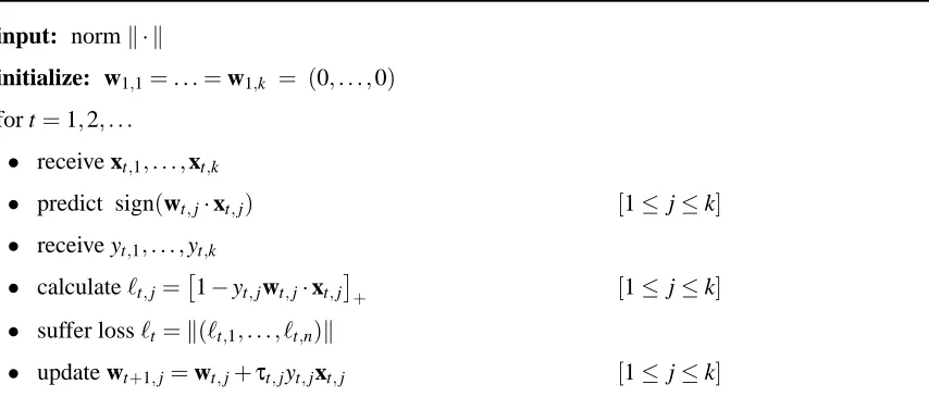
input: norm_{k · k}

initialize: w1,1=. . .=w1,k = (0, . . . ,0) for t=1,2, . . .

• receive xt,1, . . . ,xt,k

• predict sign(wt,j·xt,j) [1≤ j≤k]

• receive yt,1, . . . ,yt,k

• calculate`t,j=

1₋yt,jwt,j·xt,j

+ [1≤ j≤k]

• suffer loss`t=k(`t,1, . . . , `t,n)k

• update wt+1,j=wt,j+τt,jyt,jxt,j [1≤ j≤k]

Figure 1: A general skeleton for an online multitask classification algorithm. A concrete algorithm is obtained by specifying the values ofτt,j.

efficient algorithms for solving the implicit update in the case where the global loss is defined by the L2norm or the r-max norm. Experimental results are provided in Section 8 and we conclude the paper in Section 9 with a short discussion.

2. Online Multitask Learning with Additive Updates

We begin by presenting the online multitask classification setting more formally. We are presented with k online binary classification problems in parallel. The instances of each task are drawn from separate instance domains, and for concreteness we assume that the instances of task j are all vectors inRnj_{. As stated in the previous section, online learning is performed in a sequence of rounds.}

On round t, the algorithm observes k instances, (xt,1, . . . ,xt,k)∈Rn1×. . .×Rnk. The algorithm maintains k separate classifiers in its internal memory, one for each of the multiple tasks, which are updated from round to round. Each of these classifiers is a margin-based linear predictor, defined by a weight vector. We denote the weight vector used on round t to define the j’th predictor by wt,j and note that wt,j∈Rnj. The algorithm uses its classifiers to make k binary predictions, ˆyt,1, . . . ,ytˆ,k,

where ˆyt,j =sign(wt,j·xt,j). After making these predictions, the correct labels of the respective tasks, yt,1, . . . ,yt,k, are revealed and each one of the predictions is evaluated. In this paper we focus on the hinge-loss function as the means of penalizing incorrect predictions. Formally, the loss associated with the j’th task is defined to be

`t,j =

1₋yt,jwt,j·xt,j

+ ,

where [a]+=max{0,a}. As previously stated, the global loss is then defined to bek`tk, where

denoteτt= (τt,1, . . . ,τt,k). The general skeleton followed by all of our online algorithms is given in Figure 1.

A concept of key importance in this paper is the notion of dual norms (Horn and Johnson, 1985). Any normk · kdefined onRn_{, has a dual norm, also defined onR}n_{, denoted byk · k}∗_{and given by}

ku_k∗ = max

v∈Rn

u_·v

kv_k = v∈Rmaxn_:kvk=1u·v . (2)

The dual of a p-norm is itself a p-norm, and specifically, the dual of_{k · k}pisk · kq, where1_q+1_p =1. The dual of_{k · k∞}is_{k · k}1and vice versa. In Appendix A we prove that the dual ofkvkr-maxis

ku_k∗_r-max = max

ku_k∞,kuk1

r

. (3)

An important property of dual norms, which is an immediate consequence of Equation (2), is that for any u,v_∈Rnit holds that

u_·v _{≤ k}u_k∗_kv_k . (4)

If_{k · k}is a p-norm then the above is known as H ¨older’s inequality, and specifically, if p=2 it is called the Cauchy-Schwartz inequality. Two additional properties which we rely on are that the dual of the dual norm is the original norm (see for instance Horn and Johnson, 1985), and that the dual of an absolute norm is also an absolute norm. As previously mentioned, to obtain concrete online algorithms, all that remains is to define the update weightsτt,j for each task on each round. The different ways of settingτt,j discussed in this paper all share the following properties:

• boundedness: _∀1_≤t_≤T _kτtk∗≤C for some predefined parameter C

• non-negativity: ∀1≤t≤T,1≤ j≤k τt,j≥0

• conservativeness: _∀1_≤t_≤T,1_≤ j_≤k (`t,j=0) ⇒ (τt,j=0)

Even before specifying the exact value ofτt,j, we can state and prove a powerful lemma which is the crux of our analysis. This lemma will motivate and justify our specific choices ofτt,jthroughout this paper.

Lemma 1 Let_{(xt,j,yt,j)}1₁≤_≤tj_≤≤_Tk be a sequence of T k-tuples of examples, where each xt,j∈Rnj, and each yt,j∈ {−1,+1}. Let w1?, . . . ,w?kbe arbitrary vectors where w?j∈Rnj, and define the hinge loss attained by w?_j on example(xt,j,yt,j)to be`?t,j=

1−yt,jw?j·xt,j

+. Letk · kbe an arbitrary

norm and let_{k · k}∗ denote its dual. Assume we apply an algorithm of the form outlined in Figure 1 to this sequence of examples, where the update weights satisfy the boundedness, non-negativity and conservativeness requirements. Then, for any C>0 it holds that

T

∑

t=1

k

∑

j=1

2τt,j`t,j−τ2t,jkxt,jk22

≤

k

∑

j=1

kw?_jk2₂ + 2C T

∑

t=1

k`?tk .

Under the assumptions of this lemma, our algorithm competes with a set of fixed linear classifiers,

w?₁, . . . ,w?_k, which may even be defined in hindsight, after observing all of the inputs and their labels.

which is proportional to the cumulative loss of our competitor,∑_tT₌₁k`?

tk. The left hand side of the bound is the term

T

∑

t=1

k

∑

j=1

2τt,j`t,j−τ2t,jkxt,jk22

. (5)

This term plays a key role in the derivation of all three families of algorithms presented in the sequel. Each choice of the update weightsτt,jenables us to prove a different lower bound on Equation (5). Comparing this lower bound with the upper bound in Lemma 1 gives us a loss bound for the respec-tive algorithm. The proof of Lemma 1 is given below.

Proof Define∆t,j=kwt,j−w?jk22−kwt+1,j−w?jk22. We prove the lemma by bounding∑ T

t=1∑kj=1∆t,j

from above and from below. Beginning with the upper bound, we note that for each 1_≤ j_≤k,

∑T

t=1∆t,j is a telescopic sum which collapses to T

∑

t=1

∆t,j = kw1,j−w?k22− kwT+1,j−w?k22 .

Using the facts that w1,j= (0, . . . ,0)andkwT+1,j−w?k2₂≥0 for all 1≤ j≤k, we conclude that T

∑

t=1

k

∑

j=1

∆t,j ≤ k

∑

j=1

kw?_jk2₂ . (6)

Turning to the lower bound, we note that we can consider only non-zero summands which actually contribute to the sum, namely∆t,j6=0. Plugging the definition of wt+1,j into∆t,j, we get

∆t,j = kwt,j−w?jk22− kwt,j+τt,jyt,jxt,j−w?jk22 = τt,j −2yt,jwt,j·xt,j−τt,jkxt,jk22+2yt,jw?j·xt,j

= τt,j 2(1−yt,jwt,j·xt,j)−τt,jkxt,jk22−2(1−yt,jw?j·xt,j)

. (7)

Since our update is conservative,∆t,j6=0 implies that`t,j=1−yt,jwt,j·xt,j. By definition, it also holds that`?

t,j≥1−yt,jw?j·xt,j. Plugging these two facts into Equation (7) and using the fact that

τt,j is non-negative gives

∆t,j ≥ τt,j 2`t,j−τt,jkxt,jk22−2`?t,j

.

Summing the above over 1_≤ j_≤k gives

k

∑

j=1

∆t,j ≥ k

∑

j=1

2τt,j`t,j−τ2t,jkxt,jk22

−2

k

∑

j=1

τt,j`t?,j . (8)

Using Equation (4) we know that∑k_j=1τt,j`?t,j≤ kτtk∗k`?tk. From our assumption thatkτtk∗≤C, we have that∑k_j=1τt,j`?t,j≤Ck`?tk. Plugging this inequality into Equation (8) gives

k

∑

j=1

∆t,j ≥ k

∑

j=1

2τt,j`t,j−τ2t,jkxt,jk22

−2C_k`?tk .

3. The Finite-Horizon Multitask Perceptron

In this section, we present our first family of online multitask classification algorithms, and prove a relative loss bound for the members of this family. This family includes algorithms for any global loss function defined through an absolute norm. These algorithms are finite-horizon online algo-rithms, meaning that the number of online rounds, T , is known in advance and is given as a param-eter to the algorithm. An analogous family of infinite-horizon algorithms is the topic of the next section.

As previously noted, the Finite-Horizon Multitask Perceptron follows the general skeleton out-lined in Figure 1. Given an absolute norm_{k · k}and its dual_{k · k}∗, the multitask Perceptron setsτt,j in Figure 1 to

τt = argmax

τ:kτk∗_≤C

τ·`t , (9)

where C>0 is a constant which is specified later in this section. There may exist multiple solutions to the maximization problem above and at least one of these solutions induces a conservative update. In other words, we may assume that the solution to Equation (9) is such that τt,j =0 at every coordinate j where`t,j =0. To see that such a solution exists, take an arbitrary optimal solutionτ and let ˆτbe defined by

ˆ

τj =

_τ

j if`t,j6=0 0 if`t,j=0.

Clearly, τ_·`t =ˆτ·`t, whereaskˆτk∗≤ kτk∗≤C. If the optimization problem in Equation (9) has multiple solutions that induce conservative updates, assume that one is chosen arbitrarily.

An equivalent way of defining the solution to Equation (9) is by satisfying the equalityτt·`t= C<sub>k</sub>`tk. To see this equivalence, note that the dual ofk · k∗is defined by Equation (2) to be

k`_k∗∗ = max

τ:_kτ_k∗_≤1τ·` .

However, since_{k · k}∗∗ is equivalent to_{k · k}(see for instance Theorem 5.5.14 in Horn and Johnson, 1985), we get

k`_k = max

τ:kτk∗_≤1 τ·` .

Using the linearity of_{k · k}∗, we conclude that_kτ/C_k∗ =_kτ_k∗/C for any C>0, and therefore the above becomes

C_k`_k = max

τ:_kτ_k∗_≤C τ·` .

We conclude that

τt·`t = Ck`tk (10)

holds if and only ifτt is a maximizer of Equation (9).

When the global loss function is a p-norm, the following definition ofτt solves Equation (9):

τt,j =

C`<sub>t</sub>p<sub>,</sub>−<sub>j</sub> 1 k`tkpp−1

. (11)

When the global loss function is an r-max norm andπis a permutation such that`t,π(1)≥. . .≥`t,π(k),

the following definition ofτt is a solution to Equation (9):

τt,j =

C if `t,j>0 and j∈ {π(1), . . . ,π(r)}

1 1 6

√

2 √2

L1norm L2norm L3norm L_∞norm

Figure 2: The remoteness of a norm is the longest Euclidean length of any vector contained in the norm’s unit ball. The longest vector in each of the two-dimensional unit balls above is depicted with an arrow.

Note that when r=k, the r-max norm reduces to the L1norm and the above becomes the well-known update rule of the Perceptron algorithm (Rosenblatt, 1958; Novikoff, 1962). The correctness of the definitions in Equation (11) and Equation (12) can be easily verified by observing that _kτtk∗≤C and thatτt·`t=Ck`tkin both cases.

Before proving a loss bound for the multitask Perceptron, we must introduce another important quantity. This quantity is the remoteness of a norm_{k · k}defined onRk, and is defined to be

ρ(_{k · k},k) = max

u∈Rk

ku_k2

ku_k = u∈Rmaxk_:kuk≤1kuk2 . (13)

Geometrically, the remoteness of_{k · k}is simply the Euclidean length of the longest vector (again, in the Euclidean sense) which is contained in the unit ball of_{k · k}. This definition is visually depicted in Figure 2. As we show below, the remoteness of the dual norm, ρ(_{k · k}∗_{,k), plays an important} role in determining the difficulty of using_{k · k}as the global loss function.

For concreteness, we now calculate the remoteness of the duals of p-norms and of r-max norms.

Lemma 2 The remoteness of a p-norm_{k · k}qequals

ρ(_{k · k}q,k) =

(

1 if 1_≤q_≤2

k(12− 1

q) _{if 2}<_q .

Before proving the lemma, we note that if _{k · k}p is a p-norm and k · kq is its dual, then we can combine Lemma 2 with the equality q= _p−p₁ to obtain

ρ(_{k · k}q,k) =

(

1 if 2_≤p

k(1p−

1

2) _{if 1}≤_p<₂ .

This equivalent form is better suited to our needs. The proof of Lemma 2 is given below.

setting v= (1,0, . . . ,0), we getkvkq=kvk2and thereforeρ(k · kq,k)≥1. Overall, we have shown thatρ(_{k · k}q,k) =1.

Turning to the case where 1_≤p<2, we note that q>2. Let v be an arbitrary vector inRk, and define u= (v2₁, . . . ,v2_k)and w= (1, . . . ,1). Noting thatk · kq

2 andk · k

q

q−2 are dual norms, we use H¨older’s inequality to obtain

u_·w _{≤ k}u_kq

2kwk

q q−2 .

The left-hand side above equals_kv_k2₂, while the right-hand side above equals _kv_k2_qk1−2q_.

There-fore, _kv_k2₂/_kv_kq2_≤k1−2q _{and taking square-roots on both sides yields}k_vk

2/kvkq≤k 1 2−

1

q_{. Since}

this inequality holds for all v_∈Rk, we have shown that ρ(_{k · k}q,k)≤k 1 2−

1

q_{. On the other hand,}

setting v= (1, . . . ,1), we get_kv_k2=k 1 2−

1

q_{kvkq. This proves that}ρ_{(k · k}

q,k)≥k 1 2−

1

q_{, and therefore}

ρ(_{k · k}q,k) =k 1 2−

1

q_.

Lemma 3 Let_{k · k}r-max be a r-max norm and letk · k∗r-max be its dual. The remoteness ofk · k∗r-max equals√r.

Proof Using Equation (13), the remoteness of_{k · k}∗_r-maxis defined to be the maximum value of_ku_k2 subject to _ku_k∗_{r-max ≤}1. Recalling the definition of _{k · k}∗_r-max from Equation (3), we can replace this constraint with two constraints_ku_k1≤r andkuk∞≤1. Moreover, since both the L1norm and the L∞ norm are absolute norms, we can also assume that u resides in the non-negative orthant. Therefore, we have that 0_≤uj≤1 for all 1≤ j≤k. From this we conclude that u2j ≤uj for all 1_≤ j_≤k, and thus_ku_k2_{2≤ k}u_k1≤r. Hence, kuk2≤√r andρ(k · k∗r-max,k)≤

√

r. On the other hand, the vector

u = r

z }| {

1, . . . ,1,

k₋r

z }| {

0, . . . ,0

is contained in the unit ball of_{k · k}∗_r-max, and its Euclidean length is√r. Therefore, we also have that

ρ(_{k · k}∗_r-max,k)_≥√r, and overall we getρ(_{k · k}∗_r-max,k) =√r.

We are now ready to prove a loss bound for the Finite-Horizon Multitask Perceptron.

Theorem 4 Let_{(xt,j,yt,j)}11≤≤tj≤≤Tk be a sequence of T k-tuples of examples, where each xt,j∈Rnj,

kxt,jk2≤R and each yt,j∈ {−1,+1}. Let C be a positive constant and letk·kbe an absolute norm. Let w?₁, . . . ,w?_k be arbitrary vectors where w?_{j ∈}Rnj_{, and define the hinge loss incurred by w}?

j on example(xt,j,yt,j)to be`?t,j =

1₋yt,jw?j·xt,j

+. If we present this sequence to the finite-horizon

multitask Perceptron with the norm_{k · k}and the aggressiveness parameter C, then,

T

∑

t=1

k`tk ≤ 1 2C

k

∑

j=1

kw?_jk2₂ + T

∑

t=1

k`?tk +

T R2Cρ2(_{k · k}∗,k)

2 .

of the lemma, and we have

T

∑

t=1

k

∑

j=1

2τt,j`t,j−τ2t,jkxt,jk22

≤

k

∑

j=1

kw?_jk2₂ + 2C T

∑

t=1

k`?tk .

Using Equation (10), we rewrite the left-hand side of the above as

2C T

∑

t=1

k`tk − T

∑

t=1

k

∑

j=1

τ2

t,jkxt,jk22 . (14) Using our assumption that _kxt,jk22 ≤R2, we know that ∑kj=1τt2,jkxt,jk22 ≤(Rkτtk2)2. Using the definition of remoteness, we can upper bound this term by(R_kτtk∗ρ(k · k∗,k))2. Finally, using our upper bound on_kτtk∗we can further bound this term by R2C2ρ2(k · k∗,k). Plugging this bound back into Equation (14) gives

2C T

∑

t=1

k`tk − T R2C2ρ2(k · k∗,k) . Overall, we have shown that

2C T

∑

t=1

k`tk − T R2C2ρ2(k · k∗,k) ≤ k

∑

j=1

kw?_jk2₂ + 2C T

∑

t=1

k`?tk .

Dividing both sides of the above by 2C and rearranging terms gives the desired bound.

In its current form, the bound in Theorem 4 may seem insignificant, since its right-most term grows linearly with the length of the input sequence, T . This term can be easily controlled by setting C to a value on the order of 1/√T .

Corollary 5 Under the assumptions of Theorem 4, if C=1/(√T R2), then T

∑

t=1

k`tk ≤ T

∑

t=1

k`?tk +

√

T

2 R

2

∑

k j=1

kw?_jk2₂ + ρ2_{(k · k}∗_,k)

!

.

This corollary bounds the global loss cumulated by our algorithm with the global loss obtained by any fixed set of hypotheses, plus a term which grows sub-linearly in T . The significance of this term depends on the magnitude of the constant

1

2 R

2

∑

k j=1

kw?_jk2₂ + ρ2(_{k · k}∗,k)

!

.

Our algorithm uses C in its update procedure, and the value of C depends on√T . Therefore, the algorithm is a finite horizon algorithm.

task independently using a separate single-task Perceptron. We show this by presenting a simple counter-example. Specifically, we construct a concrete k-task problem with a specific global loss, an arbitrarily long input sequence_{(xt,j,yt,j)}11≤≤tj≤≤Tk, and fixed weight vectors u1, . . . ,uk to use for comparison. We then prove that

k+1 2

T

∑

t=1

k`?tk∞ ≤ T

∑

t=1

k`ˆtk∞ , (15)

where ˆ`t is the vector of individual losses of the k independent single-task Perceptrons, and, as before,`?t is the vector of individual losses of u1, . . . ,uk respectively. This example demonstrates that a claim along the lines of Corollary 5 cannot be proven for the set of independent single-task Perceptrons.

First, we would like to emphasize that we are considering a version of the single-task Perceptron that updates its hypothesis whenever it suffers a positive hinge-loss, and not only when it makes a

prediction mistake. Moreover, when an update is performed, the algorithm defines wt+1=wt+

Cytxt, where C is a predefined constant. This version of the Perceptron is sometimes called the aggressive Perceptron. If we were to use the simplest version of the Perceptron, which updates its hypothesis only when a prediction mistake occurs, then finding a counter-example that achieves Equation (15) would be trivial, without even using the distinction between single-task and multitask Perceptron learning.

Also, we can assume without loss of generality that 1/C=o(T), since otherwise, even in the case k=1, simply repeating the same example over and over provides a counterexample.

Moving on to the counter-example itself, assume that our global loss is defined by the L_∞norm. Let k be at least 2, assume that the instances of all k problems are two dimensional vectors, and set u1=. . .=uk = (1,1). Each of the single-task Perceptrons initializes its hypothesis to (0,0). Assume that all of the labels in the input sequence are positive labels. For t=0, we set x1,1=. . .= x1,k= (1,0). Each one of the independent Perceptrons suffers a positive individual loss and updates its weight vector to (C,0). We continue presenting the same example for_d1/C_{e −}1 additional rounds, which is precisely when all k weight vectors of the Perceptrons become equal to(α,0), with

α≥1. For instance, if C=O(1/√T)then the vector(1,0)is presented O(√T)times. Meanwhile, the fixed weight vectors u1, . . . ,uksuffer no loss at all.

Define t0=d1/Ce, and note that the index of the next online round is t0+1. For each t in t0+1, . . . ,t0+k, we set xt,t−t0 to(0,1)and xt,jto(1,0)for all j6=t−t0. On round t, the(t−t0)’th Perceptron, whose weight vector is (α,0), suffers an individual loss of 1 and updates its weight vector to(α,C). The remaining k₋1 Perceptrons suffer no individual loss and do not modify their weight vectors. Consequently,k<sub>`</sub>ˆ<sub>tk∞=1 on each of these rounds. Once again, the fixed vectors</sub> u1, . . . ,uksuffer no loss at all. On round t=t0+k+1, we set xt,1=. . .=xt,k= (0,−1). As a result, each of the Perceptrons suffers a hinge loss of 1+C and updates its weight vector back to(α,0). Since C is positive, we get<sub>k</sub>`ˆtk∞≥1. Meanwhile,k`?tk∞=2. We now have that

t0+k+1

∑

t=t0+1

k`ˆtk∞ ≥ k+1 and

t0+k+1

∑

t=t0+1

k`?tk∞ = 2 .

This concludes the presentation of the counter-example thus showing that a set of independent single-task Perceptrons does not attain no-regret with respect to the L∞norm global loss. Similar constructions can be given for other global loss functions. The exception is the L1 norm, which naturally reduces the multitask Perceptron to k independent single-task Perceptrons.

4. An Extension to the Infinite Horizon Setting

In the previous section, we devised an algorithm which relied on prior knowledge of T , the input sequence length. In this section, we adapt the update procedure from the previous section to the infinite horizon setting, where T is not known in advance. Moreover, the bound we prove in this section holds simultaneously for every prefix of the input sequence. This generalization comes at a price; we can only prove an upper bound on ∑_tmin_{`t, `2t}, a quantity similar to the cumulative global loss, but not the global loss per se.

To motivate our inhorizon algorithm, we take a closer look at the analysis of the finite-horizon algorithm. In the proof of Theorem 4, we lower-bounded the term∑k_j=12τt,j`t,j−τ2t,jkxt,jk22 by 2C<sub>k</sub>`tk −R2C2ρ2(k · k∗,k). The first term in this lower bound is proportional to the global loss suffered on round t, and the second term is a constant. When_k`tkis smaller than this constant, our lower bound becomes negative. This suggests that the update step-size applied by the finite-horizon Perceptron may have been too large, and that the update step may have overshot its target. As a result, the new hypothesis may be inferior to the previous one. Nevertheless, over the course of T rounds, our positive progress is guaranteed to overshadow our negative progress, and thus we are able to prove Theorem 4. However, if we are interested in a bound which holds for every prefix of the input sequence, we must ensure that every individual update makes positive progress. Concretely, we derive an update for which ∑k<sub>j=1</sub>2τt,j`t,j−τt2,jkxt,jk22 is guaranteed to be non-negative. The vectorτt remains in the same direction as before, but by setting its length more carefully, we enforce an update step-size which is never excessively large.

We use ρto abbreviate ρ(_{k · k}∗,k) throughout this section. We replace the definition ofτt in Equation (9) with the following definition,

τt = argmax

τ:kτk∗_≤minn_C,k`tk

R2ρ2

oτ·`t , (16)

where C>0 is a user defined parameter and R>0 is an upper bound on_kxt,jk2for all 1≤t≤T and all 1_≤ j_≤k. As in the previous section, we assume thatτt,j =0 whenever`t,j =0. As in Equation (10), the solution to Equation (16) can be equivalently defined by the equation

τt·`t = min

C,k`tk

R2ρ2

k`tk . (17)

When the global loss function is a p-norm, the following definition ofτt solves Equation (16):

τt,j =

   

  

`_tp_,−_j1

R2ρ2_k`

tkpp−2

if _k`tkp≤R2Cρ2 C`tp,−j1

k`tkpp−1 if k`tkp>R

When the global loss function is an r-max norm andπis a permutation such that`<sub>t,π(1)≥</sub>. . .<sub>≥</sub>`_t,π(k), then the following definition ofτt is a solution to Equation (16):

τt,j =

        

k`tkr-max

rR2 if `t,j>0 and k`tkr-max≤R2Cρ2 and j∈ {π(1), . . . ,π(r)} C if `t,j>0 and k`tkr-max>R2Cρ2 and j∈ {π(1), . . . ,π(r)}

0 otherwise.

The correctness of both definitions of τt,j given above can be verified by observing that kτtk∗≤ min_{C,k`tk

R2_ρ2}and thatτt·`t =min{C,<sub>R</sub>k2`t_ρk2}k`tkin both cases. We now turn to proving an infinite-horizon cumulative loss bound for our algorithm.

Theorem 6 Let_{(xt,j,yt,j)}t1=≤1j,≤2,...k be a sequence of k-tuples of examples, where each xt,j∈Rnj,

kxt,jk2≤R and each yt,j ∈ {−1,+1}. Let C be a positive constant, letk · kbe an absolute norm, and letρbe an abbreviation for ρ(_{k · k}∗,k). Let w₁?, . . . ,w?_k be arbitrary vectors where w?_{j ∈}Rnj_,

and define the hinge loss attained by w?_j on example(xt,j,yt,j)to be`?t,j=

1₋yt,jw?j·xt,j

+. If we

present this sequence to the explicit multitask algorithm with the norm_{k · k}and the aggressiveness parameter C, then for every T

1/(R2ρ2)

∑

t≤T :k`tk≤R2Cρ2

k`tk2 +C

∑

t≤T :k`tk>R2Cρ2

k`tk ≤ 2C T

∑

t=1

k`?tk + k

∑

j=1

kw?_jk2₂ .

Proof The starting point of our analysis is again Lemma 1. The choice ofτt,j in Equation (16) is clearly bounded by_kτtk∗≤C and conservative. It is also non-negative, due to the fact thatk · k∗is absolute and that`t,j≥0. Therefore,τt,j meets the requirements of Lemma 1, and we have

T

∑

t=1

k

∑

j=1

2τt,j`t,j−τ2t,jkxt,jk22

≤

k

∑

j=1

kw?_jk2₂ + 2C T

∑

t=1

k`?tk . (18)

We now prove our theorem by lower-bounding the left hand side of Equation (18) above. We analyze two different cases. First, if_k`tk ≤R2Cρ2then min{C,k`tk/(R2ρ2)}=k`tk/(R2ρ2). Together with Equation (17), this gives

2 k

∑

j=1

τt,j`t,j = 2kτtk∗k`tk = 2k

`tk2

R2ρ2 . (19)

On the other hand,∑k_j=1τ_t2_,jkxt,jk22can be bounded bykτtk22R2. Using the definition of remoteness, we bound this term by(_kτtk∗)2R2ρ2. Using the fact that,kτtk∗≤ k`tk/(R2ρ2), we bound this term by<sub>k</sub>`tk2/(R2ρ2). Overall, we have shown that

k

∑

j=1

τ2

t,jkxt,jk22 ≤ k

`tk2 R2ρ2 .

Subtracting both sides of the above inequality from the respective sides of Equation (19) gives

k`tk2 R2ρ2 ≤

k

∑

j=1

2τt,j`t,j−τt2,jkxt,jk22

Moving on to the second case, ifk`tk>R2Cρ2then min{C,k`tk/(R2ρ2)}=C. Using Equation (17), we have that

2 k

∑

j=1

τt,j`t,j = 2kτtk∗k`tk = 2Ck`tk . (21)

As before, we can upper bound∑k_j=1τ_t2_,jkxt,jk2₂by(kτtk∗)2R2ρ2. Using the fact that,kτtk∗≤C we can bound this term by C2R2ρ2. Finally, using our assumption that_k`tk>R2Cρ2, we conclude that

k

∑

j=1

τ2

t,jkxt,jk22 < Ck`tk .

Subtracting both sides of the above inequality from the respective sides of Equation (21) gives

C_k`tk ≤ k

∑

j=1

2τt,j`t,j−τt2,jkxt,jk22

. (22)

Comparing the upper bound in Equation (18) with the lower bounds in Equation (20) and Equa-tion (22) proves the theorem.

Corollary 7 Under the assumptions of Theorem 6, if C is set to be 1/(R2ρ2)then for every T0_≤T it holds that,

T0

∑

t=1

min_k`tk2,k`tk ≤ 2 T0

∑

t=1

k`?tk + R2ρ2 k

∑

j=1

kw?_jk2₂ .

As noted at the beginning of this section, we do not obtain a cumulative loss bound per se, but rather at a bound on∑_tmin_{`t, `2t}. However, this bound holds simultaneously for every prefix of the input sequence, and the algorithm does not rely on knowledge of the input sequence length.

5. The Implicit Online Multitask Update

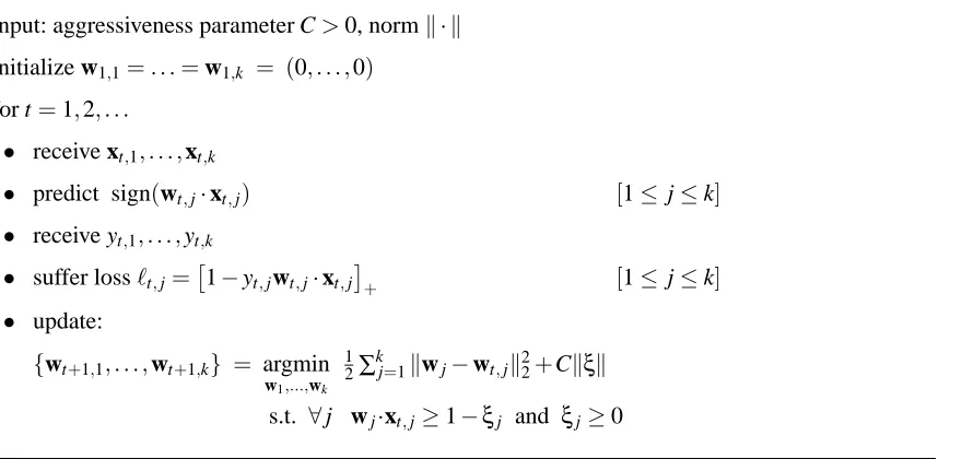
We now discuss a third family of online multitask algorithms, which leads to the strongest loss bounds of the three families of algorithms presented in this paper. In contrast to the closed form updates of the previous algorithms, the algorithms in this family require solving an optimization problem on every round, and are therefore called implicit update algorithms. Although the imple-mentation of specific members of this family may be more involved than the impleimple-mentation of the multitask Perceptron, we recommend using this family of algorithms in practice. On every round, the set of hypotheses is updated according to the update rule:

{wt+1,1, . . . ,wt+1,k} = argmin

w1,...,wk

1 2

k

∑

j=1

kwj−wt,jk22+Ckξk (23) s.t. _∀j wj·xt,j≥1−ξj and ξj≥0.

input: aggressiveness parameter C>0, norm_{k · k}

initialize w1,1=. . .=w1,k = (0, . . . ,0) for t=1,2, . . .

• receive xt,1, . . . ,xt,k

• predict sign(wt,j·xt,j) [1≤ j≤k]

• receive yt,1, . . . ,yt,k

• suffer loss`t,j=

1₋yt,jwt,j·xt,j

+ [1≤ j≤k]

• update:

{wt+1,1, . . . ,wt+1,k} = argmin

w1,...,wk

1 2∑

k

j=1kwj−wt,jk22+Ckξk s.t. _∀j wj·xt,j≥1−ξj and ξj≥0

Figure 3: The implicit update algorithm

the other hand, the term_kξ_kin the objective function, together with the constraints onξj, forces the algorithm to make progress using the new examples obtained on this round. Different choices of the global loss function lead to different definitions of this progress. The pseudo-code of the implicit update algorithm is presented in Figure 3.

Our first task is to show that this update procedure follows the skeleton outlined in Figure 1, and satisfies the requirements of Lemma 1. We do so by finding the dual of the optimization problem given in Equation (23).

Lemma 8 Let_{k · k} be a norm and let_{k · k}∗ be its dual. Then the online update defined in Equa-tion (23) is equivalent to setting wt+1,j=wt,j+τt,jyt,jxt,jfor all 1≤ j≤k, where

τt = argmax

τ

k

∑

j=1

2τj`t,j−τ2jkxt,jk22

s.t. _kτ_k∗_≤C and ∀j τj≥0 .

Moreover, this update is conservative.

Proof The update step in Equation (23) sets the vectors wt+1,1, . . . ,wt+1,k to be the solution to the following constrained minimization problem:

min

w1,...,wk,ξ≥0

1 2

k

∑

j=1

kwj−wt,jk22 +Ckξk s.t. _∀j yt,jwj·xt,j ≥ 1−ξj .

to

max

τ≥0 w1,...,minwk,ξ≥0

L

(τ,w1, . . . ,wk,ξ) ,

where

L

(τ,w1, . . . ,wk,ξ)is defined as follows:

1 2

k

∑

j=1

kwj−wt,jk22+Ckξk+ k

∑

j=1

τj(1−yt,jwj·xt,j−ξj) .

We can rewrite

L

as the sum of two terms, the first a function ofτand w1, . . . ,wk (denoted

L

1) and the second a function ofτandξ1, . . . ,ξk(denoted

L

2),

1 2

k

∑

j=1

kwj−wt,jk22+ k

∑

j=1

τj(1−yt,jwj·xt,j)

| {z }

L1(τ,w1,...,wk)

+ C_kξ_{k −} k

∑

j=1

τjξj

| {z }

L2(τ,ξ)

.

Using the notation defined above, our optimization problem becomes,

max

τ≥0

min

w1,...,wk

L

1(τ,w1, . . . ,wk) + min

ξ≥0

L

2(τ,ξ)

.

For any choice ofτ,

L

1is a convex function and we can find w1, . . . ,wkwhich minimize it by setting all of its partial derivatives with respect to the elements of w1, . . . ,wkto zero. Namely,

∀j,l 0 = ∂

L

1

∂wj,l

= wj,l−wt,j,l−τjyt,jxt,j,l .

from the above we conclude that wj=wt,j+τjyt,jxt,jfor all 1≤ j≤k.

The next step is to show that the update is conservative. If`t,j=0 then setting wj=wt,jsatisfies the constraint yt,jwj·xt,j≥1−ξj with any choice ofξj≥0. Since choosing wj =wt,j minimizes

kwt−wt,jk22and does not restrict our choice of any other variable, then it is optimal. The relation between wj andτj now implies thatτj=0 whenever`t,j=0).

Plugging our expression for wj into

L

1, we have that

min

w1,...,wk

L

1(τ,w1, . . . ,wk) = k

∑

j=1

τj(1−yt,jwt,j·xt,j) − 1 2

k

∑

j=1

τ2

jkxt,jk .

Since the update is conservative, it holds thatτj(1−yt,jwt,j·xt,j) =τj`t,j. Overall, we have reduced our optimization problem to

τt = argmax

τ≥0 k

∑

j=1

τj`t,j−

1 2τ

2 jkxt,jk

+ min

ξ≥0

L

2(τ,ξ)

!

.

We finally turn our attention to

L

2and abbreviate B(τ) =minξ_≥0

L

2(τ,ξ). We now claim that B is a barrier function for the constraint_kτ_k∗_≤C, namely

B(τ) =

0 if_kτ_k∗_≤C

To see why this is true, recall thatkτk∗_{is defined to be}

kτk∗ = max

ε∈Rk

∑k j=1τjεj

kεk .

First, let us consider the case where_kτ_k∗>C. In this case there exists a vector ¯εfor which

k

∑

j=1

τjε¯j−Ckε¯k > 0 .

Denote the left hand side of the above byδ. We can assume w.l.o.g. that all the components of ¯εare non-negative sinceτ≥0. For any c≥0, we now have that

B(τ) = min

ξ≥0

L

2(τ,ξ) ≤

L

2(τ,c¯ε) = −cδ .

Therefore, by taking c to infinity we get that B(τ) =₋∞.

Turning to the case _kτ_k∗_≤C, we have that∑k_j=1τjξj ≤Ckξkfor any choice of ξ, or in other words, min_ξ≥0

L

2(τ,ξ)≥0. However, this lower bound is attainable by settingξ=0. We conclude that if_kτ_k∗_≤C then B(τ) =0. The original optimization problem has reduced to the form

τt = argmax

τ≥0 k

∑

j=1

τj`t,j−

1 2τ

2 jkxt,jk

+ B(τ)

!

.

Clearly, the above is maximized in the domain where B(τ) =0. Therefore, we replace the function B with the constraint_kτ_k∗_≤C, and get

τt = argmax

τ≥0 :kτk∗_≤C

k

∑

j=1

τj`t,j−

1 2τ

2 jkxt,jk

.

Lemma 5 proves that the implicit update essentially finds the value ofτt that maximizes the left-hand side of the bound in Lemma 1. This choice ofτt produces the tightest loss bounds that can be derived from Lemma 1. In this sense, the implicit update algorithm takes full advantage of our proof technique. An immediate consequence of this observation is that the loss bounds of the multitask Perceptron also hold for the implicit algorithm. More precisely, the bound in Theorem 4 (and Corollary 5) holds not only for the multitask Perceptron, but also for the implicit update algorithm. Equivalently, it can be shown that the bound in Theorem 6 (and Corollary 7) also holds for the implicit update algorithm. We prove this formally below.

Theorem 9 The bound in Theorem 4 also holds for the implicit update algorithm.

Proof Letτ_t0_,j denote the weights defined by the multitask Perceptron in Equation (9) and letτt,j denote the weights assigned by the implicit update algorithm. In the proof of Theorem 4, we showed that,

2C_k`tk −R2C2ρ2 ≤ k

∑

j=1

2τ_t0_,j`t,j−τt0,2jkxt,jk22

According to Lemma 8, the weightsτt,jmaximize,

k

∑

j=1

2τt,j`t,j−τt2,jkxt,jk22

,

subject to the constraints_kτtk∗≤C andτt,j≥0. Since the weightsτt0,jalso satisfy these constraints, it holds that,

k

∑

j=1

2τ_t0_,j`t,j−τt02,jkxt,jk22

≤

k

∑

j=1

2τt,j`t,j−τ2t,jkxt,jk22

.

Therefore, we conclude that

2C_k`tk −R2C2ρ2 ≤ k

∑

j=1

2τt,j`t,j−τ2t,jkxt,jk22

. (24)

Sinceτt,j is bounded, non-negative, and conservative (due to Lemma 8), the right-hand side of the above inequality is upper-bounded by Lemma 1. Comparing the bound in Equation (24) with the bound in Lemma 1 proves the theorem.

In the remainder of this paper, we present efficient algorithms which solve the optimization problem in Equation (23) for different choices of the global loss function.

6. Solving the Implicit Update for the L2Norm

Consider the implicit update with the L2norm, namely we are trying to solve

τt = argmax

τ≥0 :kτk2≤C k

∑

j=1

τj`t,j−

1 2τ

2 jkxt,jk

.

The Lagrangian of this optimization problem is

L

=

k

∑

j=1

2τt,j`t,j−τ2t,jkxt,jk22

−θ

k

∑

j=1

τ2 t,j−C2

!

,

where θis a non-negative Lagrange multiplier. The derivative of

L

with respect to each τt,j is, 2`t,j−2τt,jkxt,jk22−2θτt,j .Setting this derivative to zero, we get

τt,j =

`t,j

kxt,jk22+θ

.

The optimum of the unconstrained problem is attained by choosing τt,j = _kx`t,j

t,jk22

for each j. If,

for this choice ofτt, the constraint ∑kj=1τ2t,j≤C2does not hold, thenθmust be greater than zero. The KKT complementarity condition implies that in this case the constraint is binding, namely

∑k

j=1τ2t,j=C2. In order to findθ, we must now solve the following equation: k

∑

j=1

`t,j

kxt,jk22+θ

2

The left hand side of the above is monotonically decreasing inθ. We also know thatθ>0. More-over, setting

θ =

√

k_k`tk∞ C

in the left-hand side of Equation (25) yields a value which is at least C2, and therefore we conclude thatθ_≤

√ kk`tk∞

C . These properties enable us to easily findθusing binary search.

In the special case where the norms of all the instances are equal, namely _kxt,1k22 =. . .=

kxt,kk22=R2, Equation (25) gives θ = k

`tk2

C −R2,and therefore τt,j =C`t,j/k`tk2. The general expression forτt,j in this case becomes

τt,j =

 

 `t,j

R2 ifk`tk2 ≤ R2C C`t,j

k`tk2 otherwise

.

Note that the above coincides with the definition ofτt given by the Infinite Horizon Multitask Per-ceptron for the L2norm, as defined in Section 4.

7. Solving the Implicit Update for r-max Norms

We now present an efficient procedure for calculating the update in Equation (23), in the case where the norm being used is the r-max norm. Lemma 8, together with (3), tells us that the update can be calculated by solving the following constrained optimization problem:

τt = argmax

τ

k

∑

j=1

2τj`t,j−τ2jkxt,jk22

(26)

s.t.

k

∑

j=1

τj≤Cr, ∀j τj≤C, ∀j τj≥0 .

After dividing the objective function by 2, the Lagrangian of this optimization problem is

k

∑

j=1

τj`t,j−

1 2τ

2 jkxt,jk22

+θCr₋ k

∑

j=1

τj

+ k

∑

j=1

λj(C−τj) + k

∑

j=1

βjτj ,

where θ, the βj’s and the λj’s are non-negative Lagrange multipliers. The derivative of

L

with respect to eachτj is,`t,j−τjkxt,jk2₂−θ−λj+βj. All of these partial derivatives must equal zero at the optimum, and therefore

∀1_≤ j_≤k τj=

`t,j−θ−λj+βj

kxt,jk22

. (27)

The KKT complementarity condition states that the following equalities hold at the optimum:

∀1_≤ j_≤k λj(C−τj) =0 and βjτj=0. (28)

1. Assume that`t,j−θ<0. Since bothτjandλjmust be non-negative, then from the definition ofτjin Equation (27) we learn thatβjmust be at leastθ−`t,j. In other words,βj is positive. Referring to the right-hand side of Equation (28), we conclude thatτj=0.

2. Assume that 0_≤`t,j−θ≤Ckxt,jk2₂. Summing the two equalities in Equation (28) and plug-ging in the definition ofτjfrom Equation (27) results in,

λj

C₋`t,j−θ

kxt,jk2₂

+βj

`t,j−θ

kxt,jk2₂

+(βj−λj) 2

kxt,jk2₂

= 0 . (29)

Using our assumption that`t,j−θ≥0, along with the requirement thatβj ≥0, gives us that

β(`t,j−θ)/kxt,jk22≥0. Equivalently, using our assumption that `t,j−θ≤Ckxt,jk22 along with the requirement thatλj ≥0 results inλ C−(`t,j+θ)/kxt,jk22

≥0. Plugging the last two inequalities back into Equation (29) gives,(βj−λj)2/kxt,jk22≤0. The only way that this inequality can hold is if(βj−λj) =0. Thus, the definition ofτj in Equation (27) reduces to

τj = _k`t_x,j−θ

t,jk22

.

3. Finally, assume that`t,j−θ>Ckxt,jk22. Sinceτj ≤ kτk∞≤C andβj≥0, then from Equa-tion (27) we conclude that λj is at least`t,j−θ−Ckxt,jk22. In other words, λj is positive. Referring to the left-hand side of Equation (28), we conclude that(C₋τj) =0, andτj=C.

Overall, we have shown that there exists someθ_≥0 such that the optimal update weights take the form

τt,j =

  

 

0 if `t,j−θ<0

`t,j−θ

kxt,jk22

if 0_≤`t,j−θ≤Ckxt,jk22 C if C<sub>k</sub>xt,jk22< `t,j−θ

. (30)

That is, if the individual loss of task j is smaller thanθthen no update is applied to the respective classifier. If the loss is moderate then the size of the update step is proportional to the loss attained, and inverse proportional to the squared norm of the respective instance. In any case, the size of the update step cannot exceed the fixed upper limit C.

We are thus left with the problem of finding the value of θin Equation (30) which yields the update weights that maximize Equation (26). We denote this value byθ?. First note that if we lift the constraint∑k_j=1τt,j ≤rC then the maximum of Equation (26) is obtained by settingτt,j= min_{`t,j/kxt,jk22,C}for all j, which is equivalent to settingθ=0 in Equation (30). Therefore, if

k

∑

j=1

min

`t,j

kxt,jk22

,C

≤ rC ,

the solution to Equation (26) isτt,j=min{`t,j/kxt,jk22,C}for all j. Thus, we can focus our attention on the case where

k

∑

j=1

min

`t,j

kxt,jk2₂

,C

> rC .

In this case,θ?must be non-zero in order for the constraint∑k_j=1τj≤rC to hold. Once again using the KKT complementarity condition, it follows that∑k_j=1τt,j=rC. Now, for every value ofθ, define the following two sets of indices: