A Simulation-Based Algorithm for Ergodic Control of Markov Chains Conditioned on Rare Events

A Simulation-Based Algorithm for Ergodic Control of Markov Chains

Conditioned on Rare Events

Shalabh Bhatnagar [email protected]

Department of Computer Science and Automation Indian Institute of Science

Bangalore 560 012, India

Vivek S. Borkar [email protected]

School of Technology and Computer Science

Tata Institute of Fundamental Research, Homi Bhabha Road Mumbai 400 005, India

Madhukar Akarapu [email protected]

Oracle India Pvt Ltd. Bangalore - 560 029, India

Editor: Shie Mannor

Abstract

We study the problem of long-run average cost control of Markov chains conditioned on a rare event. In a related recent work, a simulation based algorithm for estimating performance measures associated with a Markov chain conditioned on a rare event has been developed. We extend ideas from this work and develop an adaptive algorithm for obtaining, online, optimal control policies conditioned on a rare event. Our algorithm uses three timescales or step-size schedules. On the slowest timescale, a gradient search algorithm for policy updates that is based on one-simulation simultaneous perturbation stochastic approximation (SPSA) type estimates is used. Deterministic perturbation sequences obtained from appropriate normalized Hadamard matrices are used here. The fast timescale recursions compute the conditional transition probabilities of an associated chain by obtaining solutions to the multiplicative Poisson equation (for a given policy estimate). Further, the risk parameter associated with the value function for a given policy estimate is updated on a timescale that lies in between the two scales above. We briefly sketch the convergence analysis of our algorithm and present a numerical application in the setting of routing multiple flows in communication networks.

Keywords: Markov decision processes, optimal control conditioned on a rare event, simulation

based algorithms, SPSA with deterministic perturbations, reinforcement learning

1. Introduction

objective in this paper is to consider a problem of this nature wherein a rare event is specifically defined to be the time average of a function of the MDP and its associated control-valued process exceeding a threshold that is larger than its mean. We consider the infinite horizon long-run average cost criterion for our problem and devise an algorithm based on policy iteration for the same.

Research on developing simulation based methods for control of SDS has gathered momentum in recent times. These largely go under the names of neuro-dynamic programming (NDP) or rein-forcement learning (RL), (see, for example, Bertsekas and Tsitsiklis, 1996; Sutton and Barto, 1998), and are applicable in the case of systems for which model information is not known or computa-tionally forbiddingly expensive, but output data obtained either through a real system or a simulated one is available. Our problem does not share this last feature, but we do borrow certain algorithmic paradigms from this literature. Before we proceed further, we first review some representative recent work along these lines. In Baxter and Bartlett (2001), an algorithm for long-run average cost MDPs is presented. The average cost gradient is approximated using that associated with a corresponding infinite horizon discounted cost MDP problem. The variance of the estimates however increases rapidly as the discount factor is brought closer to one. In Baxter et al. (2001), certain variants based on the algorithm in Baxter and Bartlett (2001) are presented and applications on some experimental settings shown.

In Cao and Guo (2004), a perturbation analysis (PA) type approach is used to obtain the per-formance gradient based on sample path analysis. In Cao (1998), a PA-based method is proposed for solving long-run average cost MDPs. This requires keeping track of the regeneration epochs of the underlying process for any policy and aggregating data over these. The above epochs can however be very infrequent in most real life systems. In Marbach and Tsitsiklis (2001), the average cost gradient is computed by assuming that sample path gradients of performance and transition probabilities are known in functional form. Amongst other RL-based approaches, the temporal dif-ference (TD) and Q-learning, (see Sutton and Barto, 1998; Watkins and Dayan, 1992, respectively), have been popular in recent times. These are based on value function approximations. A parallel development is that of actor-critic algorithms based on the classical policy iteration algorithm in dynamic programming. Note that the classical policy iteration algorithm proceeds via two nested loops—an outer loop in which the policy improvement step is performed and an inner loop in which the policy evaluation step for the policy prescribed by the outer loop is conducted. The respective operations in the two loops are performed one-after-the-other in a cyclic manner. The inner loop can in principle take a long time to converge, making the overall procedure slow in practice. In Konda and Borkar (1999), certain simulation-based algorithms that use multi-timescale stochastic approximation are proposed. The idea is to use coupled stochastic recursions driven by different step-size schedules or timescales. The recursion corresponding to policy evaluation is run on the faster timescale while that corresponding to policy improvement is run on the slower one. Thus while both recursions proceed simultaneously, the algorithm converges to the optimal policy. The algorithms of Konda and Borkar (1999) (as with those described in the previous paragraph) are for finite state and finite action MDPs, under both the discounted and long-run average cost criteria. A variant of the above algorithms for the case of finite state but compact (non-discrete) action sets, in the setting of infinite horizon discounted cost MDPs is presented by Bhatnagar and Kumar (2004), and performs gradient search in the space of stationary deterministic policies using a simultaneous perturbation stochastic approximation (SPSA) gradient estimate.

esti-mates that require(N+1)simulations for the same. This it done by randomly perturbing all param-eter components at each update epoch. The original SPSA algorithm of Spall (1992) is, however, a one-timescale Robbins-Monro variant for parameter optimization and is not directly applicable when the cost to be optimized is for instance the long-run average of a running cost function, viz., the objective function for a given parameter value is derived only after viewing the entire sample path / trajectory of the system for that parameter value. Perturbation analysis (PA) schemes (see Chong and Ramadge, 1994; Ho and Cao, 1991), that were proposed for problems such as these use largely one simulation, however, they require certain constraining regularity conditions on the system dynamics and cost functions in order to allow for an interchange between the ‘gradient’ and ‘expectation’ operators. Moreover, many of these schemes update parameters only at certain regeneration epochs of the underlying process, making them slow in practice. In Bhatnagar and Borkar (1997, 1998), certain two-timescale stochastic approximation algorithms were introduced as alternatives to PA type schemes. These do not require constraining regularity conditions like PA, while they also update parameters at certain deterministic epochs. The key in the above algorithms is the use of two-timescale stochastic approximation, whereby on the faster timescale, data corre-sponding to a given parameter update is aggregated and on the slower timescale, the parameter is updated. These algorithms, however, use K-W estimates. In Bhatnagar et al. (2001), variants that use SPSA estimates were proposed and were found to show significantly improved performance. In Spall (1997), a one-simulation (one-timescale) variant of the original SPSA algorithm was pro-posed, which however does not show good performance because of the presence of an ‘additional’ bias term in its gradient estimate whose contribution to overall bias tends to be high. In Bhatnagar et al. (2003), it was observed in a similar setting by Bhatnagar and Borkar (1997), Bhatnagar and Borkar (1998) and Bhatnagar et al. (2001), respectively, that the use of deterministic perturbation sequences (instead of randomized) derived using normalized Hadamard matrices significantly alle-viates this problem in the case of one-simulation SPSA with the latter subsequently showing good performance. It was shown that perturbation sequences derived using normalized Hadamard matri-ces satisfy the desired properties on such sequenmatri-ces that result in all bias terms getting cancelled at regular intervals. Further, the space of perturbations derived as above has a cardinality of 2log2(N+1) as against 2N when randomized perturbations are used (the perturbation vectors in both spaces be-ing{±1}N_{-valued). To sum up, the use of normalized Hadamard matrix based perturbations in the} setting as described above has the inherent advantage that one may use a fast one-simulation SPSA based algorithm that updates all parameter components at each update epoch (the epochs themselves being deterministically spaced). In particular, the algorithms of Bhatnagar et al. (2003) update the parameter once every L epochs for a given, arbitrarily chosen integer L while working with a more general class of systems than what the PA based methods allow.

obtains the solution to this multiplicative Poisson equation and uses the same to learn, online, the new transition probabilities. In Ahamed et al. (2006), a reinforcement learning based importance sampling scheme for estimating expectations associated with rare events has also been proposed.

A related paper by Rubinstein (1997), in which a simulation based technique for optimizing cer-tain performance measures in discrete event systems conditioned on rare events is presented. The problem there is formulated as a constrained optimization problem with an importance sampling estimate in the objective function that is obtained by assuming the underlying processes to be re-generative. The constraint there corresponds to the occurrence of the given rare event. The above problem is then solved as a two-stage stochastic programming problem. Our work is fundamentally different from that of Rubinstein (1997) in many ways. First, we consider the problem of obtaining an optimal control policy conditioned on a rare event and not just one of optimizing certain per-formance metrics within a parameterized class as with Rubinstein (1997). Next, even though we assume that our underlying process for any given stationary policy is ergodic Markov and hence re-generative, we do not use the regenerative structure per se in obtaining estimates of performance as Rubinstein (1997) does. For the latter, one needs in particular to keep track of regeneration epochs of the underlying process that can be very infrequent in the case of most systems. Finally, we use a stochastic approximation based recursive procedure that incorporates reinforcement learning type estimates, unlike (as already mentioned) Rubinstein (1997) who formulates the problem as a stochastic program.

transition probability matrices may also not be a major concern as these are known to be highly sparse.

The rest of the paper is organized as follows: Section 2 presents the problem formulation and gives the basic results. Section 3 presents the simulation-based algorithm. Its convergence analysis is also briefly sketched here. The numerical results are presented in Section 4. Finally, Section 5 presents the concluding remarks.

2. Problem Formulation and Basic Results

Consider a Markov decision process (MDP){Xn, n≥0} on a finite state space S={1,2, . . . ,s}. For Xn=i, i∈S, let A(i)be the set of feasible controls or actions. We assume A(i) has the form

A(i) ={a1_i,a2_i, . . ., aNi

i }. Let A=∪i∈SA(i)denote the action space (which is also finite). Let{Zn,

n≥0}denote the associated control-valued sequence such that Zn∈A(Xn)∀n. Suppose p(i,j,a) denotes the transition probability from state i to state j under action a∈A(i). Then the evolution of

{Xn}is governed by

Pr(Xn+1= j | Xn=i,Zn=a,Xn−1=in−1,Zn−1=an−1, . . . ,X0=i0,Z0=a0) =p(i,j,a),

for any i0, . . . ,in−1, i, j, a0, . . . ,an−1, a, in appropriate sets.

A sequence of functionsπ={µ1, µ2, . . .}with each µn: S→A, n≥1, is said to be an admissible policy if µn(i)∈A(i),∀i∈S. This corresponds to the control choice Zn=µn(Xn)∀n. An admissible policyπ={µ1, µ2, . . .}with each µn=µ, n≥1, is said to be a stationary deterministic policy (SDP). By a common abuse of notation, we simply refer to µ itself as the SDP. By a randomized policy (RP)

ψ, we mean a sequenceψ={φ1,φ2, . . .}with eachφn: S→

P

P

P

P

φn(i) =φ∀n≥1. By an abuse of notation, we refer toφitself as the SRP. The a−th component of

φ(i),φ(i)(a)is the probability of choosing action a when in state i. Thus this corresponds to picking

Znwith probability distributionφ(Xn)at time n, independent of all other random variables realized till n. We make

Assumption (A) Under any SDP µ, the process{Xn}forms an irreducible Markov chain. Let Eµ[·] denote the expectation w.r.t. the stationary distribution of {Xn} under SDP µ. Let

g : S×A→

R

lim n→∞

1

n

n−1

∑

m=0

g(Xm,µ(Xm))≥α.

The choice of the function g(·,·)andαwill be, in practice, dictated by the application. For example, in reliability, one may want to look at the stationary probability of crossing a very large threshold, say, N. Then g(Xm,µ(Xm))can be chosen to be I{Xm≥N}, where I{·}is the indicator function and

αcould be a convenient upper bound on the stationary expectation.

Let h : S×A×S→

R

J(µ) = lim n→∞

1

n

n−1

∑

m=0

be the long-run average cost. Let D be the set of all possible stationary deterministic policies. The aim is to find

µ∗=arg min µ∈DJ(µ),

conditioned on the rare event lim n→∞

1

n

n−1

∑

m=0

g(Xm,µ(Xm))≥α,∀µ∈D. Let pµ,∗(i,j) = lim

n→∞P(X1= j

|X0=i,Z0=µ(i), 1

n

n−1

∑

m=0

g(Xm,µ(Xm))≥α)denote the transition probabilities under SDP µ

condi-tioned on a rare event (as defined above). We now present the basic results for a given SDP µ. These have been directly adapted from Borkar et al. (2004) for a fixed SDP and are stated here for the sake of completeness. Some of these results are also available in the context of risk sensitive control of Markov chains (see, for instance, Balaji and Meyn, 2000; Hern ´andez-Hern´andez and Marcus, 1996; Kontoyiannis and Meyn, 2003). We briefly explain the risk sensitive control problem in order to put things in perspective. Suppose (that instead of the original) the aim is simply to find an SDP µ that minimizes J_ζ(µ)defined by

J_ζ(µ) =lim n→∞

1

nln E

" exp(

n−1

∑

m=0

ζg(Xm,µ(Xm))) #!

,

where ζ denotes the risk parameter. Note above that the cost considered in this setting is given by the function g and not h. The cases ζ>0 and ζ<0 correspond to the averse and risk-preferring cases, respectively. For a given µ, J_ζ(µ)andρµ_ζare a solution (see Balaji and Meyn, 2000; Hern´andez-Hern´andez and Marcus, 1996) to the multiplicative Poisson equation: For i∈S,

V_ζµ(i) =exp(ζg(i,µ(i)))

ρµ

ζ

∑

p(i,j,µ(i))V_ζµ(j), i∈S, (1)

where V_ζµ(·)is a bounded function (that is unique up to a multiplicative constant). It turns out thatρµ_ζ corresponds to exp(J_ζ(µ))or that J_ζ(µ) =lnρµ_ζ. Note that solution of this equation is an eigenvalue problem for the positive matrix[[exp(ζg(i,µ(i)))p(i,j,µ(i))]]i,j∈Swith V_ζµandρµ_ζcorresponding to its Perron-Frobenius eigenvector and eigenvalue respectively.

For the problem considered in this paper, as shown by Borkar et al. (2004), the multiplicative Poisson equation also arises via the conditional transition probabilities pµ,∗(i,j)(for given SDP µ), see (2) below. In fact, for any given i∈S, upon summing over all j∈S on both sides of (2), one

obtains the multiplicative Poisson Equation (1). For any SDP µ and risk parameterζ, J_ζ(µ) =lnρµ_ζ corresponds to the infinite horizon risk-sensitive cost. As in Borkar et al. (2004), we fix the choice of V_ζµ(·)by setting V_ζµ(i0) =ρµ_ζfor a given i0∈S in order to obtain unique V_ζµ(i)∀i∈S.

Theorem 1 (Borkar et al., 2004)

(a) The mapζ→ρµ_ζis convex for each SDP µ and there exists a uniqueζµ∗ 4

=arg max_ζ≥0(ζα−

ln(ρµ_ζ))for any µ.

(b) pµ,∗(i,j), i,j∈S is given by

pµ,∗(i,j) =exp(ζ µ

∗g(i,µ(i)))p(i,j,µ(i))V∗µ(j)

ρµ ∗V∗µ(i)

(c) The regular conditional law of the MDP{Xm, m≥0}under SDP µ, conditioned on the event

{X0=x, 1

n

n−1

∑

k=0

g(Xk,µ(Xk))≥α}converges to the law of a Markov chain starting at x with transition

probabilities pµ,∗(·,·).

In the above, ρµ∗ 4 =ρµ_ζµ

∗ and V µ ∗

4 =V_ζµµ

∗, respectively. It can be shown as in Lemma 2 of Borkar et al. (2004) using a generalization of Theorem 6.3 of Kontoyiannis and Meyn (2003) that as n→∞,

Px( 1

n

n−1

∑

m=0

g(Xm,µ(Xm))≥αn)∼

V∗µ(x)exp(−n(ζµ∗α−ln(ρµ∗)))exp(kζµ∗)

ζµ ∗

p 2πnλµ∗

whereαn=α−

k n andλ

µ ∗=

s

∂2_lnρµ ζ

∂ζ2 |ζ=ζ∗. The result in Theorem 1(b) follows in a straightfor-ward manner from the above. Thus the transition probabilities pµ,∗(·,·)depend on the risk parameter

ζµ

∗given in Theorem 1(a).

For a givenζ>0 and SDP µ, let{Xnζ,µ, n≥0}represent a Markov chain on S with (suitably normalized) transition probabilities

pµ,ζ(i,j)=4 exp(ζg(i,µ(i)))p(i,j,µ(i))V µ

ζ(j)

ρµ

ζVζµ(i)

, i,j∈S.

In particular, we consider here the corresponding risk-averse case (ζ>0). The risk-preferring case (ζ<0) is easier to handle and is not considered in this paper. In view of Assumption (A),{Xnζ,µ}is irreducible. Letηµ_ζ(·)denote its unique stationary distribution. We now have the following lemma whose proof follows as in Proposition 4.9 of Kontoyiannis and Meyn (2003).

Lemma 1 ∂ln(ρ µ

ζ)

∂ζ =

∑

In classical Markov decision theory, one is minimizing expectation and not conditional expec-tation of the ergodic cost and one can prove that it suffices to consider only SDPs. Such a result is not proved here, so it is our choice to restrict to these. Finally, in principle, the requirement that the rare event condition hold for all SDPs µ (see the problem definition above) is not strictly needed in order for the theory to go through. However, one expects this to be true in typical applications. In the next section, we present an adaptive algorithm for finding optimal µ andζby building on the basic results of Theorem 1 and Lemma 1.

3. The Adaptive Algorithm

Given an SRPφ: S→

P

i )T,

whereθ_ij≥0 are the probabilities of picking actions a_ij, j=1, . . . ,Ni−1. Thus Ni−1

∑

j=1

θj

i ≤1. Further,

θNi

i (the probability of selecting action a Ni

i ) is directly obtained from the above representation of

φ(i)asθNi

i =1− Ni−1

∑

j=1

θj

i. Letθ= (θ1. . .,θs)T = (θ11,. . .,θ N1−1

1 ,θ12,. . .,θ

N2−1

2 ,. . .,θ1s,. . .,θNss−1)T. Let pθi_{(i,j), i,j∈S, be defined by p}θi_{(i,j) =} θ1

ip(i,j,a1i) +. . .+θ Ni

i p(i,j,a Ni

correspond to the transition probabilities of the resulting Markov chain under SRP φ. Suppose

gθi_{(i) =}θ1

ig(i,a1i) +. . .+θ Ni

i g(i,a Ni

i )and hθi(i,j) =θ1ih(i,a1i,j) +. . .+θ Ni

i h(i,a Ni

i ,j), respectively, denote the expected values of the function g(·,·) and the single-stage cost h(·,·,·) under SRP φ. Define three step-size sequences{a(n)},{b(n)}and{c(n)}satisfying

Assumption (B)

∑

n

a(n) =

∑

b(n) =

∑

c(n) =∞,

∑

n

(a(n)2+b(n)2+c(n)2)<∞, (3)

c(n) =o(b(n)), b(n) =o(a(n)). (4)

Examples of{a(n)},{b(n)}and{c(n)}that satisfy (3)-(4) are a(n) = 1

n3/5, b(n) = 1

n4/5, c(n) = 1

n,

and a(n) = log n

n , b(n) =

1

n, c(n) =

1

n log n, respectively. Let

Ti={xi 4

= (x1_i, . . . ,xNi−1

i )T |x j

i ≥0, j=1, . . . ,Ni−1, and

Ni−1

∑

j=1

x_ij≤1}

denote the policy simplex in state i onto which, after each policy update recursion, the vector of probabilities corresponding to the first Ni−1 actions is projected. The probability xNii of selecting

the Ni−th action in state i is then set according to xNii=1− Ni−1

∑

j=1

x_ij.

For any i∈S, let4_ij(n), j=1, . . . ,Ni−1, n≥0, be±1-valued variables. These shall constitute the perturbations in SPSA type gradient estimates. Exact values of these for any given n are obtained using a normalized Hadamard matrix based construction as in Bhatnagar et al. (2003) (see below). Let4i(n) = (41i(n),. . .,4

Ni−1

i (n))Tdenote the vector of perturbations at the nth epoch. In general, an m×m (m≥2) matrix H is said to be a Hadamard matrix of order m if its entries belong to{1,−1}

and HTH=mIm, where Imis the m×m identity matrix. A Hadamard matrix is said to be normalized if all the elements in its first column are 1. The construction used by Bhatnagar et al. (2003) that we also use here is the following:

• For k=1, let

H2=

1 1 1 −1

• For general k>1,

H₂k=

H₂k−1 H₂k−1

H₂k−1 −H₂k−1

.

For an(Ni−1)-dimensional parameter vector as above, the order of the Hadamard matrix used is

Mi=2dlog2(Ni)e. It is easy to see that Ni−1<Mi. Next form a matrix ˆHi in the following manner: Remove the first column from the normalized Hadamard matrix constructed above. Next pick any (Ni−1)of the remaining(Mi−1)columns and all Mirows to form the new matrix. If only(Ni−1) columns remain after deleting the first column above, then pick all the remaining columns. Thus

ˆ

{_Hˆ_{i(1),. . ., ˆHi(Mi)}of vectors by setting4i(n) =H}ˆ_{i(n mod Mi+1). In what follows, we present} an adaptive single simulation stochastic approximation based algorithm that performs asynchronous updates. Supposeνi(n)denotes the number of times that state i is visited by the MDP{Xm}in n

epochs. Then, one can write,νi(n) = n

∑

m=1

I{Xm=i}. We generate new4i(n)only for those instants

n for which state i is visited by the chain, that is, Xn=i. For all other instants,θi(n)and4i(n)are

held fixed. Let4i(n)−1 denote the vector4i(n)−1= ( 1

41 i(n)

, . . . , 1

4Ni−1

i (n)

)T. We now present

our algorithm.

3.1 The Algorithm

Suppose δ>0 is a given constant andΓi :

R

R

R

4i(n), n≥0 are obtained using normalized Hadamard matrices as explained earlier. We

analo-gously denote ¯θi(n) as the vector ¯θi(n) = (θ¯1i(n), . . ., ¯θ Ni−1

i (n))T and let ¯θ Ni

i (n) =1− Ni−1

∑

j=1 ¯

θj i(n).

The simulated MDP{Xn}is governed by the perturbed randomized policy in the following manner: If Xn =i, then an action from the set A(i) is selected according to the randomized policy ¯θi(n). Let Yi(n), n≥0 be quantities defined via the recursions below that are used for averaging the cost function. Let Vn(i), i∈S denote the nth update of value function andζn the nth update of the risk

parameter, respectively. We also letθ_ij(0) = 1

Ni

,∀j=1, . . . ,Ni, i∈S, implying that the simulation

is started with a policy that assigns equal weightage to every feasible action in each state. Other initial values for the same could be selected as well. The algorithm is described as follows:

The Algorithm

• Step 0 (Initialize): Fix θi(0) 4 = (θ1

i(0), . . .θ Ni−1

i (0))T, i∈S, as the vectors of initial

proba-bilities for selecting actions in states i withθNi

i (0) =1− Ni−1

∑

j=1

θj

i. Fix integers L and (large)

P arbitrarily. Fix a (small) constant δ>0. Set n :=0 and m :=0. Generate Mi×Mi,

normalized Hadamard matrices (Hi) where Mi=2dlog2(Ni)e, i∈S. Let ˆHi, i∈S, be Mi×Ni

matrices formed from Hiby choosing any Ni of its columns other than the first and let ˆHi(p),

p=1, ...,Mi denote the Mi rows of ˆHi. Now set∆i(0):=Hˆi(1),∀i∈S. Set ¯θi(0) =Γi(θi(0)

+δ∆i(0)), i∈S as the initial value of the perturbed randomized policy. Alternatively, denote

¯

θi(0) = (θ¯1i(0), . . . ,θ¯ Ni−1

i (0))and let ¯θ Ni

i (0) =1− Ni−1

∑

j=1

θj

i(0). Obtain initial transition

proba-bilities pθ¯i(0)(i,j), i,j∈S by setting pθ¯i(0)(i,j) =_θ¯1

i(0)p(i,j,a1i) +. . .+θ¯ Ni

i (0)p(i,j,a Ni

i ). Set

pθ₀¯i(0)(i,j)=4pθ¯i(0)(i,j)as the transition probabilities of the new Markov chain. Set gθ¯i(0)_{(i) =}

¯

θ1

i(0)g(i,a1i) +. . .+θ¯ Ni

i (0)g(i,a Ni

i )and h ¯

θi(0)_{(i,j) =θ¯}1

i(0)h(i,a1i,j) +. . .+θ¯ Ni

i (0)h(i,a Ni

i ,j),

• Step 1: For all states XnL+m=i∈S, simulate the corresponding next states XnL+m+1according

to transition probabilities pθn¯i(n)(i,·). For all i∈S, perform the following updates:

VnL+m+1(i) =VnL+m(i) +a(νi(n))I{XnL+m=i}× exp(ζnL+mgθ¯i(n)(i))

VnL+m(i0)

VnL+m(XnL+m+1)

pθ¯i(n)(i,XnL+m+1)

pθn¯i(n)(i,XnL+m+1)

−VnL+m(i) !

(5)

ζnL+m+1=ζnL+m+b(n)

α−gθ¯XnL+m+1(n)(_XnL

+m+1)

(6)

Yi(nL+m+1) =Yi(nL+m) +a(νi(n))I{XnL+m=i}×

hθ¯i(n)(i,XnL+m+1) p

¯ θi(n)_(i,X

nL+m+1)

pθ¯i(n)

n (i,XnL+m+1)

!

−Yi(nL+m) !

(7)

If m=L−1, set nL := (n+1)L, m :=0 and go to Step 2;

else, set m :=m+1 and repeat Step 1.

• Step 2: For all i∈S,

θi(n+1) =Γi

θi(n)−c(νi(n))I{XnL=i}

Yi(nL)4i(νi(n))−1

δ

. (8)

Set n :=n+1. If n=P, go to Step 3;

else, for all i∈S, set ∆i(n):=Hˆ(n mod Mi+1) as the new Hadamard matrix generated

perturbation. Set ¯θi(n) = (Γi(θi(n) +δ∆i(n)), i∈S as the new perturbed randomized policy.

For all i,j∈S, set pθ¯i(n)(i,j), =θ¯1

i(n)p(i,j,a1i) +. . .+θ¯ Ni

i (n)p(i,j,a Ni

i ). Set g ¯

θi(n)_{(i) =}

¯

θ1

i(n)g(i,a1i) +. . .+θ¯ Ni

i (n)g(i,a Ni

i )and h ¯

θi(n)_{(i,j) =θ¯}1

i(n)h(i,a1i,j) +. . .+θ¯ Ni

i (n)h(i,a Ni

i ,j),

respectively. Finally, for all i,j∈S, update estimates pnθ¯i(n)(i,j)of the transition probabilities

for the new chain according to

pθn¯i(n)(i,j) =

exp(ζnLg(i,θ¯i(n)))

VnL(i)VnL(i0)

pθ¯i(n)(i,j)VnL(j).

Normalize pθn¯i(n)(i,j)such that p ¯ θi(n)

n (i,j)≥0, ∀i,j and∑j∈Sp ¯ θi(n)

n (i,j) =1,∀i.

Go to Step 1.

• Step 3 (termination): Terminate algorithm and output ¯θi(P), i∈S as the final randomized

policy.

Remark 1: As we did in the algorithm, and because we found it useful in the experiments, we update the slowest timescale recursion (8) every (given) L≥1 visits to state i, i∈S, and keep the

the presence of extra bias terms in the gradient estimates of these. As described in Section 1 (see also the discussion after Eq.(15) below), the use of normalized Hadamard matrices significantly improves performance since all bias terms get cancelled after regular deterministic intervals that are, in general, also significantly shorter in duration as compared to the case when randomized perturbations are used. Finally, even though we present our algorithm for the case when the number of iterations P is fixed apriori, it can be easily modified to allow for stopping criteria based on desired accuracy levels, a scenario that we consider in our numerical experiments in Section 4. The convergence analysis that follows carries through for this case with minor modifications.

3.2 Sketch of Convergence Analysis

The convergence analysis uses the following basic principle of two timescale, or more generally multiple timescale, stochastic approximation (Borkar, 1997): Each iteration in such a scheme can be analyzed separately by treating other iteration(s) on slower timescale(s) as quasi-static, that is, freezing the parameter(s) updated by the latter; while treating other iteration(s) on faster timescale(s) as quasi-equilibrated, that is, averaging the parameter(s) updated by the latter w.r.t. their equilib-rium behavior, arrived at similarly by treating all slower components as constants and all faster components as equilibrated. For simplicity of presentation, we show here the analysis for the case corresponding to L=1. The extension to the general case is straightforward (see Bhatnagar et al., 2001, 2003). Let us first consider the synchronous version of the algorithm. Recursions (5)-(8) can be written as follows: For all i∈S,

Vn+1(i) =Vn(i) +a(n)

exp(ζngθ¯i(n)(i))

Vn(i0)

Vn(Xn+1) p

¯ θi(n)_(i,X

n+1)

pθn¯i(n)(i,Xn+1)

!

−Vn(i) !

, (9)

ζn+1=ζn+b(n)

α−gθ¯Xn+1(n)(_Xn+1)

, (10)

Yi(n+1) =Yi(n) +a(n) h ¯ θi(n)_(i,X

n+1)

pθ¯i(n)(i,Xn+1)

pθn¯i(n)(i,Xn+1) !

−Yi(n) !

, (11)

θi(n+1) =Γi

θi(n)−c(n)

Yi(n)4i(n)−1

δ

. (12)

Iteration (9):

It can be shown that iteration (9) for fixedζnand ¯θi(n)viz.,ζn≡ζand ¯θi(n)≡θ¯i, respectively, asymptotically tracks the trajectories of the ordinary differential equation (ODE): For i∈S,

. xt(i) =

exp(ζgθ¯i_(i))

xt(i0)

∑

pθ¯i_(i,j)x

t(j)−xt(i). (13)

The ODE (13) has a unique asymptotically stable fixed point in the positive quadrant (which is invariant under the ODE) which corresponds to the solution to the multiplicative Poisson equation. To see how this comes by, we use the fact that

E

"

exp(ζgθ¯i_(i))

Vn(i0)

Vn(Xn+1)

pθ¯i_(i,X

n+1)

pθ¯i

n(i,Xn+1) !

|Xn=i #

=exp(ζg ¯ θi_(i))

Vn(i0)

∑

pθ¯i_(i,j)V

Thus (9) can be rewritten as

Vn+1(i) =Vn(i) + a(n) exp(ζg

¯ θi_(i))

Vn(i0)

∑

pθ¯i_(i,j)V

n(j))−Vn(i) !

+ a(n) exp(ζng ¯ θi(n)_(i))

Vn(i0)

Vn(Xn+1) p

¯ θi(n)_(i,X

n+1)

pθ¯i(n)

n (i,Xn+1)

!

−exp(ζg

¯ θi_(i))

Vn(i0)

∑

pθ¯i_(i,j)V

n(j)) !

.

This is seen as a noisy discretization of the ODE (13) with decreasing stepsize a(n)and a ‘martin-gale difference’ or ‘noise’ error term. The contribution to the net error due to the former vanishes asymptotically because a(n)→0 and so does the contribution of the latter ‘almost surely’ follow-ing a standard martfollow-ingale argument. This is a commonly used technique in reinforcement learnfollow-ing based algorithms (see Konda and Borkar, 1999; Bhatnagar and Kumar, 2004), with the idea being to replace conditional averages by evaluation at actual or simulated transitions and, then exploit the incremental nature of stochastic approximation scheme to do the averaging for you.

Iteration (10):

The iteration (10) is a stochastic gradient scheme that, for fixed ¯θi(n)≡θ¯i, can be seen, from the first part of Theorem 1 and Lemma 1, to asymptotically track the pointζθ_∗¯ corresponding to the given policy above (using again martingale type arguments and the latter part of (3) on{b(n)}now). Note from (4) that c(n) =o(b(n))and c(n) =o(a(n)), respectively. This implies that recursions (9) and (10), respectively, proceed on faster timescales as compared to (12). Moreover, since b(n) =

o(a(n))as well, (9) proceeds on a faster scale than (10). Using standard analysis of multi-timescale stochastic approximations (Borkar, 1997), one can show that the iterations (10) and (12) appear to be quasi-static when viewed from the timescale on which (9) is updated. Moreover, when viewed from either of the timescales on which (10) or (12) are updated, the recursion (9) appears to be essentially equilibrated. Similarly, when viewed from the timescale on which (10) is performed, the recursion (9) appears to be equilibrated while, as already stated, (12) appears to be quasi-static. The above justifies selecting time-invariant quantitiesζn≡ζand ¯θi(n)≡θ¯i(resp. ¯θi(n)≡θ¯i) in the convergence analysis of recursion (9) (resp. (10)).

Iteration (11):

The iteration (11) proceeds on the fastest timescale{a(n)}as well and is merely used to perform averaging of the cost function. The updates from this recursion are then used in the gradient estimate for average cost in the slow timescale recursion (12).

Iteration (12):

Iteration (12) does policy update. Note that here one is interested in finding the minimizing policy parameters (i.e., the probabilities) for the long-run average cost albeit conditioned on the rare event. Thus one is interested in finding the gradient of the average cost. This is achieved by our slow timescale iteration as explained below.

For a bounded, continuous vi(·):

R

R

¯

Γi(vi(y)) =lim

η↓0

Γ

i(y+ηvi(y))−Γi(y)

η

Supposeθ= (θ1 1, . . . ,θ

N1−1

1 ,. . .,θ1s, . . . ,θsNs−1)T be a given SRP. Let ˆJ(θ)denote the long-run

aver-age cost under SRPθ. Let∇_ijJˆ(θ)denote the derivative of ˆJ(θ)w.r.t.θ_ij, j=1, . . . ,Ni−1, and let

∇iJˆ(θ)correspond to∇iJˆ(θ) = (∇1iJˆ(θ),. . .,∇ Ni−1

i Jˆ(θ))T. The policy update can be shown to track (in the limits as P→∞andδ→0) the trajectories of the ODE: For i∈S,

.

θi(t) =Γ¯i(−∇iJˆ(θ)). (14)

The proof broadly proceeds as follows. A standard analysis of (11), see for instance, Bhatnagar and Borkar (1998), Bhatnagar et al. (2001), using the fact that the chain under each stationary policy is irreducible (and hence positive recurrent) shows that

kYi(n)−Jˆ(θ¯(n))k→0 as n→∞.

Here ¯θ(n) = (θ¯1(n), . . . ,θ¯s(n))T. Suppose for all i∈S, θi(n)∈Ti0, where Ti0 corresponds to the interior of the simplex Ti. Then forδsufficiently small,θi(n) +δ4i(n)∈T_i0as well. Hence ¯θi(n) =Γi(θi(n) +δ4i(n)) =θi(n) +δ4i(n). Moreover, since c(n)→0 as n→∞,kJˆk<∞andδ>0, one can ensure by choosing n large enough that

Γi

θi(n)−c(n) ˆ

J(θ¯(n))4i(n)−1

δ

=θi(n)−c(n) ˆ

J(θ(n) +δ4(n))4i(n)−1

δ .

Using a Taylor series expansion of ˆJ(θ(n) +δ4(n))aroundθ(n), one obtains

ˆ

J(θ(n) +δ4(n)) =_Jˆ_{(θ(n)) +δ}

∑

Nl−1

∑

j=1

4_lj(n)∇_lj_Jˆ_{(θ(n)) +O(δ}2_).

For a given k∈ {1, . . . ,Ni−1},

ˆ

J(θ(n) +δ4(n))

δ4k i(n)

=Jˆ(θ(n))

δ4k i(n)

+∇k

iJˆ(θ(n)) + Ni−1

∑

j=1,j6=k

4_ij(n)∇_ij_Jˆ_(θ(n))

4k i(n)

+ s

∑

l=1,l6=i Nl−1

∑

j=1

4_lj(n)∇_lj_Jˆ_(θ(n))

4k i(n)

+O(δ). (15)

The first term in the RHS above corresponds to the ‘additional’ bias term, described earlier, whose overall contribution to bias depends on the magnitude ofδ and the frequency with which 4k

i(n) change sign as a function of n, for all k and i. It can be shown as in Theorem 2.5 of Bhatnagar

et al. (2003) that for any n≥0, n+Mi

∑

m=n 1

4k i(m)

=0, ∀k=1, . . . ,Ni, and

n+Mi

∑

m=n

4_ij(m)

4k i(m)

=0, ∀j6=k,

j,k∈ {1, . . . ,Ni}, respectively. Note that because of the use of Hadamard matrices, Miis typically

small, as a result of which the bias contributed by the above terms is not significant in general. One can also show in a similar manner as Corollary 2.6 of Bhatnagar et al. (2003) that

k

n+_M¯

∑

m=n s

∑

l=1,l6=i Nl−1

∑

j=1

c(m)

c(n)

4_lj(m)∇_ljJˆ(θ(m))

4k i(m)

where ¯M=max(M1, . . . ,Ms). (Recall that Mi is the number of rows in the ˆHi, i=1, . . . ,s, matrix defined earlier.) Thus (12) can be seen to be analogous to the recursion

θi(n+1) =Γi(θi(n)−c(n)(∇iJˆ(θ(n)) +ξ1(n) +O(δ))), (16) whereξ1(n) =o(n). In general, one can writeΓi(θi(n) +δ4i(n)) =θi(n) +δ4i(n) +δri(n)where

ri(n)correspond to error terms because of the projection operator, such thatkri(n)k ≤ k 4i(n)k with equality only when ri(n) =−4i(n). In the latter case,

k

n+Mi

∑

m=n

c(m)

c(n) ˆ

J(θ(m))

δ4k i(m)

k→0 as n→∞, ∀δ>0. (17)

Finally, we consider the case of any other θi(n) lying on the boundary of Ti. Suppose the correction term ri(n)

4

= (r_i1(n),. . ., rNi−1

i (n))T, i∈S. Now∃ j∈ {1, . . . ,Ni−1}for which if sign of4_ij(n)is such that the vectorθi(n) +δ4i(n)points outwards from the boundary, then r_ij(n) =

−4_ij(n). For simplicity, suppose all other4l

i(n)are such that componentsθli(n) +δ4li(n)lie inside their respective regions. Then again one can see that (16) is valid. Also, for k= j, (17) continues to

hold. Now the function ˆJ(·)itself serves as a Liapunov function for the ODE (14) which has K=4

{θ∈T1×T2× · · · ×Ts|Γ¯i(∇iJˆ(θ)) =0∀i∈S}as its asymptotically stable fixed points. A standard argument now shows that the iterations (12) converge to K almost surely in the limits as P→∞and

δ→0. The equilibria for the projected gradient scheme here correspond to Kuhn-Tucker points with the stable ones being local minima. By ‘avoidance of traps’ results, see Borkar (2003), Brandiere (1998), the scheme converges to one of these with probability one. (Strictly speaking, this requires some additional conditions on the noise component of the iterations that can be ensured by adding independent noise if necessary. Most often, as here, it is empirically observed that the existing noise suffices.)

For the asynchronous case that we actually work with, the step-size sequences are{a(νi(n))},

{b(νi(n))}and {c(νi(n))}, respectively, and the parameters corresponding to state i are updated only at instants when the MDP{Xn}under the running policy visits state i. It can be shown as in Borkar (1998), Borkar (2001), Borkar (2002), and Borkar and Meyn (2002), respectively, that the iterate (5) for fixedζand ¯θas before, asymptotically tracks trajectories of the (combined) ODE

.

xt =Π(t) 

      

exp(ζg¯θ1(1))

xt(i0) ∑j∈Sp ¯ θ1_(1,j)x

t(j)−xt(1)

. . .

exp(ζgθ¯s_(s))

xt(i0) ∑j∈Sp ¯ θs_(s,j)x

t(j)−xt(s) 

      

.

4. Numerical Results

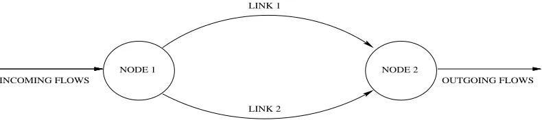
The problem of routing multiple flows in communication networks has been well studied during the last few decades (Bertsekas and Gallager, 1991) with several approaches having been proposed for static and dynamic optimization of routing. In Tsitsiklis and Bertsekas (1986) as well as Bertsekas and Gallager (1991), gradient based projection algorithms for optimal routing have been studied. More recently, in Marbach et al. (2000), Nowe et al. (1998) and Varadarajan et al. (2003), rein-forcement learning techniques have also been applied to the problem of routing. We consider here an application of our algorithm to finding optimal routes for flows in communication networks, conditioned on a rare event. The basic setting is shown in Fig. 1.

NODE 2 LINK 1

LINK 2

INCOMING FLOWS OUTGOING FLOWS

NODE 1

Figure 1: The Model

Nodes A and B are connected via two links. We assume that the system is slotted with time slots of equal length. Customers/flows arrive at the beginning of time slots at A, and have to be sent to

B. There are two routes R1and R2from A to B. An arrival occurs with a certain probability (p) in a given time slot independent of others. At the beginning of a time slot, decision on whether to route all arrivals (that occur in the time slot) onto R1or R2is made by a controller (at Node A). Thus, all new arrivals at the beginning of a time slot are routed either to R1or R2. However, we also assume that both R1and R2can accommodate at most M customers (or flows) at any given instant. All flows that cannot be accommodated in a given slot immediately leave the system. Suppose each flow at any given instant (or a slot boundary) finishes service w.p. q1on R1and w.p. q2on R2, respectively, independent of other flows. Further, if a flow does not finish service in a time slot, its service extends to the next slot independently of the number of flows in either route and the number of slots the given flow has been in service for. The above process is repeated again in subsequent slots. Thus the number of slots that a customer is in service at node j, j=1,2 equals i with probability (1−qj)i−1qj, for i≥1. Let Xn(1)(resp. Xn(2)) denote the number of flows on R1 (resp. R2) in time slot n. Let{A(n)}with A(n)∈ {a1,a2} ∀n≥1, denote the associated action-valued process, where

aicorresponds to the action of routing new flows in a time slot on the route Ri, i=1,2. Then under a given SDP,{Xn}, where Xn= (X(

1)

n ,Xn(2)), n≥0, forms a discrete time Markov chain with state transition equation given by

X_n(₊1)₁ X_n(₊2)₁

!

= min[X

(1)

n −Q1(n) +I{A(n) =a1}B(n),M] min[Xn(2)−Q2(n) +I{A(n) =a2}B(n),M]

!

where the departures from routes R1 and R2 during time slot n are denoted as Q1(n) and Q2(n), respectively, and satisfy 0≤Qj(n)≤Nj(n), j=1,2. Also, B(n)denotes the number of new arrivals at Node A, at the beginning of time slot(n+1). Note that since there are only two actions associated with each state here, the parameter vectorθi(n)of the randomized policy is simplyθi(n) =θ1i(n). The simplex Ti associated with each state here corresponds to the interval[0,1]∀i. The projection map Γi is thus defined by Γi(x) =max(0,min(x,1))∀i. Also, ¯θi(n) =Γi(θ1i(n) +δ41i(n)). The sequences{41

i(n), n≥0}, i∈S are generated using normalized Hadamard matrices. These turn out to be simply41

i(n) = (−1)n. The step-sizes are chosen as a(n) =b(n) =c(n) =1, n=0,1, and for n≥2,

a(n) =log(n)

n ,b(n) =

1

n,c(n) =

1

n log(n).

The single-stage cost in state i under policy ¯θi(n) is given by hθ¯i(n)(i,Xn+1) =|Xn(+1)1−N1| +|X_n(2₊)₁−N2|, where N1 and N2 are given thresholds and (as before) Xn+1 = (Xn(1+)1, X

(2)

n+1) corre-sponds to the state at the next instant. The cost function thus aims to keep the number of flows along R1to be near threshold N1and those along R2to be near N2for some 0≤N1, N2≤M. Here the parameters N1and N2 may be set arbitrarily. Note that since all new arrivals in a time slot are routed to either R1or R2, N1and N2should be judiciously chosen. A value of N1or N2close to zero would lead to under-utilization while a value close to M would result in leaving less room for ac-commodating future flows on the corresponding route. The latter is required, for instance, in cases where there are different categories of traffic flows in the network each having a possibly different pay off (a scenario not considered in this paper). Any other choice for the cost function may be used as well.

The function g·(·)used for defining the rare event is given as gθ¯Xn_(X

n) =I{X( 2)

n >N}, where N is another (given integer) threshold. Thus g·(·)equals one if Xn(2)∈ {N+1, . . . ,M}and is zero other-wise. The long-run average lim

n→∞ 1

n

n−1

∑

m=0

gθ¯Xm_(X

m)in this case corresponds to the stationary probability

of the number of flows at the second node exceeding N. For any given SDP, the latter quantity would depend on the resulting transition probability matrix for the process{Xn}under that SDP. We con-sider two different settings for our experiments that we refer to as settings (a) and (b), respectively. The input parameters for the two settings are given in Table 1 below.

Note that in the algorithm in Section 3.1, the number of iterations P is fixed apriori. However, for obtaining more accurate estimates, we use a different stopping criterion for the algorithm that is based on an accuracy parameterε as explained below and not one based on a fixed value of P. For a given ε>0, let kε be the transition number of the Markov chain at which the estimate of

ρµ∗

ζ ≡Vµ

∗

ζ (i0)converges to withinεof its previous value 100 times in succession. We let the value ofεto be 5×10−9 for setting (a) and 5×10−8 for setting (b), respectively. The above values of

ε(for the two settings) will in fact be denoted as ¯ε. More experiments using other values ofεare subsequently discussed.

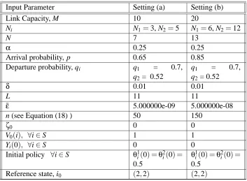
Input Parameter Setting (a) Setting (b)

Link Capacity, M 10 20

Ni N1=3, N2=5 N1=6, N2=12

N 7 13

α 0.25 0.25

Arrival probability, p 0.65 0.85 Departure probability, qi q1 = 0.7,

q2= 0.52

q1 = 0.7,

q2= 0.52

δ 0.01 0.01

L 11 11

¯

ε 5.000000e-09 5.000000e-08

n (see Equation (18) ) 50 150

ζ0 0 0

V0(i), ∀i∈S 1 1

Yi(0), ∀i∈S 0 0

Initial policy ∀i∈S θ1_i(0) =θ2 i(0) = 0.5

θ1

i(0) =θ2i(0) = 0.5

Reference state, i0 (2,2) (2,2)

Table 1: Input Parameters for the two settings

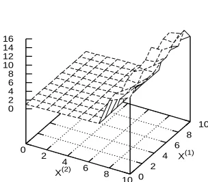
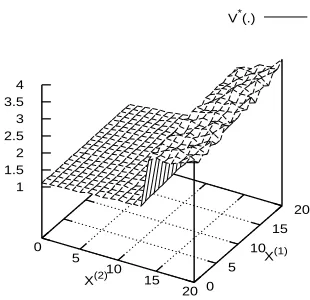
lines given the form of the associated cost function. The value function V∗(·) (in both settings) takes low values for low values of(i1,i2)and gradually increases (overall) when either i1 or i2 is increased. What is more interesting, however, is that there is a step-increase in these values as soon as the set of rare event states is reached and it stays high over those states. This is not surprising since the conditional probabilities of the rare event states will be higher as we are conditioning on the rare event.

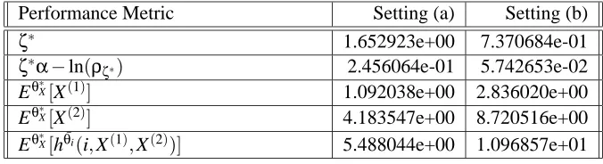
In Table 2, values of various performance metrics under the optimal policy are shown. Note that

ζ∗ _{corresponds to the converged value of the risk parameter obtained from the recursion (6). The} quantities Eθ∗X[X(1)]and Eθ∗X[X(2)]denote the mean numbers of flows on the two routes. These, in

general, depend on the parameters p, q1, q2, M andθ∗, and in the present case, can be seen to be less than the thresholds N1 and N2, in either setting. The mean cost Eθ∗X[_hθ¯i_(i,X(1)_,X(2)_{)], is higher in}

Setting (b) as compared to Setting (a) since the values of thresholds N1and N2in the former setting are higher.

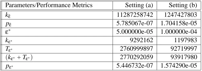
Next, we performed some additional experiments along similar lines as Borkar et al. (2004) and Bucklew (1990), to estimate the rare event probability ˆpn(see below) under the optimal policy for both settings. Note that even though our main aim is to obtain the optimal policy (above), the additional experiments provide insight on the choice of the accuracy parameterεand its effect on computational performance. We define

ˆ

pn=Px( 1

n

n−1

∑

m=0

θ* (.)

0 2

4 6

8 10

X(2) ₀ 2

4 6

8 10

X(1) 0.1

0.2 0.3 0.4 0.5 0.6 0.7 0.8 0.9

Figure 2: Setting (a): Optimal Policyθ∗(·)

V*(.)

0 2

4 6

8 10

X(2) ₀ 2

4 6

8 10

X(1) 0

2 4 6 8 10 12 14 16

θ* (.)

0 5

10 15

20

X(2) ₀

5 10

15 20

X(1) 0

0.1 0.2 0.3 0.4 0.5 0.6 0.7 0.8

Figure 4: Setting (b): Optimal Policyθ∗(·)

V*(.)

0 5

10 15

20

X(2) ₀

5 10

15 20

X(1) 1

1.5 2 2.5 3 3.5 4

Performance Metric Setting (a) Setting (b)

ζ∗ _{1.652923e+00 7.370684e-01}

ζ∗_α−ln(ρ

ζ∗) 2.456064e-01 5.742653e-02

Eθ∗X[X(1)] 1.092038e+00 2.836020e+00

Eθ∗X[_X(2)] _{4.183547e+00 8.720516e+00}

Eθ∗X[_hθ¯i_(i,X(1)_,X(2)_{)] 5.488044e+00 1.096857e+01}

Table 2: Performance under optimal policy

The values of n are described in Table 1 for the two settings. An importance sampling estimator for this probability is the average of the i.i.d. samples

I{1

n

n−1

∑

m=0

gθ∗(Xm)≥α}

pθ∗X0_(X0,X1)pθ∗X1_{(X1,X2)· · ·p}θ∗Xn−2(_Xn−2,_Xn−1)

pθ

∗

X0

∗ (X0,X1)p θ∗

X1

∗ (X1,X2)· · ·p θ∗

Xn−2

∗ (Xn−2,Xn−1)

.

In practice, one is able to obtain the above estimate only upto a certain specified degree of accuracy as obtained from the quantityε(see above). There is however a tradeoff involved in the choice of

ε. The variance of the estimates tends to be high ifεis not chosen to be small enough, which may affect their accuracy. On the other hand, as the value ofεis decreased beyond a point, the amount of computational effort required increases rapidly.

We run the algorithm for different values ofε. For each value ofε, we obtain an estimate pε_∗(·,·) of pθ_∗∗(·,·)that is then used to generate i.i.d. samples for the estimate of the rare event probability

ˆ

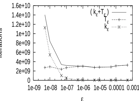
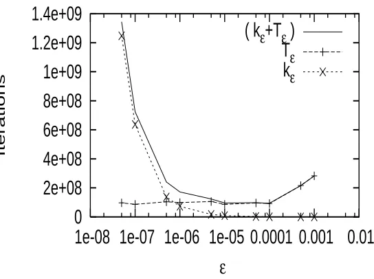
pn (see above). The mean and variance of the rare event probability are then determined using the batch means method. The simulation is terminated when the 95% confidence interval, see Law and Kelton (2000), of probability lies within 5% of its estimated mean value. Let Tε denote the total computational effort involved in terms of the number of simulated transitions of the MDP that are generated during this process. We show in Figs. 6 and 8, plots of k_ε, T_εand(k_ε+T_ε)as functions of

εfor settings (a) and (b), respectively. The total computational effort (in terms of(kε+Tε)) is found to be the least forε≡ε∗=5×10−5in setting (a) and forε≡ε∗=10−4in setting (b), respectively. Also, Figs. 7 and 9 show the plots of the rare event probability ˆpn (described in the figures as pε) obtained for different accuracy levelsε. The values ofεin the above figures are shown on the log scale for convenience.

0

2e+09

4e+09

6e+09

8e+09

1e+10

1.2e+10

1.4e+10

1.6e+10

1e-09 1e-08 1e-07 1e-06 1e-05 0.0001 0.001

Iterations

ε

( k

+T

)

T

k

Figure 6: Setting (a): Plot of k_ε,T_εand (k_ε+T_ε) w.r.t.ε

4.9e-07

5e-07

5.1e-07

5.2e-07

5.3e-07

5.4e-07

5.5e-07

5.6e-07

5.7e-07

5.8e-07

5.9e-07

1e-09 1e-08 1e-07 1e-06 1e-05 0.0001 0.001

Probability of Rare Event

ε

p

_ε

0

2e+08

4e+08

6e+08

8e+08

1e+09

1.2e+09

1.4e+09

1e-08 1e-07 1e-06 1e-05 0.0001 0.001 0.01

Iterations

ε

( k

+T

)

T

k

Figure 8: Setting (b): Plot of k_ε,T_ε and (k_ε+T_ε) w.r.t.ε

6e-06

8e-06

1e-05

1.2e-05

1.4e-05

1.6e-05

1.8e-05

1e-08 1e-07 1e-06 1e-05 0.0001 0.001 0.01

Probability of Rare Event

ε

p

Parameters/Performance Metrics Setting (a) Setting (b)

k¯ε 11287258742 1247427803

pε¯ 5.785067e-07 1.704158e-05

ε∗ _{5.000000e-05 1.000000e-04}

kε∗ 9292162 1197983

Tε∗ 2760999897 92719997

(k_ε∗ + T_ε∗) 2770292059 93917980

p_ε∗ 5.446732e-07 1.574290e-05

Table 3: Rare Event Probability Experiments

5. Conclusions

We developed an adaptive simulation based stochastic approximation algorithm for ergodic control of Markov chains conditioned on a rare event of zero probability. Our algorithm uses coupled re-cursions that are driven by different timescales. We briefly sketched the convergence analysis of our algorithm and presented numerical experiments on a setting involving routing multiple flows in com-munication networks. The results obtained demonstrate the usefulness of the proposed algorithm in obtaining optimal policies conditioned on a rare event and in estimating the rare event probability. The numerical setting considered here was, however, a simple setting designed to demonstrate the usefulness of the proposed algorithm. More complex settings involving, say, networks with multiple nodes and more routes with large numbers of flows on each should be tried in order to study the scalability of the proposed algorithm. The SPSA technique, in general, is known to be highly scal-able as has been demonstrated through several applications over the last decade. In the simulation based optimization framework, SPSA based multi-timescale algorithms have been found to perform well computationally in the case of high-dimensional parameter settings studied in Bhatnagar et al. (2001) and Bhatnagar et al. (2003) (by more than an order of magnitude over related K-W based algorithms). Implementations involving such high-dimensional settings (along the lines described above) need to be studied for the proposed algorithm in the setting of this paper. Recently, in Bhat-nagar (2005), certain Newton-based multiscale SPSA algorithms that estimate both the gradient and Hessian of the average cost have been developed in the simulation optimization setting. Similar algorithms for the setting considered here may also be developed.