Learning Coordinate Covariances via Gradients

Learning Coordinate Covariances via Gradients

Sayan Mukherjee [email protected]

Institute of Statistics and Decision Sciences Institute for Genome Sciences and Policy Department of Computer Science Duke University

Durham, NC 27708, USA

Ding-Xuan Zhou [email protected]

Department of Mathematics City University of Hong Kong

Tat Chee Avenue, Kowloon, Hong Kong, China

Editor: John Shawe-Taylor

Abstract

We introduce an algorithm that learns gradients from samples in the supervised learning framework. An error analysis is given for the convergence of the gradient estimated by the algorithm to the true gradient. The utility of the algorithm for the problem of variable selection as well as determining variable covariance is illustrated on simulated data as well as two gene expression data sets. For square loss we provide a very efficient implementation with respect to both memory and time.

Keywords: Tikhnonov regularization, variable selection, reproducing kernel Hilbert space,

gen-eralization bounds

1. Introduction

The advent of data sets with many variables or coordinates in the biological and physical sciences has driven the use of a variety of machine learning approaches based on Tikhonov regularization or global shrinkage such as support vector machines (SVMs) (Vapnik, 1998) and regularized least square classification (Poggio and Girosi, 1990). These algorithms have been very successful in both classification and regression problems. However, in a number of applications the classical questions from statistical linear modelling of which variables are most relevant to the prediction and how the coordinates vary with respect to each other have been revived. In the context of high dimensional data with few examples, the “large p, small n” paradigm (West, 2003), this leads to foundational questions in constructing and interpreting statistical models. Since statistical models based on shrinkage or regularization (Vapnik, 1998; West, 2003) have had success in the framework of both classification and regression, we formulate the problem of learning coordinate covariation and relevance in this framework.

1.1 Classification and Regression

Classification and regression problems can be addressed in the framework of learning or estimat-ing functions from a hypothesis space given sample values. An efficient learnestimat-ing method is the Tikhonov regularization scheme. Let X be a compact metric space and the hypothesis space,

H

, be a set of functions X _→Y _⊂R. If we assign a penalty functionalΩ:

H

_→R+ on

H

and choose a loss function V :R2→R+, the Tikhonov regularization scheme in

H

associated with(V,Ω)is

defined for a sample z=(xi,yi) m

i=1∈(X×Y)

m_{andλ>0 as}

f_zV =arg min

f_∈H

n₁

m

m

∑

i=1

V(yi,f(xi)) +λΩ(f)

o

. (1)

The efficiency of learning algorithms of type (1) in machine learning can be seen when

H

takes the special choice of a reproducing kernel Hilbert space generated by a Mercer kernel.

Let K : X_×X_→Rbe continuous, symmetric and positive semidefinite, i.e., for any finite set of distinct points_{x1,_···,xm} ⊂X , the matrix(K(xi,xj))mi,j=1is positive semidefinite. Such a function is called a Mercer kernel.

The reproducing kernel Hilbert space (RKHS)

H

_K associated with the Mercer kernel K is defined (see Aronszajn (1950)) to be the completion of the linear span of the set of functions {Kx:=K(x,·): x∈X}with the inner producth·,·iKsatisfyinghKx,KyiK=K(x,y).The reproducing

property of

H

_Kis

hKx,fiK= f(x), ∀x∈X,f ∈

H

K. (2)

If

H

=

H

_KandΩ(f) =_kf_k2_Kin (1), the reproducing property (2) tells us that f_zV =

m

∑

i=1 ciKxi

and the coefficients_{ci}m_i=1can be found by solving an optimization problem inRm.

Assume thatρis a probability distribution on Z :=X_×Y and z=(xi,yi) m i=1∈Z

m_{is a random}

sample independently drawn according toρ.

When the loss function is the least-square loss V(y,t) = (y₋t)2_{, the algorithm (1) is least-square} regression and the objective is to learn the regression function

f_ρ(x) =

Z

Y

ydρ(y_|x), x_∈X (3)

from the random sample z. Hereρ(_·|x) is the conditional distribution ofρat x. DenoteρX as the marginal distribution ofρon X and L2_ρX as the L2space with the metric_kf_kρ:= (R

X|f(x)|2dρX)1/2.

There has been a vast literature (e.g. (Evgeniou et al., 2000; Zhang, 2003; Vito et al., 2005; Smale and Zhou, 2006b)) in learning theory showing for this least-square regression algorithm the con-vergence of f_zV to fρin the metric_{k · k}ρunder the assumption that fρlies in the closure of

H

_Kand

λ=λ(m)_→0 as m_→∞.

For the (binary) classification purpose, we take Y =_{1,₋1_}. A real valued function f : X_→R

induces a classifier sgn(f): X→Y . In this case, one uses a (convex) loss functionφ:R→R+to

measure the empirical errorφ(t), t=y f(x), when sgn(f(x))is applied to predict y_∈Y . Examples of such a convex loss functionφinclude the logistic loss

and the hinge loss φ(t) =max{0,1−t}. For V(y,f(x)) =φ(t) in (1) extensive investigation in learning theory (e.g. (Cortes and Vapnik, 1995; Evgeniou et al., 2000; Schoelkopf and Smola, 2001; Vapnik, 1998; Wu and Zhou, 2005)) has shown that sgn(f_zV) converges to the Bayes rule sgn(fρ)with respect to the misclassification error:

R

(sgn(f)) =Prob_{sgn(f(x))₆=y_}.

1.2 Learning the Gradient

In this paper we are interested in learning the gradient of fρfrom the function sample values. Let X _⊂Rn. Denote x= (x1,x2, . . . ,xn)T _∈Rn_{. The gradient of f}

ρ is the vector of functions (if the partial derivatives exist)

∇f_ρ=

_∂ fρ

∂x1, . . . ,

∂fρ

∂xn

T

. (5)

The relevance of learning the gradient with respect to the problems of variable selection and estimating coordinate covariation is that the gradient provides the following information:

(a) variable selection: the norm of a partial derivative_k∂_∂f_xρikindicates the relevance of this variable,

since a small norm implies a small change in the function f_ρwith respect to the i-th coordinate,

(b) coordinate covariation: the inner product between partial derivatives D_∂f

ρ

∂xi,

∂fρ

∂xj

E

indicates the covariance of the i-th and j-th coordinates with respect to variation in f_ρ.

We now motivate the derivation of our gradient learning algorithm. Taylor expanding a function g(u)around the point x gives us

g(u)_≈g(x) +

Z

∆x∈Γx

h∇g,∆x_i,

where the inner product and a neighborhoodΓxof x are determined according to what is natural for different settings. For example, in the manifold setting we know the marginalρX is concentrated on a manifold

M

and it is natural to formulate the following expansion

g(u)_≈g(x) +

Z

∆x∈Mx

h∇Mg,∆xi,

where ∆x_∈

M

_x are points on the manifold around x with respect to the intrinsic distance on the manifold and the inner product is L2 over the manifold (Belkin and Niyogi, 2004). In the graph setting we are given a sparse sample on the manifold which can be thought of as vertices of a graph and the distance between the points is the weight matrix of the graph. A natural for-mulation in this setting is to set Γx to be vertices connected to x and the inner product as the weight matrix. Minimizing the empirical error (with regularization) between g(u) and its expan-sion g(x) +R

∆x_∈Γxh∇g,∆xi ≈g(x) +∇g(x)·(u−x)for u≈x results in various learning algorithms.

For regression the algorithm to learn gradients will use least-square loss to minimize the error of the Taylor expansion at sample points. To learn vectors of functions we use the hypothesis space

H

n

K which is an n-fold of

H

K: each~f ∈

H

Kn can be written as a column vector of functions

~_{f = (f1,f2, . . . ,fn)}T _{with f}

ℓ∈

H

K. Defineh~f,~hiK=∑n_ℓ=1hfℓ,hℓiK. Thenk~fk2K =∑nℓ=1kfℓk2K. The

empirical error on sample points x=xi,u=xjwill be measured by the square loss

g(u)₋g(x)₋∇g(x)_·(u₋x)2= yi−yj+~f(xi)·(xj−xi)

The restriction u_≈x will be enforced by weights: wi,j =w(s)i,j >0 corresponding to (xi,xj) with

the requirement that w(s)_{i,j →}0 as_|xi−xj|/s→∞. For x= (x1,x2, . . . ,xn)T ∈Rn, we denote |x|= ∑n

j=1(xj)2 1/2

.

One possible choice of weights is given by a Gaussian with variance s. Let w =ws be the

function onRngiven by w(x) =_sn1+2e−

|x|2

2s2. Then this choice of weights is

wi,j=w(s)i,j =

1 sn+2e

−|xi−x j|

2

2s2 =w(x_i−x_j), i,j=1, . . . ,m. (6)

For regression we define the algorithm by the following optimization problem with weights being arbitrary positive numbers wi,j=w(s)i,j which depend on an index s>0.

Definition 1 The least-square type learning scheme is defined for the sample z_∈Zmas

~_{fz,λ:=arg min} ~_f∈Hn K

1 m2

m

∑

i,j=1 w(s)_i,j

yi−yj+~f(xi)·(xj−xi)

2

+λ_k~fk2

K

, (7)

whereλ,s are two positive constants called the regularization parameters.

A similar algorithm can be defined for classification with a convex loss functionφ(_·)like the hinge or logistic loss.

Definition 2 The regularization scheme for classification is defined for the sample z∈Zmas

~_{fz,λ=arg min} ~_f∈Hn K

1 m2

m

∑

i,j=1 w(s)_i,jφ

yi yj+~f(xi)·(xi−xj)

+λ_k~f_k2_K

. (8)

Remark 3 Some algorithms for computing numerical derivative by means of partition were intro-duced in Wahba and Wendelberger (1980). They work well in low dimensional spaces. In high dimensional spaces, partition is difficult. Our method can be regarded as an algorithm for numeri-cal derivatives in high dimensional spaces.

At first thought, a natural approach to computing partial derivatives would be to estimate the regression function and then compute partial derivatives. The problem with this approach is that the partial derivatives are no longer in the RKHS of the regression function. This leaves us with the problem of not having a norm or computable metric to work with. The advantage of our method is the derived functions are already approximations of the partial derivatives and they have RKHS inner products which are computed in the estimation process. The inner products reflect the nature of the measure, which is often on a low dimensional manifold embedded in a large dimensional space.

The hypothesis space

H

n

K in the optimization problem (7) may be replaced by some other space

of vector-valued functions (Micchelli and Pontil, 2005) in order to learn the gradients.

1.3 Overview

In Sections 2 and 3, we shall derive linear systems for solving the optimization problem (7). In particular, when m<<n, an efficient algorithm will be provided.

The regularization parameters in (7) depend on m:λ=λ(m), s=s(m)and generallyλ(m),s(m)_→

0 as m becomes large. In Section 4, we show for a Gaussian weight function (6) how a particular choice of the two regularization parameters leads to rates of convergence of our estimate of the gradient to the true gradient,~fz,λto∇fρ.

The utility of the algorithm is demonstrated in Section 5 in applications to simulated data as well as gene expression data. We close with a brief discussion in Section 6.

2. Representer Theorem

The optimization problem defining the least-square algorithm (7) can be solved as a linear sys-tem of equations. Denote Rp×q as the space of p_×q matrices, In the n×n identity matrix, and

diag_{B1,B2,···,Bm}the m×m block diagonal matrix with each Bi∈Rn×n. To save space, we

ex-press an mn column vector with blocks_{ci∈Rn}by the following abuse of notion c= (c1,c2, . . . ,cm)T.

The following theorem is an analog of the standard representer theorem (Schoelkopf and Smola, 2001) that states the minimizer of the optimization problem defined by (7) has the form

~_fz,λ=

∑

m

i=1

ci,zKxi (9)

with cz= (c1,z, . . . ,cm,z)T∈Rmn. Theorem 5 For i=1, . . . ,m,let Bi

Bi= m

∑

j=1

wi,j(xj−xi)(xj−xi)T∈Rn×n, Yi= m

∑

j=1

wi,j(yj−yi)(xj−xi)∈Rn. (10)

Then~fz,λ=∑mi=1ci,zKxi with cz= (c1,z, . . . ,cm,z)

T_∈Rmn_{satisfying the linear system}

m2λImn+diag{B1,B2,···,Bm}

K(xi,xj)In

m i,j=1

c= (Y1,Y2, . . . ,Ym)T. (11)

Proof By projecting onto the span of _{Kxi}

m

i=1 the reproducing property (2) ensures that ~fz,λ=

∑m

i=1ci,zKxi,with ci,z∈R

n_{for each i.Note that x·v=∑}n

i=1xivi=xTv for x,v∈Rn. To find{ci,z},

we consider~f =∑m

i=1ciKxi ∈

H

n

K with ci∈Rn.Then

~_{f(xi)·(xj−xi) =}

∑

m

p=1

K(xp,xi)cp·(xj−xi) = m

∑

p=1

K(xp,xi)(xj−xi)Tcp

and

k~f_k2_K= m

∑

i,j=1

K(xi,xj)ci·cj.

Define the empirical error

E

_zas

E

_z(~f) = 1

m2

m

∑

i,j=1 w(s)_i,j

yi−yj+~f(xi)·(xj−xi)

It is a function of mn variables{ck_q: 1≤q≤m,1≤k≤n}where the q-th coefficient cq∈Rn of~f

is expressed as(ck_q)n

k=1= (c1q, . . . ,cnq)T. For q∈ {1, . . . ,m},k∈ {1, . . . ,n}, ∂

∂ck q

n

E

z(~f) +λ_k~f_k2_K o

=2λ

m

∑

i=1

K(xq,xi)cki

+ 2

m2

m

∑

i,j=1

wi,j yi−yj+ m

∑

p=1

K(xp,xi)(xj−xi)Tcp

!

K(xq,xi)(xkj−xki).

Notice from (2) that for g,h_∈span_{Kxi}

m

i=1, g(xi)−h(xi) =0 for i=1, . . . ,m implies that g−h

is orthogonal to each Kxi, and hence g−h=0. Then we know that ~fz,λ=∑

m

i=1c˜i,zKxi where ˜cz=

{c˜i,z}m_i=1is the solution to the linear system

λci+

1 m2

m

∑

j=1

wi,j yi−yj+ m

∑

p=1

K(xp,xi)(xj−xi)Tcp

!

(xj−xi) =0,i=1, . . . ,m.

Since(xj−xi)Tcp is a scalar,[(xj−xi)Tcp](xj−xi) = (xj−xi)(xj−xi)Tcp. So the above system

can be expressed as

Bi m

∑

p=1

K(xi,xp)cp+m2λci=Yi, i=1, . . . ,m. (12)

This is exactly the system in (11).

Remark 6 One might consider solving the optimization problem (7) by finding each component of ~_fz

,λ separately. However, to find(~fz,λ)ℓ by minimizing over f ∈

H

K, one needs to replace yi−yj

by yi−yj+∑k=₆ ℓ(~fz,λ)k(xi)(xkj−xik). So the optimization problems for components of ~fz,λare not completely separable. It would be interesting to have a separable method for (7).

3. Reducing the Matrix Size

In some applications of variable selection, the number n of variables is much larger than the sample size m. In such a situation, the system (11) for implementing the learning algorithm (7) is not satisfactory, since the size of the linear system (11) is(mn)_×(mn).

Observe that each term in the summation defining Bi in (10) is a rank one matrix. Hence the

rank of the n_×n matrix Biis at most m for each i. This raises the expectation of reducing the matrix

size in the linear system (11). In this section, we show how to reduce this size to(

S

m)_×(

S

m)with

S

_≤m₋1. Moreover, an approximation algorithm will be introduced which is often implemented with

S

<<m.

We use the well known approach of singular value decomposition. It may be applied to the coefficient matrix of (11) to reduce the matrix size. Here we prefer to apply the approach to a matrix involving the data only, leaving us flexibility for the weights wi,j.

Consider the matrix involving the data x given by

Mx= [x1−xm,x2−xm, . . . ,xm−1−xm,xm−xm]∈Rn×m. (13)

Assume the rank of Mxis d. Then d≤min{m−1,n}since the last column of the matrix is zero.

V = [V1,V2, . . . ,Vn]and a m×m orthogonal matrix U= [U1,U2, . . . ,Um]such that

Mx=VΣUT= [V1V2 ···Vn]

diag_{σ1,σ2,···,σd} 0

0 0     

U₁T U₂T .. . U_mT

   

. (14)

Hereσ1≥σ2≥ ··· ≥σd>σd+1=. . .=σmin{m,n}=0 are the singular values of Mx. The matrixΣ

is n_×m and has entries zero except that(Σ)i,i=σi for i=1, . . . ,d. From expression (14), we see

that

Mx= d

∑

ℓ=1

σℓVℓU_ℓT.

Note that U_ℓT = [U_ℓ1, . . . ,U_ℓm]. The j-th column of Mxequals xj−xm=∑dℓ=1σℓVℓU

j

ℓ and xj−xi=

d

∑

ℓ=1

σℓ

U_ℓj₋U_ℓiVℓ. (15)

It follows that Yi=∑mj=1wi,j(yj−yi)∑dℓ=1σℓ

U_ℓj₋U_ℓi

Vℓand

Bi= m

∑

j=1 wi,j

d

∑

ℓ=1

d

∑

p=1

σℓσp

U_ℓj₋U_ℓi

U_pj₋U_piVℓVpT. (16)

Now we can reduce the matrix size by solving an approximation to the linear system derived from the singular values. A strong correlation among the vectors_{xi}would result in a large number

of small singular values. If we ignore the small singular valuesσS+1, . . . ,σd, the error is proportional toσS+1. This follows from the idea of low-rank approximations in singular value decomposition.

The following theorem quantifies the above statement.

Theorem 7 Assume_|y_{| ≤}M almost surely. Denoteκ=sup_x∈XpK(x,x). Let 1_≤

S

_≤d. Set

B

_i= m

∑

j=1 wi,j

h

σℓσp

U_ℓj₋U_ℓi U_pj₋U_pii

S

ℓ,p=1∈R

S_×S_{, i=1, . . . ,m (17)}

and

Y

_i= m

∑

j=1

wi,j(yj−yi)

h

σℓ

U_ℓj₋U_ℓi iS

ℓ=1∈R

S_{, i=1, . . . ,m. (18)}

Solve the linear system n

m2λImS+diag{

B

1,···,

B

m}

K(xi,xj)IS

m i,j=1

o

ˆb= (

Y

₁, . . . ,

Y

_m)T_{. (19)}

The solution ˆbz = (ˆb1,z, . . . ,ˆbm,z)T ∈RmS gives an approximation ~fz,λ,S =∑m_i=1bi,zKxi with bi,z=

∑S

ℓ=1ˆbℓi,zVℓ. The error between bz= (bi,z)mi=1and czcan be bounded as

bz−cz

ℓ2_(Rmn₎≤

4MσS+1 m2λ

p

d∆m+2κ

2σ2 1 mλ √

S

∆m , (20)

where∆m:=max1≤i≤m ∑mj=1wi,j

2

+∑m i,j=1 wi,j

See Appendix B for the proof.

If we set

S

=d, we can solve for~fz,λexactly with a linear system of reduced size. This is stated in the following corollary.

Corollary 8 Letσ1≥σ2≥ ··· ≥σd >0 be all the positive singular values of Mxand U,V be the

orthogonal matrices in (14). Then~f_z,λ=∑m i=1

∑d

ℓ=1ceℓi,zVℓ Kxi whereecz satisfies (19) with

B

iand

Y

_igiven by (17) and (18) with

S

=d, respectively.

Theorem 7 provides a theoretical foundation for the following approximation algorithm with reduced matrix size that accurately approximates~fz,λby~fz,λ,S.

3.1 Reduced Matrix Size Algorithm

The following is an outline of the reduced matrix algorithm. See appendix C for Matlabr code implementing this algorithm.

Algorithm 1: Approximation algorithm with reduced matrix size to approximate~fz,λ input : inputs(xi)mi=1, labels(yi)mi=1, kernel K, weights(wi,j), eigenvalue thresholdε>0

return: coefficients(bi,z)mi=1

Mx= [x1−xm,x2−xm, . . . ,xm−1−xm,xm−xm]∈Rn×m;

Given Mxcompute the singular value decomposition (14) with orthogonal matrices U,V and

singular valuesσ1≥σ2≥ ··· ≥σS >ε;

tj= σ1U₁j, . . . ,σSU_SjT∈RS for 1≤ j≤m;

B

_i=∑m

j=1wi,j(tj−ti)(tj−ti)T for 1≤i≤m;

Y

_i=∑m

j=1wi,j(yj−yi)(tj−ti)for 1≤i≤m;

e K=

    

B

1K(x1,x1)

B

1K(x1,x2) _···

B

1K(x1,xm)

B

2K(x2,x1)

B

2K(x2,x2) _···

B

2K(x2,xm)

..

. . .. ··· ...

B

mK(xm,x1)

B

mK(xm,x2) ···

B

mK(xm,xm)

    ,

~

Y

=

    

Y

₁

Y

2 .. .

Y

m

    

ˆbz= (ˆb1,z, . . . ,ˆbm,z)T∈RmS where

m2λImS +Ke

ˆbz=~

Y

(21)

bi,z=∑S_ℓ=1ˆbℓi,zVℓand~fz,λ,S =∑mi=1bi,zKxi is an approximation of~fz,λ;

4. Error Analysis

In what follows we use Gaussian weights (equation (6)) and estimate error bounds. We show that ~_fz

,λ→ ∇fρ as m→ ∞ for suitable choices of the regularization parameters going to zero, λ=

λ(m)_→0,s=s(m)_→0. Since we are learning gradients, some regularity conditions on both the marginal distribution and the density are required. The following case illustrates the idea (this case corresponds to the realizable setting in the PAC learning paradigm and will be a corollary of the error analysis that follows).

Proposition 9 Assume _|y_{| ≤}M almost surely. Suppose that for some 0<τ_≤2/3,c_ρ>0, the marginal distributionρX satisfies

ρX {x_∈X : inf

u∈Rn_\X|u−x| ≤s}

≤c2_ρs4τ, _∀s>0, (22)

and the density p(x)of dρX(x)exists and satisfies

sup

x∈X

p(x)_≤cρ, _|p(x)₋p(v)_{| ≤}cρ|v₋x_|τ, _∀v,x_∈X. (23)

Chooseλ=λ(m) =m−n+2τ+3τ and s=s(m) = (κc_ρ) 2

τ_m−n+21+3τ. If∇f_ρ∈

H

n

K and the kernel K is C3,

then there is a constant C_ρ,K such that for any 0<δ<1 and m≥1, with confidence 1−δ, we have

k~fz,λ−∇fρkρ≤Cρ,Klog

2

δ

1 m

₋ τ

2(n+2+3τ)

. (24)

The condition (23) means the density of the marginal distribution is H¨olderτ. The condition (22) is about the behavior ofρX near the boundary of X . They are natural assumptions for learning gradients of the regression function. When the boundary is piecewise smooth, (23) implies (22).

The idea behind the proof for the convergence of the gradient consists of simultaneously con-trolling a sample or estimation error term and a regularization or approximation error term. The first term, the sample error, is bounded using a concentration inequality since it is a function of the sample, z. The second term, the regularization error, does not depend on the sample and we use functional analysis to bound this quantity.

4.1 Sample Error

First we estimate the sample error by means of the sampling operator introduced in Smale and Zhou (2004, 2006b,a).

Definition 10 The sampling operator Sx:

H

Kn→Rmnassociated with a discrete subset x={xi}m_i=1

of X is defined by

Sx(~f) = ~f(xi)m_i=1= ~f(x1), . . . , ~f(xm)T. The adjoint of the sampling operator, ST_x :Rmn→

H

n

K, is given by

S_xTc= m

∑

i=1

ciKxi, c= (ci)

m

Denote Dx=diag{B1,B2,···,Bm}and~Y = (Y1,Y2, . . . ,Ym)T.

Consider equation (12) satisfied by cz. The quantity ∑mp=1K(xi,xp)cp,z equals~fz,λ(xi). Then (12) implies ST_xDxSx+m2λI

_~

fz,λ=STx~Y . Therefore,

~_fz,λ= 1 m2S

T

xDxSx+λI

₋1 ₁ m2S

T

x~Y. (25)

We introduce an s-generalization error corresponding to the empirical error as follows.

Definition 11 The s-generalization error

E

=

E

_sis defined for vectors of functions as

E

(~f) =

Z

Z

Z

Z

w(x₋u)

y₋v+~f(x)_·(u₋x)

2

dρ(x,y)dρ(u,v).

If we denoteσ2

s =

Z

Z

Z

Z

w(x₋u)(y₋f_ρ(x))2_{dρ(x,y)dρ(u,v), then}

E

(~f) =2σ2_s+

Z

X

Z

X

w(x₋u)

fρ(x)₋fρ(u) +~f(x)_·(u₋x)

2

dρX(x)dρX(u). (26)

A data independent limit of~fz,λis

~_{fλ=arg min} ~f_∈Hn K

E

(~f) +λ_k~f_k2_K . (27)

Taking the functional derivatives, we know from (26) that ~f_λ can be expressed in terms of the following integral operator on the space L2

ρX

n

with norm_k~f_kρ= _kf_ℓk2

ρ1/2.

Proposition 12 Let LK,s: L2_ρX

n

→ L2_ρXnbe the integral operator defined by

LK,s~f=

Z

X

Z

X

w(x₋u)(u₋x)Kx(u−x)T~f(x)dρX(x)dρX(u). (28)

It is a positive operator on L2_ρXnand

~_{fλ= LK,s+λI}−1_~

f_ρ,s. (29)

where

~_fρ,s:=Z

X

Z

X

w(x₋u)(u₋x)Kx fρ(u)−fρ(x)

dρX(x)dρX(u). (30)

The operator LK,shas its range in

H

Kn. It can also be regarded as a positive operator on

H

Kn. We

shall use the same notion for the operators on these two different domains.

Proposition 13 Let z=_{zi}m_i=1be i.i.d. draws from a probability distributionρon Z,(H,k · k)be a Hilbert space, and F : Zm_→H be measurable. If there isMe_≥0 such that_kF(z)₋Ezi(F(z))k ≤Me

for each 1_≤i_≤m and almost every z_∈Zm, then for everyε>0,

Probz_∈Zm{kF(z)−Ez(F(z))k ≥ε} ≤2 exp

− ε

2 2(Meε+σ2₎

, (31)

whereσ2:=∑m

i=1supz_\{zi}∈Zm−1Ezi{kF(z)−Ezi(F(z))k

2_{}. For any 0<δ<1, with confidence 1−δ,} there holds

kF(z)₋Ez(F(z))k ≤2 log

2

δ

e

M+√σ2 _.

Proof Apply Theorem 3.3 of Pinelis (1994) (see Appendix A) to the finite sequence_{fj=Ezm,...,zjF−

Ezm,...,z1F : j=1,2, . . . ,m+1}. So f1=0 and fm+1=F(z)−Ez(F(z)). Note thatkfj−fj−1k ≤Me

almost surely and∑m+_j=21Ezj−1kfj−fj−1k

2_≤σ2_{. The conditions of Theorem 3.3 of Pinelis (1994)} hold with B2=σ2_{,Γ=M. As pointed out in a correction of Pinelis (1999), the probability shoulde} be 2 exp₋ r2

rΓ+B2_+B√_B2_+2rΓ , which is bounded by 2 exp

−2(rΓr+B2 2₎ . Inequality (31) follows from

the theorem.

Chooseεsuch that ε2

2Meε+2σ2 =log

2

δ. That is,εsatisfies

ε2_{=2M loge} 2

δε+2σ2log

2

δ.

Therefore, with confidence at least 1₋δ, we have

kF(z)₋Ez(F(z))k ≤ε≤2M loge

2

δ+

r

2σ2_log2

δ ≤2 log

2

δ

_e

M+√σ2 _. This proves the proposition.

Now we can give the main result on the sample error_k~fz,λ−~fλkK. Denote the diameter of X as

Diam(X) =maxx,t_∈X|x−t|and the moments of the Gaussian as

Jp:=

Z

Rne

−|x2|2|x|pdx, p≥0.

In the following sample error estimates, the bounds are valid for any m,λ, and s, though they yield reasonable learning rates only for suitable choices ofλ=λ(m) and s=s(m) which we state in Proposition 9.

Theorem 14 Assume_|y_{| ≤}M almost surely.

1. For any 0<δ<1, with confidence 1₋δ, we have

k~fz,λ−~fλkK≤

16κDiam(X)log(2/δ) √

mλsn+2

2M+κDiam(X)_k~f_λkK

+1

mk~fλkK. (32)

2. If the density p(x)of dρX(x)exists and satisfies sup_x∈Xp(x)_≤cρ, then for any 0<s_≤1, with confidence 1₋δ, there holds

k~fz,λ−~fλkK ≤

8κlog(2/δ) √

mλs1+n/2

√_c

ρ+√Diam(X)

ms1+n/2

2M√J2+κ(Diam(X) +√J4)_k~f_λkK

+1

Proof By (25), we have

~_fz,λ−~_fλ= 1 m2S

T

xDxSx+λI

₋1 1 m2S

T x~Y−

1 m2S

T

xDxSx~fλ−λ~fλ

.

Define a vector-valued function F : Zm_→

H

n K by

F(z) = 1

m2S

T x~Y−

1 m2S

T

xDxSx~fλ.

That is,

F(z) = 1

m2 m

∑

i=1 m

∑

j=1

wi,j(xj−xi)Kxi(yj−yi)−

1 m2 m

∑

i=1 m

∑

j=1

wi,j(xj−xi)Kxi(xj−xi)

T_~f

λ(xi).

By independence, the expected value of F(z)equals

1 m2

m

∑

i=1 Ezi

∑

j6=i

Ezj

wi,j(xj−xi)Kxi

(yj−yi)−(xj−xi)T~fλ(xi)

= m−1

m2

m

∑

i=1 Ezi

Z

X

w(xi−u)(u−xi)Kxi

(f_ρ(u)₋yi)−(u−xi)T~fλ(xi)

dρX(u)

.

It follows that

Ez(F(z)) =

m₋1 m ~fρ,s−

m₋1 m LK,s~fλ.

By (29), LK,s~fλ+λ~fλ=~fρ,s. Henceλ~fλ=~fρ,s−LK,s~fλ=_mm₋₁Ez(F(z)). Therefore,

k~f_z,λ−~f_λkK≤

1

λkF(z)−

m

m−1Ez(F(z))kK≤ 1

λkF(z)−Ez(F(z))kK+

1 mk

~_fλkK.

The reproducing property (2) together with the upper boundκimplies

kfkρ≤ kfk∞≤κkfkK, ∀f∈

H

K. (34)

Then we apply Proposition 13 to the function F(z)to get our error bound. Let i_{∈ {}1, . . . ,m_}. We know that F(z)₋Ezi(F(z))equals

1 m2

∑

j₆=i

w(xi−xj)(xj−xi)

Kxi

yj−yi−(xj−xi)T~fλ(xi)

+Kxj

yj−yi−(xj−xi)T~fλ(xj)

− 1 m2

∑

j6=i

Z

Xw

(x−xj)(xj−x)

Kx

yj−fρ(x)−(xj−x)T~fλ(x)

+Kxj

yj−fρ(x)−(xj−x)T~fλ(xj)

dρX(x).

Using (34) for~f_λand_|x₋xj| ≤Diam(X)for any x∈X , we see that

kF(z)₋Ezi(F(z))kK≤Me=

4κDiam(X)

msn+2

2M+κDiam(X)_k~f_λkK

1. We first prove (32). Apply the trivial boundσ2≤mMe2. Then Proposition 13 tells us that for any 0<δ<1, with confidence 1₋δ, there holds

kF(z)₋Ez(F(z)kK≤2 log

2

δ

e

M+√mMe _≤4 log2

δ√mMe.

This proves (32).

2. To prove (33) we need to improve on our estimate of the variance σ2, we bound _kF(z)₋

Ezi(F(z))kKby

1 m2

∑

j6=i

w(xi−xj)|xj−xi|

2κ2M+2_|xj−xi|κ2k~fλkK

+ 1

m2

∑

j6=i

Z

X

w(x₋xj)|xj−x|

2κ2M+2_|xj−x|κ2k~fλkK

dρX(x).

It follows that Ezi(kF(z)−Ezi(F(z))k

2

K)

1/2

is bounded by

2 m2

∑

j6=i

Z

X

w(x₋xj)2_|xj−x|2

4κM+2_|xj−x|κ2k~fλkK

2 dρX(x)

1/2

≤_m2₂

∑

j6=i

_Z

X

s−2(n+2)e−

|x−x j|2

s2 |x_j−x|24κM 2c_ρdx

1/2

+ 2

m2

∑

j6=i

Z

X

s−2(n+2)e−

|x−x j|2

s2 |x_j−x|4(2κ2)2k~f_λk2_Kc_ρdx

1/2 .

Here we have used the assumption dρX(x) =p(x)dx with p(x)_≤cρ. Bounding the above integrals by those on the whole spaceRn, we see from the definition of the moments Mrthat

Ezi(kF(z)−Ezi(F(z))k

2

K)≤

2(m₋1)

m2

4κM√cρ

r J2

sn+2₂1+n/2+2κ 2

k~f_λkK√cρ

r J4 sn₂2+n/2

.

It follows then that for s_≤1

σ2_≤16cρκ2 msn+2

21/4M√J2+κk~fλkK

√ J4

2 .

The second statement (inequality (33)) follows from Proposition 13.

4.2 Regularization Error

In this subsection, we shall bound the regularization error _k~f_λ−∇fρk by a functional analysis approach. To illustrate the idea, we state the result for a special case when ∇f_{ρ ∈}

H

n

K. It is a

corollary of Theorem 17 and Theorem 19 with r=1/2.

Proposition 15 Assume (22) and (23). Denote V_ρ=R

X(p(x))2dx>0. Suppose that∇fρ∈

H

Knand

for some c′_ρ>0,

Then for anyλ>0 and 0<s_≤min2κ2c_ρ M2+τ+J4+cρJ2

1/τ_λ1/τ

,1 , there holds

k~f_λ−∇fρkρ≤ κ2c′_ρJ3s

λ+

2 Vρn(2π)n/2−1/2_k∇fρkK

√

λ.

To estimate the regularization error, we need to consider the convergence of Lk,sas s→0.

Lemma 16 Assume that for some 0<τ<1, conditions (22) and (23) hold. Then V_ρ≤c_ρand for any 0<s_≤1 we have

kLK,s−Vρn(2π)n/2LKkHn

K→HKn ≤s

τ_κ2_c

ρ M2+τ+J4+cρJ2

, (36)

where LKis a positive operator on

H

Kndefined by

LK~f =

Z

X

Kx~f(x)

p(x)

Vρ dρX(x). (37)

The operator LKis also a positive operator on(L2_ρX)

n_satisfying

kLK,s−Vρn(2π)n/2LKk(L2

ρX)

n_→(L2

ρX)

n ≤sτκ2cρ M2₊τ+J4+cρJ2

, _∀0<s≤1. (38)

Proof Let~f _∈(L2_ρX)2_{. Denote} ~g=

Z

X

Z

X

w(x₋u)(u₋x)Kx(u−x)Tdu

p(x)~f(x)dρX(x).

Then by (23) and the Cauchy-Schwartz inequality we see that_kLK,s~f−~gkK is bounded by

Z

X

_Z

X

1 sne

−|u_2s2−x|2u−x s

2

kKxkKcρ|u−x|τdu

~_f(x)dρX(x)_≤sτκc_ρM2+τk~fkρ.

Observe that n(2π)n/2=J2andR

Rnw(u−x)(ui−xi)(uj−xj)du=0 when i6= j. Then

R Rn_s1ne−

|u−x|2

2s2 u−x

s

_u−x

s

T

du=J2In. Hence

Vρn(2π)n/2LK~f =

Z

X

Z

Rn

1 sne

−|u_2s2−x|2 u−x s

u₋x s

T

du

p(x)Kx~f(x)dρX(x).

It follows that

k~g₋V_ρn(2π)n/2LK~fkK =

Z X Z

Rn_\X

1 sne

−|u−_2s2x|2 u−x s

u₋x s

T

du

p(x)Kx~f(x)dρX(x)

K ≤ Z X _Z

Rn_\X

1 sne

−|u−_2s2x|2u−x s

2

du

κ|~f(x)_|p(x)dρX(x).

Separate the domain X into Xs:={x∈X : infu∈Rn_\X |u−x| ≤√s}, consisting of those points

whose distance to the boundary is at most√s, and its complement X_\Xs.

If x_∈X_\Xs, any u∈Rn\X satisfies|u−x| ≥√s and thereby 1≤s

u₋x

s

2

. Hence

Z

Rn_\X

1 sne

−|u−_2s2x|2u−x s

2

du_≤s Z

Rn_\X

1 sne

−|u_2s2−x|2u−x s

4

It follows from (23) that

Z

X\Xs

Z

Rn_\X

1 sne

−|u_2s2−x|2u−x s

2

du

κ|~f(x)_|p(x)dρX(x)_≤sκcρM4 Z

X\Xs

|~f(x)_|dρX(x)

which is bounded by sκcρM4_k~f_kρ.

For the subset Xs, we use the Cauchy-Schwartz inequality and (23) to obtain

Z

Xs

_Z

Rn_\X

1 sne

−|u−_2s2x|2u−x s

2

du

κ|~f(x)_|p(x)dρX(x)_≤

Z

Xs

κc_ρM_2|~f(x)_|dρX(x).

This is bounded byκc_ρM2 p

ρX(Xs)k~fkρ.By (22),ρX(Xs)≤c2ρs2τ. Thus, for 0<s≤1,

k~g₋n(2π)n/2LK~fkK≤sτκcρ M4+cρJ2

k~f_kρ.

Combine the above two estimates. There holds for any 0<s_≤1

kLK,s~f−Vρn(2π)n/2LK~fkK≤sτκcρ M2+τ+J4+cρJ2

k~f_kρ

which proves (38) by (34). When~f _∈

H

n

K, we have from (34) again that

kLK,s~f−Vρn(2π)n/2LK~fkK≤sτκ2cρ M2+τ+J4+cρJ2k~fkK.

This verifies (36) and proves the lemma. The measure p(x)_V

ρ dρX is probability one on X . So we know (see Cucker and Smale (2001)) that the operator LKcan be used to define the reproducing kernel Hilbert space: Let LrK be the r-th

power of the positive operator LK on(L2ρX)

n _{having range in}

_H

n

K. Then

H

Kn is the range of L

1/2

K :

k~f_kρ=_kL1/2_K ~f_kKfor any~f ∈(L2ρX)

n_.

Theorem 17 Under the assumption (35), we have

k~f_λ−∇f_ρ+λ LK,s+λI

−1_∇ f_ρkK≤

s

λκc′ρJ3. Proof By (29), we find that

~_{fλ−∇fρ+λ LK,s+λI}−1_∇

f_ρ= LK,s+λI

₋1_~

f_ρ,s−LK,s∇fρ

.

Then

k~f_λ−∇f_ρ+λ LK,s+λI

₋1_∇

f_ρkK≤ k LK,s+λI

₋1 kHn

K→HKnk

~_{fρ,s−LK,s∇fρkK} which is bounded by 1_λk~fρ,s−LK,s∇fρkK.Using (35) on the integral

~_{fρ,s−LK,s∇fρ=}Z

X

Z

X

w(x₋u)(u₋x)Kx

f_ρ(u)₋f_ρ(x)₋(u₋x)T_∇f

ρ(x)

dρX(x)dρX(u),

we know that

k~f_ρ,s−LK,s∇fρkK≤

Z

X

Z

X

w(x₋u)_|u₋x_|kKxkKc′ρ|u−x|2dρX(x)dρX(u)≤sκc′ρJ3. This proves the theorem.

Finally, we need to studyλ LK,s+λI

₋1_∇

Lemma 18 Assume (22) and (23). Denote c′′_ρ= 2κ2c_ρ M2+τ+J4+cρJ2 1/τ

. Then

k LK,s+λI

−1_~

fk ≤2k Vρn(2π)n/2LK+λI

−1_~

fk, _∀0<s≤minc′′_ρλ1/τ,1 , where~f is either in the space

H

n

K or in(L2ρX)

n_{, andk · kis the corresponding norm.}

Proof Write LK,s+λI

₋1_~

f=V_ρn(2π)n/2LK+λI

−n(2π)n/2LK−LK,s −

1_~ f as

I₋V_ρn(2π)n/2LK+λI

₋1

V_ρn(2π)n/2LK−LK,s

−1

V_ρn(2π)n/2LK+λI

₋1_~ f.

This in connection with Lemma 16 implies

LK,s+λI

₋1_~ f_≤

1₋1

λsτκ2cρ M2+τ+J4+cρJ2

₋1

Vρn(2π)n/2LK+λI

₋1_~ f.

This verifies the lemma.

Lemma 18 yields the convergence ofkλ LK,s+λI

−1_∇

fρk. The convergence rates require some conditions on ∇fρ relative to the pair (L2_ρX,HK). The assumption we shall use is _kL−_Kr∇fρkρ<

∞. It means that ∇f_ρ lies in the range of Lr_K. In particular, in the case r=1/2, the condition kL−_K1/2∇fρkρ<∞means∇fρ∈

H

Kn. For more examples about this condition, see Smale and Zhou

(2006a).

Theorem 19 Assume (22), (23), and (35). Let 0<s_≤minc′′_ρλ1/τ,1 . If_kL−_Kr∇f_ρkρ<∞for some 0<r_≤1, then

kλ LK,s+λI

₋1_∇

fρkρ≤2λr Vρn(2π)n/2−r_kL−_Kr∇fρkρ, _∀λ>0. If moreover r_≥1/2, then we have for anyλ>0,

kλ LK,s+λI

₋1_∇

f_ρkK≤2λr−1/2 Vρn(2π)n/2

₋r

kL−_Kr∇f_ρkρ.

In the general situation, we can see that_kλ LK,s+λI

₋1_∇

f_ρkρ→0 asλ_→0, provided that

H

_K is dense in L2_ρX (Smale and Zhou, 2003). This can be seen from the following convergence estimate. Proposition 20 Assume (22), (23), and (35). Then

kλ LK,s+λI

₋1_∇

f_ρkρ≤2

K

∇f_ρ, √

λ

V_ρn(2π)n/2

, _∀0<s_≤minc′′_ρλ1/τ,1 ,

where

K

(~f,t)is the K-functional of the pair (L2_ρX)n_,

_H

n K

defined as

K

(~f,t) = inf ~g∈Hn

K

k~f₋~g_kρ+t_k~g_kK

The proof of Proposition 9 shows how our error analysis can be applied. Proof of Proposition 9. Since the kernel K is C3and∇fρ∈

H

n

K, we know from Zhou (2003) that

∂fρ

∂xi is C1for each i. It follows that fρis C2and condition (35) is satisfied for some constant c′ρ>0.

Sinceλ= 1/mγwithγ=_n+2τ_+3τ and s= (κcρ)2/τλ1/τ, we see from the fact J2>1 that for m_≥

(κc_ρ)2(n+2+3τ)/τ_{, the restriction 0<s≤min2κ}2_c

ρ M2+τ+J4+cρJ2

1/τ_λ1/τ

,1 in Proposition 15 and Lemma 18 is satisfied. Then by Proposition 15, since 1_τ−1≥1

2, we have for some constant Cρ>0 that

k~f_λ−∇fρkρ≤Cρ

_s

λ+

√

λ≤Cρ(1+ (κcρ)2/τ)

1 m

γ

2

.

Applying Lemma 18, we know that

kλ LK,s+λI

₋1_∇

f_ρkK≤2kλ Vρn(2π)n/2LK+λI

₋1_∇

f_ρkK≤2k∇fρkK.

This in connection with Theorem 17 implies that

k~f_λkK≤ k∇fρkK+2k∇fρkK+

s

λκc′ρJ3≤3k∇fρkK+ (κcρ)2/τκc′_ρJ3.

Finally, we apply (33) of Theorem 14 and know that for a constant C_ρ′ >0, with confidence 1₋δ,

k~fz,λ−~fλkK≤C_ρ′

log(2/δ) √

mλs1+n/2+ 1 m

≤C_ρ′ log(2/δ)

1 m

1 2−γ−

γ

2(1+

n

2)

(κcρ)−2τ(1+n2)+1

m

.

which is bounded by C_ρ′′log 2_{δ m}1−2(n+τ2+3τ) _{with a constant C}′′

ρ. This is true for m≥(κcρ)2(n+2+3τ)/τ. Replacing the constant C′′_ρby a new one enables us to bound errors for the finitely many terms with m<(κcρ)2(n+2+3τ)/τ_{. Thus Proposition 9 is proved.}

5. Simulated Data and Gene Expression Data

In this section we apply the least-squares gradient algorithm (7) to the variable selection and variable covariance problems. Our idea is to rank the importance of variables according to the norm of their partial derivatives _k∂_∂xfρℓk, since a small norm implies small changes on the function with respect to this variable. By our error analysis, we expect ~fz,λ≈∇fρ. So we shall use the norms of the components of~fz,λto rank the variables.

Definition 21 The relative magnitude of the norm for the variables is defined as

sρ_ℓ = k

~_fz,λ ℓkK

∑n

j=1k ~fz,λ

jk

2

K

1/2, ℓ=1, . . . ,n.

In the same way, we can study coordinate covariances by the variance of an empirical matrix.

Definition 22 The empirical gradient matrix (EGM), Fz, is the n×m matrix whose columns are

~_{fz,λ(xj)with j=1, . . . ,m. The empirical covariance matrix (ECM),Ξz, is the n×n matrix of inner} products of the directional derivative of two coordinates

Cov(~fz,λ):= h

h ~fz,λ

p, ~fz,λ

qiK

in

p,q=1=

m

∑

i,j=1

The ECM gives us the covariance between the coordinates while the EGM gives us information as how the variables differ over different sections of the space.

We apply our idea to three data sets. The first data set is an artificial one which we use to illustrate the procedure. The second is a cancer classification problem that has been well studied and serves as further confirmation of the utility of the method. The third data set provides a gold standard as to relevant variables.

5.1 Artificial Data

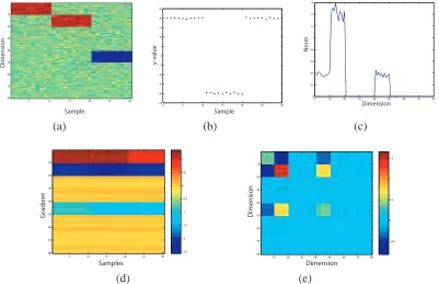
We construct a function in an n=80 dimensional space which consists of three linear functions over different partitions of the space. We generate 30 samples as follows:

1. For samples_{xi}10i=1

xj_∼

N

(1,σx), for j=1, . . . ,10; xj_∼

N

(0,σx), for j=11, . . . ,80.

2. For samples_{xi}20_i=11

xj∼

N

(1,σx),for j=11, . . . ,20; xj∼

N

(0,σx),for j=1, . . . ,10,21, . . . ,80.

3. For samples_{xi}30_i=21

xj_∼

N

(1,σx),for j=41, . . . ,50; xj_∼

N

(0,σx),for j=1, . . . ,40,51, . . . ,80.

A draw of this x matrix is shown in figure (1a). Three vectors with support over different dimensions were constructed as follows:

w1 = 2+.5 sin(2πi/10) for i=1, ...,10 and 0 otherwise, w2 = −2−.5 sin(2πi/10) for i=11, ...,20 and 0 otherwise, w3 = ₋2₋.5 sin(2πi/10) for i=41, ...,50 and 0 otherwise.

The values for_{yi}30_i=1were given by the following linear equations

1. For samples_{yi}10_i=1

yi=xi·w1+

N

(0,σy), 2. For samples_{yi}20_i=11

yi=xi·w2+

N

(0,σy), 3. For samples_{yi}30_i=21

yi=xi·w3+

N

(0,σy). A draw of the y values is shown in figure (1b).

In figure (1c) we plot the norm of each component of the estimate of the gradient,_{k(~fz,λ)ℓkK}80ℓ=1 forσx=.05 andσy=.30. The norm of each component gives an indication of the importance of a variable and variables with small norms can be eliminated. Note that the coordinates with nonzero norm are the ones we expect,ℓ=1, . . . ,20,41, . . . ,50.

5 10 15 20 25 30 10

20 30

40 50 60

70 80

Sample

Di

m

ens

ion

0 5 10 15 20 25 30 −25

−20 −15 −10 −5 0 5 10 15 20 25

y-v

alue

Sample

0 10 20 30 40 50 60 70 80 0

0.2 0.4 0.6 0.8 1 1.2 1.4 1.6

Dimension

No

rm

(a) (b) (c)

5 10 15 20 25 30 10

20

30

40

50

60

70

80 −2.5

−2 −1.5 −1 −0.5 0 0.5 1

Samples

Gr

a

dien

t

10 20 30 40 50 60 70 80 10

20

30

40

50

60

70

80

−0.5 0 0.5 1 1.5

Dimension

Di

m

ension

(d) (e)