Models of Cooperative Teaching and Learning
Sandra Zilles ZILLES@CS.UREGINA.CA
Department of Computer Science University of Regina
Regina, SK, Canada, S4S 0A2
Steffen Lange S.LANGE@FBI.H-DA.DE
Department of Computer Science
Darmstadt University of Applied Sciences Haardtring 100, 64295 Darmstadt, Germany
Robert Holte HOLTE@CS.UALBERTA.CA
Department of Computing Science University of Alberta
Edmonton, AB, Canada, T6G 2E8
Martin Zinkevich MAZ@YAHOO-INC.COM
Yahoo! Inc. 701 First Avenue
Sunnyvale, CA 94089, USA
Editor: Nicol`o Cesa-Bianchi
Abstract
While most supervised machine learning models assume that training examples are sampled at random or adversarially, this article is concerned with models of learning from a cooperative teacher that selects “helpful” training examples. The number of training examples a learner needs for identifying a concept in a given class C of possible target concepts (sample complexity of C) is lower in models assuming such teachers, that is, “helpful” examples can speed up the learning process.
The problem of how a teacher and a learner can cooperate in order to reduce the sample com-plexity, yet without using “coding tricks”, has been widely addressed. Nevertheless, the resulting teaching and learning protocols do not seem to make the teacher select intuitively “helpful” exam-ples. The two models introduced in this paper are built on what we call subset teaching sets and
recursive teaching sets. They extend previous models of teaching by letting both the teacher and
the learner exploit knowing that the partner is cooperative. For this purpose, we introduce a new notion of “coding trick”/“collusion”.
We show how both resulting sample complexity measures (the subset teaching dimension and the recursive teaching dimension) can be arbitrarily lower than the classic teaching dimension and known variants thereof, without using coding tricks. For instance, monomials can be taught with only two examples independent of the number of variables.
The subset teaching dimension turns out to be nonmonotonic with respect to subclasses of concept classes. We discuss why this nonmonotonicity might be inherent in many interesting co-operative teaching and learning scenarios.
1. Introduction
A central problem in machine learning is that learning algorithms often require large quantities of data. Data may be available only in limited quantity, putting successful deployment of stan-dard machine learning techniques beyond reach. This problem is addressed by models of machine learning that are enhanced by interaction between a learning algorithm (learner, for short) and its environment, whose main purpose is to reduce the amount of data needed for learning. Interaction here means that at least one party actively controls which information is exchanged about the target object to be learned. Most classic machine learning models address the “average case” of data pre-sentation to a learner (labeled examples are drawn independently at random from some distribution) or even the “worst case” (examples are drawn in an adversarial fashion). This results in the design of learners requiring more data than would be necessary under more optimistic (and often realistic) assumptions. As opposed to that, interactive learning refers to a “good case” in which representative examples are selected, whereby the number of examples needed for successful learning may shrink significantly.
Interactive machine learning is of high relevance for a variety of applications, for example, those in which a human interacts with and is observed by a learning system. A systematic and formally founded study of interactive learning is expected to result in algorithms that can reduce the cost of acquiring training data in real-world applications.
This paper focusses on particular formal models of interactive concept learning. Considering a finite instance space and a class of (thus finite) concepts over that space, it is obvious that each concept can be uniquely determined if enough examples are known. Much less obvious is how to minimize the number of examples required to identify a concept, and with this aim in mind models of cooperative learning and learning from good examples were designed and analyzed. The selection of good examples to be presented to a learner is often modeled using a teaching device (teacher) that is assumed to be benevolent by selecting examples expediting the learning process (see, for instance, Angluin and Krik¸is, 1997; Jackson and Tomkins, 1992; Goldman and Mathias, 1996; Mathias, 1997).
Throughout this paper we assume that teaching/learning proceeds in a simple protocol; the teacher presents a batch of labeled examples (that is, a set of instances, each paired with a label 1 or 0, according to whether or not the instance belongs to the target concept) to the learner and the learner returns a concept it believes to be the target concept. If the learner’s conjecture is correct, the exchange is considered successful. The sample size, that is, the number of examples the teacher presents to the learner, is the object of optimization; in particular we are concerned with the worst case sample size measured over all concepts in the underlying class C of all possible target concepts. Other than that, computational complexity issues are not the focus of this paper.
reader is referred to Angluin and Krik¸is (1997), Ott and Stephan (2002) and Goldman and Mathias (1996). It is often more convenient to define what constitutes a valid pair of teacher and learner.
The most popular teaching model is the one introduced by Goldman and Mathias (1996). Here a team of teacher and learner is considered valid if, for every concept c in the underlying class C the following properties hold.
• The teacher selects a set S of labeled examples consistent with c.
• On input of any superset of S of examples that are labeled consistently with c, the learner will return a hypothesis representing c.
The idea behind this definition is that the absence of examples in the sample S cannot be used for encoding knowledge about the target concept. This is completely in line with notions of inductive inference from good examples, see Freivalds et al. (1993) and Lange et al. (1998).
One way for a teacher and a learner to form a valid team under these constraints is for the teacher to select, for every concept c∈C, a sample S that is consistent with c but inconsistent with every other concept in C. The size of the minimum such sample is called the teaching dimension of c in C. The teaching dimension of the class C is the maximum teaching dimension over all concepts in C. For more information, the reader is referred to the original literature on teaching dimension and variants thereof (Shinohara and Miyano, 1991; Goldman and Kearns, 1995; Anthony et al., 1992).
The teaching dimension however does not always seem to capture the intuitive idea of coopera-tion in teaching and learning. Consider the following simple example. Let C0consist of the empty
concept and all singleton concepts over a given instance space X ={x1, . . . ,xn}. Each singleton concept{xi}has a teaching dimension of 1, since the single positive example(xi,+)is sufficient for determining{xi}. This matches our intuition that concepts in this class are easy to teach. In contrast to that, the empty concept has a teaching dimension of n—every example has to be pre-sented. However, if the learner assumed the teacher was cooperative—and would therefore present a positive example if the target concept was non-empty—the learner could confidently conjecture the empty concept upon seeing just one negative example.
Let us extend this reasoning to a slightly more complex example, the class of all boolean func-tions that can be represented as a monomial over m variables (m=4 in this example). Imagine yourself in the role of a learner knowing your teacher will present helpful examples. If the teacher sent you the examples
(0100,+),(0111,+),
what would be your conjecture? Presumably most people would conjecture the monomial M≡ v1∧v2, as does for instance the algorithm proposed by Valiant (1984). Note that this choice is not
uniquely determined by the data: the empty (always true) monomial and the monomials v1 and v2
are also consistent with these examples. And yet M seems the best choice, because we’d think the teacher would not have kept any bit in the two examples constant if it was not in the position of a relevant variable. In this example, the natural conjecture is the most specific concept consistent with the sample, but that does not, in general, capture the intuitive idea of cooperative learning. In particular, if, instead of the class of all monomials, the class of all complements of these concepts over the same instance space is chosen, then a cooperative teacher and learner would need only two negatively labeled example for teaching the complement of the concept associated with v1∧v2,
would change, but not the instances as such. The concepts guessed by the learner would then be neither the most specific nor the least specific concepts.
Could the learner’s reasoning about the teacher’s behavior in these examples be implemented without a coding trick? We will argue below that, for a very intuitive, yet mathematically rigorous definition of coding tricks, no coding trick is necessary to achieve exactly this behavior of teacher and learner; there are general strategies that teachers and learners can independently implement to cooperatively learn any finite concept class. When applied to the class of monomials this princi-ple enables any monomial to be learned from just two examprinci-ples, regardless of the number m of variables.
Our approach is to define a new model of cooperation in learning, based on the idea that each partner in the cooperation tries to reduce the sample size by exploiting the assumption that the other partner does so. If this idea is iteratively propagated by both partners, one can refine teaching sets iteratively ending up with a framework for highly efficient teaching and learning without any coding tricks. It is important to note that teacher and learner do not agree on any order of the concept class or any order of the instances. All they know about each others’ strategies is a general assumption about how cooperation should work independent of the concept class or its representation.
We show that the resulting variant of the teaching dimension—called the subset teaching di-mension (STD)—is not only a uniform lower bound of the teaching didi-mension but can be constant where the original teaching dimension is exponential, even in cases where only one iteration is needed. For example, as illustrated above, the STD of the class of monomials over m≥2 variables is 2, in contrast to its original teaching dimension of 2m.
Some examples however will reveal a nonmonotonicity of the subset teaching dimension: some classes possess subclasses with a higher subset teaching dimension, which is at first glance not very intuitive. We will explain below why in a cooperative model such a nonmonotonicity does not have to contradict intuition; additionally we introduce a second model of cooperative teaching and learning, that results in a monotonic dimension, called the recursive teaching dimension (RTD). Recursive teaching is based on the idea to let the teacher and the learner exploit a hierarchical structure that is intrinsic in the concept class. The canonical hierarchy associated with a concept class C is a nesting of C, starting with the class of all concepts in C that are easiest to teach (i.e., have the lowest teaching dimension) and then applying the nesting process recursively to the remaining set of concepts. At every stage, the recursive teaching sets for the concepts that are easiest to teach are the teaching sets for these concepts with respect to the class of remaining concepts. The recursive teaching dimension is the size of the largest recursive teaching set constructed this way.
The RTD-model is not as intuitive a model of cooperative teaching and learning as the STD-model is, but it displays a surprising set of properties. Besides its monotonicity, the RTD corre-sponds to teacher-learner protocols that do not violate Goldman and Mathias’s definition of teach-ing and learnteach-ing without codteach-ing tricks. Nevertheless, substantial improvements over the classical teaching dimension are obtained. A recent study furthermore shows that the recursive teaching dimension is a combinatorial parameter of importance when analyzing the complexity of learning problems from the perspective of active learning, teaching, learning from random examples, and sample compression, see Doliwa et al. (2010).
Both our teaching protocols significantly improve sample efficiency compared to previously studied variants of the teaching dimension.
2. Related Work
The problem of defining what are “good” or “helpful” examples in learning has been studied in several fields of learning theory.
Various learning models, which each involve one particular type of teacher, were proposed by Goldman and Kearns (1995), Goldman and Mathias (1996), Mathias (1997), Jackson and Tomkins (1992), Shinohara and Miyano (1991), Angluin and Krik¸is (1997), Angluin and Krik¸is (2003), Bal-bach (2008) and Kobayashi and Shinohara (2009); these studies mostly focus on learning boolean functions. See also Balbach and Zeugmann (2009) for a recent survey. The teaching dimension model, independently introduced by Goldman and Kearns (1991; 1995) and by Shinohara and Miyano (1991), is concerned with the sample complexity of teaching arbitrary consistent learn-ers. Samples that will allow any consistent learner to identify the target concept are called teaching sets; the maximum size of minimal teaching sets of all concepts in the underlying concept class C is called the teaching dimension of C. The problem of avoiding unfair “coding tricks” between teach-ers and learnteach-ers is addressed in particular by Goldman and Mathias (1996) with the introduction of a formal notion of collusion-free learning. It is known that computing (the size of) minimal teaching sets is in general intractable, see Servedio (2001), which is one reason why the polynomial-time models introduced by Jackson and Tomkins (1992) are of interest. Jackson and Tomkins no longer require that teachers choose samples that make any consistent learner successful; they rather focus on specific teacher/learner pairs. Loosening the requirement of learners being consistent, Kobayashi and Shinohara (2009) analyze how restrictions on the number of examples given by the teacher in-fluence the worst-case error of the hypothesis returned by a learner.
The teaching dimension was analyzed in the context of online learning, see Ben-David and Eiron (1998) and Rivest and Yin (1995), and in the model of learning from queries, for example, by Heged˝us (1995) and by Hanneke (2007), with a focus on active learning in the PAC framework. In contrast to these models, in inductive inference the learning process is not necessarily considered to be finite. Approaches to defining learning infinite concepts from good examples (Freivalds et al., 1993; Lange et al., 1998) do not focus on the size of a finite sample of good examples, but rather on characterizing the cases in which learners can identify concepts from only finitely many examples.
One of the two approaches we present in this paper is mainly based on an idea by Balbach (2008). He defined and analyzed a model in which, under the premise that the teacher uses a minimal teaching set (as defined by Goldman and Kearns, 1991, 1995) as a sample, a learner can reduce the size of a required sample by eliminating concepts which possess a teaching set smaller than the number of examples provided by the teacher so far. Iterating this idea, the size of the teaching sets might be gradually reduced significantly. Though our approach is syntactically quite similar to Balbach’s, the underlying idea is a different one (we do not consider elimination by the sample size but elimination by the sample content as compared to all possible teaching sets). The resulting variant of the teaching dimension in general yields different performance results in terms of sample size than Balbach’s model does.
3. The Teaching Dimension and the Balbach Teaching Dimension
In the models of teaching and learning to be defined below, we will always assume that the goal in an interaction between a teacher and a learner is to make the learner identify a (finite) concept over a (finite) instance space X .
Most of the recent work on teaching (cf. Balbach, 2008; Zilles et al., 2008; Balbach and Zeug-mann, 2009; Kobayashi and Shinohara, 2009) defines a concept simply as a subset of X and a concept class as a set of subsets of X . In effect, this is exactly the definition we would need for introducing the teaching models we define below. However, the definition and discussion of the notion of collusion (i.e., the conceptualization of what constitutes a coding trick), see Section 4, motivates a more general definition of concepts and concept classes. This more general definition considers the instance space X as an ordered set and every concept class C as an ordered set of subsets of X .
To formalize this, let X ={1, . . . ,n}. Concepts and concept classes are defined as follows.
Definition 1 Let z∈N.
A concept class of cardinality z is defined by an injective mapping C :{1, . . . ,z} →2[n]. Every i∈ {1, . . . ,z}and thus every concept C(i)is associated with a membership function on X={1, . . . ,n}, given by C(i)(j) = +if j∈C(i), and C(i)(j) =−if j∈/C(i), where 1≤j≤n. Thus a concept class C of cardinality z∈Nis represented as a matrix(C(i)(j))1≤i≤z,1≤j≤nover{+,−}.
C
zdenotes the collection of all concept classes of cardinality z.C
=Sz∈NC
zdenotes thecollec-tion of all concept classes (of any cardinality).
Consequently, concepts and concept classes considered below will always be finite.
Definition 2 Let z∈Nand C∈
C
z.A sample is a set S={(j1,l1), . . . ,(jr,lr)} ⊆X× {+,−}, where every element (j,l) of S is
called a (labeled) example.
Let i∈ {1, . . . ,z}. C(i)is consistent with S (and S is consistent with C(i)) if C(i)(jt) =lt for all
t∈ {1, . . . ,r}. Denote
Cons(S,C) ={i∈ {1, . . . ,z} |C(i)is consistent with S}.
The power set of{1, . . . ,n} × {+,−}, that is, the set of all samples, is denoted by
S
.3.1 Protocols for Teaching and Learning in General
In what follows, we assume that a teacher selects a sample for a given target concept and that a learner, given any sample S, always returns an index of a concept from the underlying concept class C. Formally, if z∈Nand(C(i)(j))1≤i≤z,1≤j≤nis a concept class in
C
z, a teacher for C is a function τ:{1, . . . ,z} →S
; a learner for C is a functionλ:S
→ {1, . . . ,z}.In order to constrain the definition of validity of a teacher/learner pair to a desired form of inter-action in a learning process, the notion of adversaries will be useful. Adversaries will be considered third parties with the option to modify a sample generated by a teacher before this sample is given to a learner. Formally, an adversary is a relation Ad⊆
S
3. Intuitively, if(τ(i),C(i),S)∈Ad for some i∈ {1, . . . ,z}and some teacher τfor C= (C(i)(j))1≤i≤z,1≤j≤n, then the adversary has the option to modify τ(i) to S and the learner communicating withτ will get S rather thanτ(i) as input. A special adversary is the so-called trivial adversary Ad∗, which satisfies(S1,S2,S)∈Ad∗if and onlyAll teaching and learning models introduced below will involve a very simple protocol between a teacher and a learner (and an adversary).
Definition 3 Let P be a mapping that maps every concept class C∈
C
to a pair P(C) = (τ,λ)where τis a teacher for C andλis a learner for C. P is called a protocol; given C∈C
, the pair P(C)is called a protocol for C.1. Let z∈Nand let C∈
C
zbe a concept class. Let AdCbe an adversary. P(C) = (τ,λ)is calledsuccessful for C with respect to AdCifλ(S) =i for all pairs(i,S)where i∈ {1, . . . ,z}, S∈
S
,and(τ(i),C(i),S)∈AdC.
2. Let
A
= (AdC)C∈C be a family of adversaries. P is called successful with respect toA
if, forall C∈
C
, P(C)is successful for C with respect to AdC.Protocols differ in the strategies according to which the teacher and the learner operate, that is, according to which the teacher selects a sample and according to which the learner selects a concept. In all protocols considered below, teachers always select consistent samples for every given target concept and learners, given any sample S, always return a concept consistent with S if such a concept exists in the underlying class C. Formally, all teachersτfor a concept class C∈
C
z will fulfill i∈Cons(τ(i),C)for all i∈ {1, . . . ,z}; all learnersλfor a class C will fulfillλ(S)∈Cons(S,C)for all S∈
S
with Cons(S,C)6=/0. Moreover, all the adversaries Ad we present below will have thefollowing property:
for any three samples S1,S2,S∈
S
, if(S1,S2,S)∈Ad then S1⊆S⊆S2.However, this does not mean that we consider other forms of teachers, learners, or adversaries illegitimate. They are just beyond the scope of this paper.
The goal in sample-efficient teaching and learning is to design protocols that, for every concept class C, are successful for C while reducing the (worst-case) size of the samples the teacher presents to the learner for any target concept in C. At the same time, by introducing adversaries, one tries to avoid certain forms of collusion, an issue that we will discuss in Section 4.
3.2 Protocols Using Minimal Teaching Sets and Balbach Teaching Sets
The fundamental model of teaching we consider here is based on the notion of minimal teaching sets, which is due to Goldman and Kearns (1995) and Shinohara and Miyano (1991).
Let z∈Nand let C∈
C
zbe a concept class. Let S be a sample. S is called a teaching set for i with respect to C if Cons(S,C) ={i}. A teaching set allows a learning algorithm to uniquely identify a concept in the concept class C. Teaching sets of minimal size are called minimal teaching sets. The teaching dimension of i in C is the size of such a minimal teaching set, that is, TD(i,C) =min{|S| |Cons(S,C) ={i}}, the worst case of which defines the teaching dimension of C, that is, TD(C) =max{TD(i,C)|1≤i≤z}. To refer to the set of all minimal teaching sets of i with respect to C, we use
TS(i,C) ={S|Cons(S,C) ={i}and|S|=TD(i,C)}.
Minimal teaching sets induce the following protocol.
Protocol 4 Let P be a protocol. P is called a teaching set protocol (TS-protocol for short) if the
1. τ(i)∈TS(i,C)for all i∈ {1, . . . ,z},
2. λ(S)∈Cons(S,C)for all S∈
S
with Cons(S,C)6= /0.This protocol is obviously successful with respect to the family consisting only of the trivial adversary. The teaching dimension of a concept class C is then a measure of the worst case sample size required in this protocol with respect to Ad∗when teaching/learning any concept in C.
The reason that, for every concept class C∈
C
z, the protocol P(C)is successful (with respect to Ad∗) is simply that a teaching set eliminates all but one concept due to inconsistency. However, if the learner knew TD(i,C)for every i∈ {1, . . . ,z}then sometimes concepts could also be eliminated by the mere number of examples presented to the learner. For instance, assume a learner knows that all but one concept C(i)have a teaching set of size one and that the teacher will teach using teaching sets. After having seen 2 examples, no matter what they are, the learner could eliminate all concepts but C(i). This idea, referred to as elimination by sample size, was introduced by Balbach (2008). If a teacher knew that a learner eliminates by consistency and by sample size then the teacher could consequently reduce the size of some teaching sets (e.g., here, if TD(i,C)≥3, a new “teaching set” for i could be built consisting of only 2 examples).More than that—this idea is iterated by Balbach (2008): if the learner knew that the teacher uses such reduced “teaching sets” then the learner could adapt his assumption on the size of the samples to be expected for each concept, which could in turn result in a further reduction of the “teaching sets” by the teacher and so on. The following definition captures this idea formally.
Definition 5 (Balbach, 2008)
Let z∈Nand let C∈
C
z be a concept class. Let i∈ {1, . . . ,z}and S a sample. Let BTD0(i,C) =TD(i,C). We define iterated dimensions for all k∈Nas follows.
• Conssize(S,C,k) ={i∈Cons(S,C)|BTDk(i,C)≥ |S|}.
• BTDk+1(i,C) =min{|S| |Conssize(S,C,k) ={i}}
Letκbe minimal such that BTDκ+1(i,C) =BTDκ(i,C)for all i∈ {1, . . . ,z}. The Balbach teaching dimension BTD(i,C)of i in C is defined by BTD(i,C) =BTDκ(i,C) and the Balbach teaching di-mension BTD(C)of the class C is BTD(C) =max{BTD(i,C)|1≤i≤z}.1 For every i∈ {1, . . . ,z}
we define
BTS(i,C) ={S|Conssize(S,C,κ) ={i}and|S|=BTD(i,C)}
and call every set in BTS(i,C)a minimal Balbach teaching set of i with respect to C. By Conssize(S,C)we denote the set Conssize(S,C,κ).
The Balbach teaching dimension measures the sample complexity of the following protocol with respect to the trivial adversary.
Protocol 6 Let P be a protocol. P is called a Balbach teaching set protocol (BTS-protocol for short)
if the following two properties hold for every C∈
C
, where P(C) = (τ,λ).1. τ(i)∈BTS(i,C)for all i∈ {1, . . . ,z},
2. λ(S)∈ {i|there is some S′∈BTS(i,C)such that S′⊆S}for all S∈
S
that contain a set S′∈ BTS(i,C)for some i∈ {1, . . . ,z}.Obviously, BTD(C)≤TD(C)for every concept class C∈
C
. How much the sample complexity can actually be reduced by a cooperative teacher/learner pair according to this “elimination by sample size” principle, is illustrated by the concept class C0 which consists of the empty conceptand all singleton concepts over X . The teaching dimension of this class is n, whereas the BTD is 2.
3.3 Teaching Monomials
A standard example of a class of boolean functions studied in learning theory is the class
F
m of monomials over a set{v1, . . . ,vm} of m variables, for any m≥2.2 Usually, this class is just de-fined by choosing X={0,1}m as the underlying instance space. Then, for any monomial M, the corresponding concept is defined as the set of those assignments in{0,1}mfor which M evaluates positively. Within our more general notion of concept classes, there is more than just one class of all monomials over m variables (which we will later consider as equivalent). This is due to distin-guishing different possible orderings over X and over the class of monomials itself.Definition 7 Let m∈N, m≥2 and assume n=2m, that is, X={1, . . . ,2m}.
Let bin :{1, . . . ,2m} → {0,1}m be a bijection, that is, a repetition-free enumeration of all bit
strings of length m. Let mon :{1, . . . ,3m} →
F
mbe a bijective enumeration of all monomial func-tions over m variables v1, . . . ,vm.A mapping C :{1, . . . ,3m} →2[2m] is called a concept class of all monomials over m variables if, for all i∈ {1, . . . ,3m}and all j∈ {1, . . . ,2m},
C(i)(j) =
(
+, if mon(i)evaluates to TRUE when assigning bin(j)to(v1, . . . ,vm),
−, if mon(i)evaluates to FALSE when assigning bin(j)to(v1, . . . ,vm).
It turns out that a class of all monomials contains only one concept for which the BTD-iteration yields an improvement.
Theorem 8 (Balbach, 2008) Let m∈N, m≥2. Let C :{1, . . . ,3m} →2[2m] be a concept class of all monomials over m variables. Let i∗∈ {1, . . . ,3m}with C(i∗) = /0be an index for the concept representing the contradictory monomial.
1. BTD(i∗,C) =m+2<2m=TD(i∗,C).
2. BTD(i,C) =TD(i,C)for all i∈ {1, . . . ,3m} \ {i∗}.
The intuitive reason for BTD(i∗,C) =m+2 in Theorem 8 is that samples for C(i∗)of size m+1 or smaller are consistent also with monomials different from C(i∗), namely those monomials that contain every variable exactly once (each such monomial is positive for exactly one of the 2m in-stances). These other monomials hence cannot be eliminated—neither by size nor by inconsistency.
4. Avoiding Coding Tricks
Intuitively, the trivial adversary of course does not prevent teacher and learner from using coding tricks. One way of defining what a coding trick is—or what a valid (collusion-free) behaviour of a teacher/learner is supposed to look like—is to require success with respect to a specific non-trivial type of adversary.
Goldman and Mathias (1996) called a pair of teacher and learner valid for a concept class C∈
C
z if, for every concept C(i)in the class C, the following properties hold.• The teacher selects a set S of labeled examples consistent with C(i).
• On input of any superset of S of examples that are labeled consistently with C(i), the learner will return a hypothesis representing C(i).
In other words, they considered a teacher-learner pair(τ,λ)a valid protocol for C if and only if it is successful with respect to any adversary AdCthat fulfillsτ(i)⊆S⊆C(i)for all i∈ {1, . . . ,z}and all S∈
S
with(τ(i),C(i),S)∈AdC.Obviously, teacher/learner pairs using minimal teaching sets according to the TS-protocol (Pro-tocol 4) are valid in this sense.
Theorem 9 Let z∈Nand let C∈
C
zbe a concept class. Letτbe a teacher for C,λa learner for C. If(τ,λ)is a TS-protocol for C then (τ,λ)is successful with respect to any adversary AdC thatfulfillsτ(i)⊆S⊆C(i)for all i∈ {1, . . . ,z}.
Proof. Immediate from the definitions.
Not only the protocol based on the teaching dimension (Protocol 4), but also the protocol based on the Balbach teaching dimension (Protocol 6) yields only valid teacher/learner pairs according to this definition—a consequence of Theorem 10.
Theorem 10 Let z∈N and let C∈
C
z be a concept class. Let i∈ {1, . . . ,z}, S∈BTS(i,C), andT⊇S such that i∈Cons(T,C). Then there is no i′∈Cons(T,C)such that i6=i′and S′⊆T for some S′∈BTS(i′,C).
Proof. Assume there is some i′ ∈Cons(T,C) such that i6=i′ and some S′ ∈BTS(i′,C) such that S′⊆T . Since both C(i)and C(i′)are consistent with T and both S and S′are subsets of T , we have i∈Cons(S′,C)and i′∈Cons(S,C). Now letκ≥1 be minimal such that BTDκ(i∗,C) =BTD(i∗,C)
for all i∗∈C. From i′∈Cons(S,C)and S∈BTS(i,C)we obtain
|S′|=BTDκ(i′,C)≤BTDκ−1(i′,C)<|S|.
Similarly, i∈Cons(S′,C)and S′∈BTS(i′,C)yields
|S|=BTDκ(i,C)≤BTDκ−1(i,C)<|S′|.
This is a contradiction.
Corollary 11 Let z∈Nand let C∈
C
zbe a concept class. Letτbe a teacher for C,λa learner for C. If(τ,λ)is a BTS-protocol for C then(τ,λ)is successful with respect to any adversary AdC thatfulfillsτ(i)⊆S⊆C(i)for all i∈ {1, . . . ,z}.
Goldman and Mathias’s definition of valid teacher/learner pairs encompasses a broad set of sce-narios. It accommodates all consistent learners even those that do not make any prior assumptions about the source of information (the teacher) beyond it being noise-free. However, in many appli-cation scenarios (e.g., whenever a human interacts with a computer or in robot-robot interaction) it is reasonable to assume that (almost) all the examples selected by the teacher are helpful or partic-ularly important for the target concept in the context of the underlying concept class. Processing a sample S selected by a teacher, a learner could exploit such an assumption by excluding not only all concepts that are inconsistent with S but also all concepts for which some examples in S would not seem particularly helpful/important. This would immediately call Goldman and Mathias’s definition of validity into question.
Here we propose a more relaxed definition of what a valid teacher/learner pair is (and thus, implicitly, a new definition of collusion). It is important to notice, first of all, that in parts of the existing literature, teaching sets and teaching dimension are defined via properties of sets rather than properties of representations of sets, see Balbach (2008) and Kobayashi and Shinohara (2009). Whenever this is the case, teacher/learner pairs cannot make use of the language they use for repre-senting instances in X or concepts in C. For example, teacher and learner cannot agree on an order over the instance space or over the concept class in order to encode information in samples just by the rank of their members with respect to the agreed-upon orders.
We want to make this an explicit part of the definition of collusion-free teacher/learner pairs. Intuitively, the complexity of teaching/learning concepts in a class should not depend on certain representational features, such as any order over X or over C itself. Moreover, negating the values of all concepts on a single instance should not affect the complexity of teaching and learning either. In other words, we want protocols to be “invariant” with respect to the following equivalence relation over
C
.Definition 12 Let z∈N. Let C= (C(i)(j))1≤i≤z,1≤j≤nand C′= (C′(i)(j))1≤i≤z,1≤j≤n be two
con-cept classes in
C
z. C and C′are called equivalent if there is a bijection frow:{1, . . . ,z} → {1, . . . ,z},a bijection fcol:{1, . . . ,n} → {1, . . . ,n}, and for every j∈ {1, . . . ,n} a bijection ℓj :{+,−} →
{+,−}, such that
C(i)(j) =ℓj(C′(frow(i))(fcol(j))for all i∈ {1, . . . ,z}, j∈ {1, . . . ,n}.
In this case,(frow,fcol,(ℓj)1≤j≤n)is said to witness that C and C′are equivalent.
We call a protocol collusion-free if it obeys this equivalence relation in the following sense.
Definition 13 Let P be a protocol. P is collusion-free if, for every z∈Nand C,C′∈
C
z, where C and C′ are equivalent as witnessed by(frow,fcol,(ℓj)1≤j≤n), the following two properties hold forP(C) = (τ,λ)and P(C′) = (τ′,λ′).
1. If 1≤i≤z andτ(i) ={(j1,l1), . . . ,(jr,lr)}, then τ′(f
2. If{(j1,l1), . . . ,(jr,lr)} ∈
S
andλ({(j1,l1), . . . ,(jr,lr)}) =i, then λ′({(fcol(j1), ℓj(l1)), . . . ,(fcol(jr), ℓj(lr))}) = frow(i).
It is obvious that both protocols introduced above are collusion-free.
Theorem 14 1. Every teaching set protocol is collusion-free.
2. Every Balbach teaching set protocol is collusion-free.
Proof. Immediate from the definitions.
The new protocols we define below are collusion-free as well. This means that all protocols studied in this article are defined independently of the order over X and C. Concept classes can hence be considered as sets of sets rather than matrices. Consequently, Definition 1 is more general than required in the rest of this paper. We therefore ease notation as follows.
X ={x1, . . . ,xn}denotes the instance space. A concept c is a subset of X and a concept class
C is a subset of the power set of X . We identify every concept c with its membership func-tion given by c(xi) = + if xi ∈c, and c(xi) =− if xi ∈/ c, where 1≤i≤n. Given a sample
S={(y1,l1), . . . ,(yr,lr)} ⊆X× {+,−}, we call c consistent with S if c(yi) =lifor all i∈ {1, . . . ,r}. If C is a concept class then Cons(S,C) ={c∈C|c is consistent with S}. S is called a teaching set for c with respect to C if Cons(S,C) ={c}. Then TD(c,C) =min{|S| |Cons(S,C) ={c}}, TD(C) =max{TD(c,C)|c∈C}, and TS(c,C) ={S|Cons(S,C) ={c}and|S|=TD(c,C)}. The notations concerning the Balbach teaching model are adapted by analogy.
5. The Subset Teaching Dimension
The approach studied by Balbach (2008) does not always meet the intuitive idea of teacher and learner exploiting the knowledge that either partner behaves cooperatively. Consider for instance one more time the class C0 containing the empty concept and all singletons over X={x1, . . . ,xn}. Each concept{xi}has the unique minimal teaching set{(xi,+)}in this class, whereas the empty concept only has a teaching set of size n, namely{(x1,−), . . . ,(xn,−)}. The idea of elimination by size allows a learner to conjecture the empty concept as soon as two examples have been provided, due to the fact that all other concepts possess a teaching set of size one. This is why the empty concept has a BTD equal to 2 in this example.
However, as we have argued in Section 1, it would also make sense to devise a learner in a way to conjecture the empty concept as soon as a first example for that concept is provided—knowing that the teacher would not use a negative example for any other concept in the class. In terms of teaching sets this means to reduce the teaching sets to their minimal subsets that are not contained in minimal teaching sets for other concepts in the given concept class.
In fact, a technicality in the definition of the Balbach teaching dimension (Definition 5) disal-lows the Balbach teaching dimension to be 1 unless the teaching dimension itself is already 1, as the following proposition states.
Proposition 15 Let C be a concept class. If BTD(C) =1 then TD(C) =1.
Since TD(C)>1, there exists a concept ˆc∈C such that TD(cˆ,C)>1. Since BTD(cˆ,C) =1, there exists a minimalκ≥1 such that BTDκ(cˆ,C) =BTD(cˆ,C) =1. In particular, there exists a sample S such that|S|=1 and
{c∈Cons(S,C)|BTDκ−1(c,C)≥1}={c}ˆ .
Since BTDκ−1(c,C)≥1 trivially holds for all c∈C, we obtain Cons(S,C) ={c}ˆ . Consequently, as |S|=1, it follows that TD(cˆ,C) =1. This contradicts the choice of ˆc. Thus TD(C) =1. So, if the Balbach model improves on the worst case teaching complexity, it does so only by improving the teaching dimension to a value of at least 2.
5.1 The Model
We formalize the idea of cooperative teaching and learning using subsets of teaching sets as follows.
Definition 16 Let C be a concept class, c ∈C, and S a sample. Let STD0(c,C) =TD(c,C), STS0(c,C) =TS(c,C). We define iterated sets for all k∈Nas follows.
• Conssub(S,C,k) ={c∈C|S⊆S′for some S′∈STSk(c,C)}.
• STDk+1(c,C) =min{|S| |Conssub(S,C,k) ={c}}
• STSk+1(c,C) ={S|Conssub(S,C,k) ={c},|S|=STDk+1(c,C)}.
Letκbe minimal such that STSκ+1(c,C) =STSκ(c,C)for all c∈C.3
A sample S such that Conssub(S,C,κ) ={c}is called a subset teaching set for c in C. The subset
teaching dimension STD(c,C) of c in C is defined by STD(c,C) =STDκ(c,C) and we denote by STS(c,C) =STSκ(c,C)the set of all minimal subset teaching sets for c in C. The subset teaching dimension STD(C)of C is defined by STD(C) =max{STD(c,C)|c∈C}.
For illustration, consider again the concept class C0, that is, C0={ci|0≤i≤n}, where c0= /0
and ci={xi}for all i∈ {1, . . . ,n}. Obviously, for k≥1,
STSk(ci) ={{(xi,+)}}for all i∈ {1, . . . ,n}
and
STSk(c0) ={{(xi,−)} |1≤i≤n}.
Hence STD(C0) =1 although TD(C0) =n.
Note that the example of the concept class C0establishes that the subset teaching dimension can
be 1 even if the teaching dimension is larger, in contrast to Proposition 15.
The definition of STS(c,C)induces a protocol for teaching and learning: For a target concept c, a teacher presents the examples in a subset teaching set for c to the learner. The learner will also be able to pre-compute all subset teaching sets for all concepts and determine the target concept from the sample provided by the teacher.4
3. Such aκexists because STD0(c,C)is finite and can hence be reduced only finitely often.
Protocol 17 Let P be a protocol. P is called a subset teaching set protocol (STS-protocol for short)
if the following two properties hold for every C⊆
C
, where P(C) = (τ,λ).1. τ(c)∈STS(c,C)for all c∈C,
2. λ(S)∈ {c|there is some S′ ∈STS(c,C)such that S′ ⊆S} for all S∈
S
that contain a set S′∈STS(c,C)for some c∈C.Note that Definition 16 does not presume any special order of the concept representations or of the instances, that is, teacher and learner do not have to agree on any such order to make use of the teaching and learning protocol. That means, given a special concept class C, the computation of its subset teaching sets does not involve any special coding trick depending on C—it just follows a general rule.
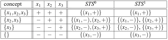
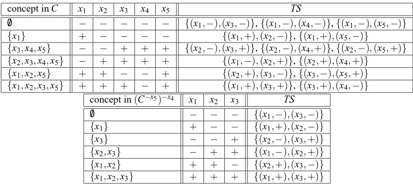
By definition, every subset teaching set protocol is collusion-free. However, teacher-learner pairs following a subset teaching set protocol are not necessarily valid in the sense of Goldman and Mathias’s definition. This is easily seen for the concept class Cθ of all linear threshold functions over three instances x1,x2,x3. This class has four concepts, namely c1={x1,x2,x3}, c2={x2,x3},
c3 ={x3}, and c4 ={}. It is easy to verify that {(x1,−)} is a subset teaching set for c2 and is
consistent with c3. Similarly, {(x3,+)} is a subset teaching set for c3 and is consistent with c2.
Hence{(x1,−),(x3,+)}is consistent with both c2and c3and contains a subset teaching set for c2
as well as a subset teaching set for c3. Obviously, there exists a teacher-learner pair(τ,λ)satisfying
the properties of an ST S−protocol for this class, such thatτ(c2) ={(x1,−)},τ(c3) ={(x3,+)}, and
λ({(x1,−),(x3,+)}) =c2. However, there is no learnerλ′such that(τ,λ′)is a valid teacher-learner
pair for Cθ. Such a learnerλ′ would have to hypothesize both c2and c3on input{(x1,−),(x3,+)}.
See Table 1 for illustration of this example.
concept x1 x2 x3 STS0 STS1
{x1,x2,x3} + + + {(x1,+)} {(x1,+)}
{x2,x3} − + + {(x1,−),(x2,+)} {(x1,−)},{(x2,+)}
{x3} − − + {(x2,−),(x3,+)} {(x2,−)},{(x3,+)}
{} − − − {(x3,−)} {(x3,−)}
Table 1: Iterated subset teaching sets for the class Cθ.
5.2 Comparison to the Balbach Teaching Dimension
Obviously, when using the trivial adversary, Protocol 17 based on the subset teaching dimension never requires a sample larger than a teaching set; often a smaller sample is sufficient. However, compared to the Balbach teaching dimension, the subset teaching dimension is superior in some cases and inferior in others. The latter may seem unintuitive, but is possible because Balbach’s teaching sets are not restricted to be subsets of the original teaching sets.
Theorem 18 1. For each u∈Nthere is a concept class C such that STD(C) =1 and BTD(C) = u.
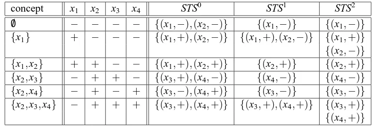
Proof. Assertion 1. Let n=2u+u be the number of instances in X . Define a concept class C=
Cupairas follows. For every s= (s1, . . . ,su)∈ {+,−}u, C contains the concepts cs,0={xi|1≤i≤
u and si= +}and cs,1=cs,0∪ {xu+1+int(s)}. Here int(s)∈Nis defined as the sum of all values 2u−i for which si= +, 1≤i≤u. We claim that STD(C) =1 and BTD(C) =u. See Table 2 for the case
u=2.
Let s= (s1, . . . ,su)∈ {+,−}u. Then
TS(cs,0,C) = {{(xi,si)|1≤i≤u} ∪ {(xu+1+int(s),−)}} and TS(cs,1,C) = {{(xu+1+int(s),+)}}
Since for each c∈C the minimal teaching set for c with respect to C contains an example that does not occur in the minimal teaching set for any other concept c′∈C, one obtains STD(C) =1 in just one iteration.
In contrast to that, we obtain
BTD0(cs,0,C) = u+1,
BTD1(cs,0,C) = u,
and BTD0(cs,1,C) = 1 for all s∈ {+,−}u.
Consider any s∈ {+,−}uand any sample S⊆ {(x,c
s,0(x))|x∈X}with|S|=u−1. Clearly there is
some s′∈ {+,−}uwith s′6=s such that c
s′,0∈Cons(S,C). So|Cons(S,C,+)|>1 and in particular Cons(S,C,+)6={cs,0}. Hence BTD2(cs,0,C) =BTD1(cs,0,C), which finally implies BTD(C) =u.
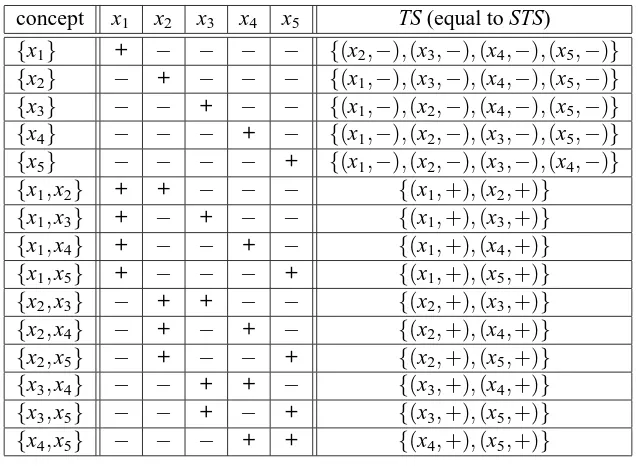
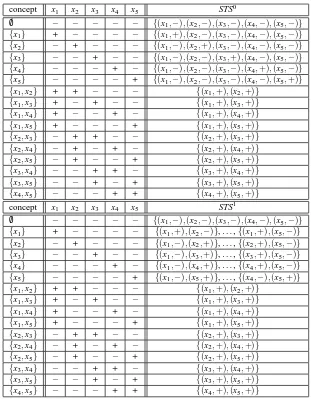
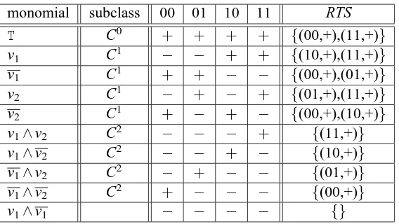
Assertion 2. Let n=u+1 be the number of instances in X . Define a concept class C=C1u/2as follows. For every i,j∈ {1, . . . ,u+1}, C contains the concept {xi}and the concept{xi,xj}. See Table 3 for the case u=4.
Then the only minimal teaching set for a singleton {xi} is the sample Si ={(x,−)|x6=xi} with|Si|=u. The only minimal teaching set for a concept{x
i,xj}with i6= j is the sample Si,j=
{(xi,+),(xj,+)}.
On the one hand, every subset of every minimal teaching set for a concept c∈C is contained in some minimal teaching set for some concept c′∈C with c6=c′. Thus STSk(c,C) =TS(c,C)for all c∈C and all k∈N. Hence STD(C) =TD(C) =u.
On the other hand, any sample S containing (xi,+) and two negative examples (xα,−) and
(xβ,−)(where i,α, andβare pairwise distinct) is in BTS({xi},C). This holds because every other concept in C that is consistent with this sample is a concept containing two instances and thus has a
teaching set of size smaller than 3 (=|S|). Thus BTD(C) =3.
5.3 Teaching Monomials
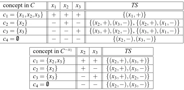
This section provides an analysis of the STD for a more natural example, the monomials, showing that the very intuitive example given in the introduction is indeed what a cooperative teacher and learner in an STS-protocol would do. The main result is that the STD of the class of all monomials is 2, independent on the number m of variables, whereas its teaching dimension is exponential in m and its BTD is linear in m, see Balbach (2008).
concept x1 x2 x3 x4 x5 x6 STS0 STS1
/0 [−] [−] [−] − − − {(x1,−),(x2,−),(x3,−)} {(x3,−)}
{x3} − − [+] − − − {(x3,+)} {(x3,+)}
{x2} [−] [+] − [−] − − {(x1,−),(x2,+),(x4,−)} {(x4,−)}
{x2,x4} − + − [+] − − {(x4,+)} {(x4,+)}
{x1} [+] [−] − − [−] − {(x1,+),(x2,−),(x5,−)} {(x5,−)}
{x1,x5} + − − − [+] − {(x5,+)} {(x5,+)}
{x1,x2} [+] [+] − − − [−] {(x1,+),(x2,+),(x6,−)} {(x6,−)}
{x1,x2,x6} + + − − − [+] {(x6,+)} {(x6,+)}
Table 2: Iterated subset teaching sets for the class Cu
pair with u = 2, where Cpairu =
{c−−,0,c−−,1. . . ,c++,0,c++,1} with c−−,0 = /0, c−−,1 ={x3}, c−+,0 ={x2}, c−+,1 =
{x2,x4}, c+−,0={x1}, c+−,1={x1,x5}, c++,0={x1,x2}, c++,1={x1,x2,x6}. All labels
contributing to minimal teaching sets are highlighted by square brackets.
concept x1 x2 x3 x4 x5 TS (equal to STS)
{x1} + − − − − {(x2,−),(x3,−),(x4,−),(x5,−)}
{x2} − + − − − {(x1,−),(x3,−),(x4,−),(x5,−)}
{x3} − − + − − {(x1,−),(x2,−),(x4,−),(x5,−)}
{x4} − − − + − {(x1,−),(x2,−),(x3,−),(x5,−)}
{x5} − − − − + {(x1,−),(x2,−),(x3,−),(x4,−)}
{x1,x2} + + − − − {(x1,+),(x2,+)}
{x1,x3} + − + − − {(x1,+),(x3,+)}
{x1,x4} + − − + − {(x1,+),(x4,+)}
{x1,x5} + − − − + {(x1,+),(x5,+)}
{x2,x3} − + + − − {(x2,+),(x3,+)}
{x2,x4} − + − + − {(x2,+),(x4,+)}
{x2,x5} − + − − + {(x2,+),(x5,+)}
{x3,x4} − − + + − {(x3,+),(x4,+)}
{x3,x5} − − + − + {(x3,+),(x5,+)}
{x4,x5} − − − + + {(x4,+),(x5,+)}
Table 3: Iterated subset teaching sets for the class C1u/2with u=4.
Proof. Let m∈N, m≥2 and s= (s1, . . . ,sm), s′= (s′
1, . . . ,s′m) elements in{0,1}m. Let∆(s,s′) denote the Hamming distance of s and s′, that is,∆(s,s′) =∑1≤i≤m|s(i)−s′(i)|.
We distinguish the following types of monomials M over m variables. Type 1: M is the empty monomial (i.e., the always true concept). Type 2: M involves m variables, M6≡v1∧v1.5
Type 3: M involves k variables, 1≤k<m, M6≡v1∧v1.
Type 4: M is contradictory, that is, M≡v1∧v1.
The following facts summarize some rather obvious properties of the corresponding minimal teaching sets for monomials (cf., for example Balbach, 2008, for more details).
Fact 1: Let M be of Type 1 and let s,s′∈ {0,1}msuch that∆(s,s′) =m. Then S={(s,+),(s′,+)}
forms a minimal teaching set for M, that is, S∈STS0(M,C).
Fact 2: Let M be of Type 2 and let s∈ {0,1}mbe the unique assignment for which M evaluates positively. Moreover, let s1, . . . ,sm∈ {0,1}m be the m unique assignments with∆(s,s1) =· · ·=
∆(s,sm) =1. Then S={(s,+),(s1,−), . . . ,(sm,−)}forms the one and only minimal teaching set for M, that is, S∈STS0(M,C). (Note that any two negative examples in S have Hamming distance 2.)
Fact 3: Let M be of Type 3 and let s ∈ {0,1}m be one assignment for which M evaluates positively. Moreover, let s′∈ {0,1}mbe the unique assignment with∆(s,s′) =m−k for which M
evaluates positively and let s1, . . . ,sk ∈ {0,1}m be the k unique assignments with∆(s,s1) =· · ·=
∆(s,sk) =1 for which M evaluates negatively. Then S={(s,+),(s′,+),(s1,−), . . . ,(sk,−)}forms
a minimal teaching set for M, that is, S∈STS0(M,C). (Note that any two negative examples in S have Hamming distance 2.)
Fact 4: Let M be of Type 4 and let S={(s,−)|s∈ {0,1}m}. Then S forms the one and only minimal teaching set for M, that is, S∈STS0(M,C).
After the first iteration the following facts can be observed.
Fact 1(a): Let M be of Type 1 and let S∈STS0(M,C). Then S∈STS1(M,C).
This is due to the observation that any singleton subset S′⊆S is a subset of a teaching set in STS0(M′,C)for some M′of Type 2.
Fact 2(a): Let M be of Type 2 and let S∈STS0(M,C). Then S∈STS1(M,C).
This is due to the observation that any proper subset S′ ⊂S is a subset of a teaching set in STS0(M′,C)for some M′ of Type 3, if S′contains one positive example, or for some M′of Type 4, otherwise.
Fact 3(a): Let M be of Type 3 and let s∈ {0,1}m be one assignment for which M evaluates positively. Moreover, let s′∈ {0,1}mbe the unique assignment with∆(s,s′) =m−k for which M
evaluates positively and let S={(s,+),(s′,+)}. Then S∈STS1(M,C).
This is due to the following observations: (i) S is not a subset of any teaching set S′in STS0(M′,C)
for some M′ of Type 1, since the two positive examples in S′ have Hamming distance m. (ii) S is obviously not a subset of any teaching set S′in STS0(M′,C)for some M′6≡M of Type 3. (iii) Any sufficiently small “different” subset S′ of some teaching set in STS0(M,C)—that is, S′ contains at most two examples, but not two positive examples—is a subset of any teaching set in STS0(M′,C)
for some M′of Type 2, if S′contains one positive example, or for some M′of Type 4, otherwise. Fact 4(a): Let M be of Type 4 and let s∈ {0,1}mbe any assignment. Moreover, let s′∈ {0,1}m be any assignment with∆(s,s′)=6 2 and let S={(s,−),(s′,−)}. Then S∈STS1(M,C).
This is due to the following observations: (i) S is not a subset of any teaching set S′in STS0(M′,C)
for some M′of Type 2 or of Type 3, since any two negative examples in S′have Hamming distance 2. (ii) Any sufficiently small “different” subset S′of the unique teaching set in STS0(M,C)—that is, S′ contains at most two negative examples, but two having Hamming distance 2—is a subset of a teaching set in STS0(M′,C)for some M′of Type 2.
After the second iteration the following facts can be observed.
Fact 1(b): Let M be of Type 1 and let S∈STS1(M,C). Then S∈STS2(M,C).
Fact 2(b): Let M be of Type 2 and let s∈ {0,1}m be the unique assignment for which M evaluates positively. Moreover, let s′ ∈ {0,1}m be any assignments with ∆(s,s′) =1 and let S=
{(s,+),(s′,−)}. Then S∈STS2(M,C).
This is due to the following observations: (i) S is not a subset of any teaching set S′in STS1(M′,C)
for some M′ of Type 1, of Type 3 or of Type 4, since none of these teaching sets contains one posi-tive and one negaposi-tive example. (ii) S is obviously not a subset of any teaching set S′in STS1(M′,C)
for some M′6≡M of Type 2. (iii) Any sufficiently small “different” subset S′ of a teaching set in STS1(M,C)—that is, S′contains at most two examples, but not a positive and a negative example— is a subset of a teaching set in STS1(M′,C) for some M′ of Type 3, if S′ contains one positive example, or for some M′6≡M of Type 2, otherwise.
Fact 3(b): Let M be of Type 3 and let S∈STS1(M,C). Then S∈STS2(M,C).
This is due to the observation that any singleton subset S′⊆S is a subset of a teaching set in STS1(M′,C)for some M′of Type 2.
Fact 4(b): Let M be of Type 4 and let S∈STS1(M,C). Then S∈STS2(M,C).
This is due to the observation that any singleton subset S′⊆S is a subset of a teaching set in STS1(M′,C)for some monomial M′of Type 2.
Note at this point that, for any monomial M of any type, we have STD2(M,C) =2.
Finally, it is easily seen that STD3(M,C) =STD2(M,C) =2 for all M∈C. For illustration of this proof in case m=2 see Table 4.
A further simple example showing that the STD can be constant as compared to an exponential teaching dimension, this time with an STD of 1, is the following.
Let C∨mDNF contain all boolean functions over m≥2 variables that can be represented by a 2-term DNF of the form v1∨M, where M is a monomial that contains, for each i with 2≤i≤m, either
the literal vior the literal vi. Moreover, Cm∨DNFcontains the boolean function that can be represented by the monomial M′≡v1.6
Theorem 20 Let m∈N, m≥2.
1. TD(C∨mDNF) =2m−1.
2. STD(C∨mDNF) =1.
Proof. Assertion 1. Let S be a sample that is consistent with M′. Assume that for some s∈ {0,1}m, the sample S does not contain the negative example (s,−). Obviously, there is a 2-term DNF D≡v1∨M such that D is consistent with S∪ {(s,+)}and D6≡M′. Hence S is not a teaching set
for M′. Since there are exactly 2m−12-term DNFs that represent pairwise distinct functions in C, a teaching set for M′must contain at least 2m−1examples.
Assertion 2. The proof is straightforward: Obviously, TD(D,C) =1 for all D∈C with D6≡M′. In particular, STD(D,C) =1 for all D∈C with D6≡M′. It remains to show that STD(M′,C) =1. For this it suffices to see that a minimal teaching set for M′ in C must contain negative examples, while no minimal teaching set for any D∈C with D6≡M′ contains any negative examples. Hence
STD2(M′,C) =1 and thus STD(M′,C) =1.
monomial 00 01 10 11 STS0 STS1 v1 − − + + {(10,+),(11,+),(00,-)} {(10,+),(11,+)}
{(10,+),(11,+),(01,-)}
v1 + + − − {(00,+),(01,+),(10,-)} {(00,+),(01,+)} {(00,+),(01,+),(11,-)}
v2 − + − + {(01,+),(11,+),(00,-)} {(01,+),(11,+)} {(01,+),(11,+),(10,-)}
v2 + − + − {(00,+),(10,+),(01,-)} {(00,+),(10,+)} {(00,+),(10,+),(11,-)}
v1∧v2 − − − + {(11,+),(01,-),(10,-)} {(11,+),(01,-),(10,-)}
v1∧v2 − − + − {(10,+),(00,-),(11,-)} {(10,+),(00,-),(11,-)}
v1∧v2 − + − − {(01,+),(00,-),(11,-)} {(01,+),(00,-),(11,-)}
v1∧v2 + − − − {(00,+),(01,-),(10,-)} {(00,+),(01,-),(10,-)}
v1∧v1 − − − − {(00,-),(01,-),(10,-),(11,-)} {(00,-),(01,-)} {(00,-),(10,-)} {(01,-),(11,-)} {(10,-),(11,-)}
T + + + + {(00,+),(11,+)} {(00,+),(11,+)} {(01,+),(10,+)} {(01,+),(10,+)}
monomial 00 01 10 11 STS2 STS3
v1 − − + + {(10,+),(11,+)} {(10,+),(11,+)}
v1 + + − − {(00,+),(01,+)} {(00,+),(01,+)}
v2 − + − + {(01,+),(11,+)} {(01,+),(11,+)}
v2 + − + − {(00,+),(10,+)} {(00,+),(10,+)}
v1∧v2 − − − + {(11,+),(01,-)} {(11,+),(01,-)} {(11,+),(10,-)} {(11,+),(10,-)}
v1∧v2 − − + − {(10,+),(00,-)} {(10,+),(00,-)} {(10,+),(11,-)} {(10,+),(11,-)}
v1∧v2 − + − − {(01,+),(00,-)} {(01,+),(00,-)} {(01,+),(11,-)} {(01,+),(11,-)}
v1∧v2 + − − − {(00,+),(01,-)} {(00,+),(01,-)} {(00,+),(10,-)} {(00,+),(10,-)}
v1∧v1 − − − − {(00,-),(01,-)} {(00,-),(01,-)} {(00,-),(10,-)} {(00,-),(10,-)} {(01,-),(11,-)} {(01,-),(11,-)} {(10,-),(11,-)} {(10,-),(11,-)}
T + + + + {(00,+),(11,+)} {(00,+),(11,+)} {(01,+),(10,+)} {(01,+),(10,+)}
6. Why Smaller Classes can be Harder to Teach
Interpreting the subset teaching dimension as a measure of complexity of a concept class in terms of cooperative teaching and learning, we observe a fact that is worth discussing, namely the non-monotonicity of this complexity notion, as stated by the following theorem.
Theorem 21 There is a concept class C such that STD(C′)>STD(C)for some subclass C′⊂C.
Proof. This is witnessed by the concept classes C=C1u/2∪ {/0}and its subclass C′=C1u/2used in the proof of Theorem 18.2, for any u>2 (see Table 3 and Table 5 for u=4). STD(C1u/2∪ {/0}) =2
while STD(Cu1/2) =u.
In contrast to that, it is not hard to show that BTD in fact is monotonic, see Theorem 22.
Theorem 22 If C is a concept class and C′⊆C a subclass of C, then BTD(C′)≤BTD(C).
Proof. Fix C and C′⊆C. We will prove by induction on k that
BTDk(c,C′)≤BTDk(c,C)for all c∈C′ (1)
for all k∈N.
k=0: Property (1) holds because of BTD0(c,C′) =TD(c,C′)≤TD(c,C) =BTD0(c,C)for all c∈C′.
Induction hypothesis: assume (1) holds for a fixed k. k k+1: First, observe that
Conssize(S,C′,k) = {c∈Cons(S,C′)|BTDk(c,C′)≥ |S|}
⊆ {c∈Cons(S,C′)|BTDk(c,C)≥ |S|}(ind. hyp.) ⊆ {c∈Cons(S,C)|BTDk(c,C)≥ |S|}
= Conssize(S,C,k)
Second, for all c∈C′we obtain
BTDk+1(c,C′) = min{|S| |Conssize(S,C′,k) ={c} }
≤ min{|S| |Conssize(S,C,k) ={c} }
≤ BTDk+1(c,C)
This completes the proof.
6.1 Nonmonotonicity After Elimination of Redundant Instances
Note that the nonmonotonicity of the subset teaching dimension holds with a fixed number of in-stances n. In fact, if n was not considered fixed then every concept class C′ would have a superset C (via addition of instances) of lower subset teaching dimension. However, the same even holds for the teaching dimension itself which we yet consider monotonic since it is monotonic given fixed n. So whenever we speak of monotonicity we assume a fixed instance space X .