Local Causal and Markov Blanket Induction for Causal Discovery
and Feature Selection for Classification
Part II: Analysis and Extensions
Constantin F. Aliferis [email protected]
Center of Health Informatics and Bioinformatics Department of Pathology
New York University New York, NY 10016, USA
Alexander Statnikov [email protected]
Center of Health Informatics and Bioinformatics Department of Medicine
New York University New York, NY 10016, USA
Ioannis Tsamardinos [email protected]
Computer Science Department, University of Crete
Institute of Computer Science, Foundation for Research and Technology, Hellas Heraklion, Crete, GR-714 09, Greece
Subramani Mani [email protected]
Discovery Systems Laboratory Department of Biomedical Informatics Vanderbilt University
Nashville, TN 37232, USA
Xenofon D. Koutsoukos [email protected]
Department of Electrical Engineering and Computer Science Vanderbilt University
Nashville, TN 37212, USA
Editor: Marina Meila
Abstract
to the state-of-the-art global learning algorithms. In addition, we investigate the use of non-causal feature selection methods to facilitate global learning. Open problems and future research paths related to local and local-to-global causal learning are discussed.
Keywords: local causal discovery, Markov blanket induction, feature selection, classification, causal structure learning, learning of Bayesian networks
1. Introduction
The present paper constitutes the second part of the study ofGeneralized Local Learning (GLL) which provides a unified framework for discovering local causal structure around a target variable of interest using observational data under broad assumptions. GLL supports local discovery of vari-ables that are direct causes or direct effects of the target and of the Markov blanket of the target. In the first part of the work (Aliferis et al., 2010) we introduced GLL and explained the importance of local causal discovery both for identification of highly predictive and parsimonious feature sets (feature selection problem), and for scaling up causal discovery. We then evaluated GLL instantia-tions against a plethora of state-of-the-art alternatives in many real, simulated and resimulated data sets. The main conclusions were that GLL algorithms achieved excellent predictivity, compactness and ability to learn local neighborhoods. Moreover, state-of-the-art non-causal feature selection methods often achieve excellent predictivity but are misleading in terms of causal discovery.
In the present paper we provide several extensions to GLL, study its properties, and extend to global graph learning using GLL as the core method. Because of the close relationship with Aliferis et al. (2010) we do not repeat here background material, technical definitions, or algorithm specifications. These are found in Aliferis et al. (2010), Sections 2-4.
2. Empirical Convergence and Comparison of Theoretical to Estimated Markov Blanket
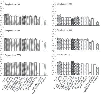
As explained in Aliferis et al. (2010), arguments about the suitability of Markov blanket induc-tion for feature selecinduc-tion for classificainduc-tion are based on large sample results, with convergence of small sample performance to the theoretical optimum being unknown. In the present section we use simulated data sets from published Bayesian networks to produce an empirical evaluation of classification performance convergence with respect to training sample size of two types of clas-sifiers: one that uses the estimated Markov blanket (MB(T)) or parents and children set (PC(T)) and one that uses the true MB(T)or PC(T)set (obtained from the known generative network). We use polynomial SVMs and KNN to fit each classifier type from three training sample sizes: 200, 500 and 5,000 samples. We note that GLL algorithms provide predictive and optimality guarantees for universal approximator classifiers and SVMs and KNN are used here as exemplars of this class of algorithms. In Aliferis et al. (2010) we also discuss more generally suitable classifiers, distribu-tions and loss funcdistribu-tions for GLL instantiadistribu-tions. An independent sample of 5,000 instances is used as evaluation test for classification performance (measured by AUC for binary and proportion of correct classifications for multiclass classification tasks). We use data sets sampled from 9 different Bayesian networks (See Table 15 in the Appendix). For each Bayesian network, we randomly se-lect 10 different targets and generate 5 samples (except for sample size 5,000 where one sample is generated) to reduce variability due to sampling.1 An independent sample of 5,000 instances is used as evaluation test for classification performance. Several local causal induction algorithms are used (including algorithms that induce direct causes/direct effects, and Markov blankets), and are com-pared to several non-causal algorithms to obtain reference points for baseline performance: RFE, UAF (univariate association filtering), L0, and LARS-EN (see Table 16 in the Appendix for the list of all algorithms). Classifier parameters (misclassification cost C and degree d for polynomial SVMs and number of neighbors K for KNN) are optimized by nested cross-validation following the same methodology as in Aliferis et al. (2010).
Results are presented in Figure 1 (and more details are given in Tables S19 and S20 of the online supplement). The main conclusions follow. Note that similar patterns are present when KNN is used instead of SVMs (with the only difference that convergence is slightly slower for KNN than for SVMs). For brevity we discuss here the SVM results only.
(a) Classification performance of the true parents and children and Markov blanket feature sets are not statistically significantly different at the 0.05 alpha level in sample 200 (p-value = 0.1440) and are statistically significantly different for larger samples (p-values = 0.0098 and
<0.0001 for sample sizes 500 and 5,000, respectively). The difference in SVM classification performance between using the PC(T)and MB(T)sets however does not exceed 0.02 AUC in favor of the MB(T)set. This means that even when the true PC(T) and MB(T)sets are known in the tested data, fitting classifiers from small data using the PC(T)set is as good as using the MB(T)set. In large sample, MB(T)features have a small predictive advantage over
PC(T)features.
0.5 0.55 0.6 0.65 0.7 0.75 0.8 0.85 0.9 0.95 1 0.5 0.55 0.6 0.65 0.7 0.75 0.8 0.85 0.9 0.95 1 True PC True MB HIT ON -PC (m
ax k =4)
HIT ON
-PC (m
ax k =3)
HIT ON
-PC (m
ax k =2)
HIT ON
-PC (m
ax k =1)
HIT ON
-MB ( max k=3 ) RFE (red uctio n by
50% )
RFE (red
uctio n by
20% ) UAF -KW -SVM (50% ) UAF -KW -SVM (20% ) UAF -S2N -SVM (50% ) UAF -S2N -SVM (20% ) L0 LAR S-EN (mul ticla ss) LAR S-E
N (o ne-v
ersu s-re
st)
All f eatu res 0.5 0.55 0.6 0.65 0.7 0.75 0.8 0.85 0.9 0.95 1
Sample size = 200
Sample size = 500
Sample size = 5000
N/A 0.5 0.55 0.6 0.65 0.7 0.75 0.8 0.85 0.9 0.95 1 0.5 0.55 0.6 0.65 0.7 0.75 0.8 0.85 0.9 0.95 1 0.5 0.55 0.6 0.65 0.7 0.75 0.8 0.85 0.9 0.95 1
Sample size = 200
Sample size = 500
Sample size = 5000
N/A True PC True MB HIT ON -PC (m
ax k =4) HIT ON -PC (max k=3 ) HIT ON -PC (m
ax k =2)
HIT ON
-PC (m
ax k =1)
HIT ON
-MB (m
ax k =3)
RFE (red
uctio n by
50% )
RFE (red
uctio n by
20% ) UA F-KW -SVM (50% ) UA F-K W-S VM (20% ) UA F-S2 N-S VM (50% ) UA F-S2 N-S VM (20% ) L0 LAR S-E
N (m ultic
lass )
LAR S-E
N (o ne-v
ersu s-re
st)
All f eatu
res
Figure 1: Classification performance of polynomial SVM (left) and KNN (right) classifiers in 9 simulated and resimulated data sets. Results are given for training sample sizes = 200, 500, and 5000. “True-PC” and “True-MB” correspond to the true PC(T) and MB(T)
feature sets obtained from the known generative network. The bars denote maximum and minimum performance over multiple training samples of each size (data is available only for sample sizes 200 and 500). The performances reported in the figure are averaged over all data sets, selected targets, and multiple samples of each size. L0 did not terminate within the allotted time limit for sample size 5000.
(c) The true PC(T)or true MB(T)features set when fitted from sample size of 200 has a small (0.02-0.03 AUC/proportion of correct classifications for SVM) advantage over the estimated
PC(T) or MB(T) features fitted from small sample. This difference is statistically signif-icant at the 0.05 alpha level with p-values 0.0144 and <0.0001 for the PC(T) and MB(T)
classifiers, respectively. Very quickly (as sample size becomes 500), this advantage becomes insignificant (0.01 point of AUC/proportion of correct classifications for SVM) with corre-sponding p-values 0.4708 and 0.0506 for the PC(T)and MB(T)classifiers, respectively. This implies that predictivity of estimated MB(T)and PC(T)sets converge to the optimal one very quickly with respect to sample size.
(d) Classifiers for estimated MB(T)/PC(T)sets fitted from small sample and classifiers for the true MB(T)/PC(T)sets fitted from small sample have indistinguishable performance in sam-ple size 500 (as shown in (c) above); then performance increases in samsam-ple size 5,000 for both types of classifiers (p-values ranging from<0.0001 to 0.0174 with AUC increases between 0.01 and 0.04). We thus conclude that fitting the right classifier parameters to the identified features is less sample efficient than identifying the right feature set.
(e) Some of the non-causal feature selection methods (e.g., L0, LARS-EN) tend to compare less favorably in small sample to their large sample performance compared to GLL algorithms.
3. Multiple Statistical Tests and Insensitivity to Irrelevant Variables
In this section we focus our attention to a subtle but an important problem facing many feature and causal discovery algorithms operating in very high dimensional spaces, namely the problem of mul-tiple statistical comparisons, which is exacerbated when many irrelevant features are present. We will show that GLL algorithms have inherent control to false positives due to multiple comparisons while the same is not true for other non-causal feature selection methods tested.
Briefly stated, when conducting n statistical tests with an error type I levelα(i.e., statistical sig-nificance level, that is probability that a truly null hypothesis is rejected, thus falsely concluding that a statistical difference or association or dependence exists when in reality it does not) it is expected thatα·n false positives will occur on average. Consider a common analysis situation in
bioinformat-ics research where a researcher conducts one test per variable (i.e., single nucleotide polymorphism (SNP)) in an assay with 10,000 SNP probes in total. 10,000 such tests need be conducted to see whether univariately each SNP probe is differentially present in two or more phenotype categories. If the researcher usesαequal to 5%, then under the null hypothesis (i.e., all 10,000 SNPs are not truly differentially expressed) the analysis will yield 500 false positive SNP probes. Standard statis-tical practice involves addressing the problem via one of two basic approaches. The first approach, the classic Bonferroni correction (Casella and Berger, 2002), adjusts theαby replacing it byα/n so
that in our example the 5% false positive rate is preserved for each feature selected by the multiple tests. This approach preserves the desiredα, but reduces the power to detect statistically significant features (namely the features that are truly differentially expressed and detectable at α but non-detectable at α/n), hence creates false negatives that were not present before the correction. The
Lung_Cancer
Sample size 0 1 2 3 4 0 1 2 3 4 0 1 2 3 4 0 1 2 3 4
100 1.00 0.99 0.99 0.99 0.99 0.97 0.99 0.98 0.98 0.98 0.63 0.63 0.62 0.62 0.62 0.50 0.50 0.50 0.50 0.50 200 1.00 1.00 0.99 0.98 0.98 0.99 1.00 0.99 0.99 0.99 0.67 0.69 0.67 0.66 0.66 0.51 0.50 0.49 0.50 0.50 500 1.00 1.00 1.00 1.00 1.00 1.00 1.00 1.00 1.00 1.00 0.67 0.72 0.73 0.72 0.71 0.50 0.50 0.51 0.49 0.49 1000 1.00 1.00 1.00 1.00 1.00 1.00 1.00 1.00 1.00 1.00 0.68 0.74 0.73 0.74 0.72 0.50 0.52 0.51 0.50 0.49 2000 1.00 1.00 1.00 1.00 1.00 1.00 1.00 1.00 1.00 1.00 0.69 0.74 0.74 0.74 0.74 0.49 0.50 0.49 0.50 0.49 5000 1.00 1.00 1.00 1.00 1.00 1.00 1.00 1.00 1.00 1.00 0.72 0.74 0.74 0.74 0.74 0.51 0.51 0.49 0.49 0.49
Alarm10
Sample size 0 1 2 3 4 0 1 2 3 4 0 1 2 3 4 0 1 2 3 4
100 0.95 0.95 0.95 0.95 0.95 0.83 0.92 0.92 0.92 0.92 0.66 0.69 0.69 0.69 0.69 0.50 0.50 0.50 0.50 0.50 200 0.96 0.95 0.95 0.95 0.95 0.89 0.95 0.95 0.95 0.95 0.68 0.77 0.78 0.78 0.78 0.50 0.50 0.50 0.50 0.50 500 0.96 0.96 0.96 0.96 0.96 0.93 0.95 0.95 0.95 0.95 0.71 0.80 0.80 0.80 0.81 0.50 0.51 0.50 0.50 0.50 1000 0.97 0.97 0.97 0.97 0.97 0.94 0.97 0.96 0.96 0.96 0.73 0.82 0.81 0.82 0.82 0.50 0.50 0.50 0.50 0.50 2000 0.97 0.97 0.97 0.97 0.97 0.96 0.97 0.97 0.97 0.97 0.76 0.82 0.82 0.82 0.82 0.50 0.50 0.50 0.50 0.50 5000 0.97 0.98 0.97 0.97 0.97 0.97 0.98 0.97 0.97 0.97 0.81 0.83 0.83 0.83 0.83 0.50 0.50 0.50 0.50 0.50
Version 1
(original network)
Version 2
(original network + irrelevant variables)
Version 3
(weakened signal + irrelevant variables)
Version 4
(only irrelevant variables)
max-k parameter
Version 1
(original network)
max-k parameter
Version 2
(original network + irrelevant variables)
Version 3
(weakened signal + irrelevant variables)
Version 4
(only irrelevant variables)
Low classification performance High classification performance
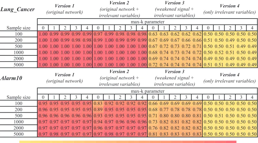
Table 1: Classification performance (AUC) of polynomial SVM estimated on 5,000 sample independent testing set for features selected by HITON-PC with parameter
max-k={0,1,2,3,4}on different training sample sizes{100,200,500,1000,2000,5000}. The color of each table cell denotes strength of predictivity with yellow (light) corresponding to low classification performance and red (dark) to high classification performance.
positives on average. In our example, FDR methods may, for example, allow the researcher to en-sure that on average no more than 10 out of 100 SNPs selected are false positives. This is highly useful in exploratory analysis of high-dimensional data where subsequent experimentation can sort out false positives easily but where false negatives have high cost.
Constraint-based causal methods employ, in large data sets and depending on connectivity and inclusion heuristic efficiency, many thousands of statistical tests of independence and are thus ex-pected a priori to be particularly sensitive to the multiple testing problem. We note that, rather not obviously at first, testing under the null hypothesis does not only occur when irrelevant features ex-ist but also whenever we test weakly relevant features conditioned on a set of variables that blocks all paths connecting it with the target. Other feature selection methods do not explicitly conduct sta-tistical tests of independence but may also be sensitive to many irrelevant features as we will show. In the present section we first systematically explore empirically and then examine theoretically the degree of sensitivity of GLL algorithms to irrelevant features, how they address the multiple test-ing problem, and how other feature selection and causal discovery algorithms compare along these dimensions.
In the first set of experiments we run only semi-interleaved HITON-PC without symmetry cor-rection on two networks and variants. The networks, described in Aliferis et al. (2010), are the
Lung_Cancer
Sample size 0 1 2 3 4 0 1 2 3 4 0 1 2 3 4
100 3.30 15.30 18.20 18.20 18.20 3.30 15.40 18.40 18.40 18.40 9.40 21.90 23.40 23.40 23.40 200 1.20 7.70 17.70 19.60 19.60 1.20 7.70 17.70 19.60 19.60 4.40 17.50 23.20 23.40 23.40 500 0.80 1.30 5.70 15.10 18.00 0.80 1.30 5.70 15.10 18.00 1.00 4.60 17.50 21.70 21.90 1000 0.30 1.00 1.50 5.40 11.70 0.30 1.00 1.50 5.40 11.70 0.80 1.70 6.60 17.50 19.90 2000 0.30 0.90 1.00 1.80 4.10 0.30 0.90 1.00 1.80 4.10 0.70 1.00 1.80 8.70 15.80 5000 0.00 0.40 1.00 1.10 1.10 0.00 0.40 1.00 1.10 1.10 0.30 0.80 1.00 1.40 4.80
Alarm10
Sample size 0 1 2 3 4 0 1 2 3 4 0 1 2 3 4
100 1.70 4.10 4.10 4.10 4.10 1.70 4.10 4.20 4.20 4.20 2.20 5.00 5.00 5.00 5.00 200 1.40 3.90 4.00 4.00 4.00 1.40 3.90 4.00 4.00 4.00 1.80 4.50 4.70 4.70 4.70 500 0.40 2.60 2.70 2.70 2.70 0.40 2.60 2.90 3.00 3.00 0.60 3.90 4.40 4.40 4.40 1000 0.10 2.00 2.10 2.10 2.10 0.10 2.00 2.20 2.20 2.20 0.80 3.60 3.90 4.00 4.00 2000 0.00 1.40 1.50 1.50 1.50 0.00 1.40 1.50 1.50 1.50 0.10 3.10 3.60 3.50 3.50 5000 0.00 0.50 1.10 1.20 1.20 0.00 0.50 1.10 1.20 1.20 0.00 1.40 1.70 1.80 1.80
Version 1 (original network)
Version 2 (original network + irrelevant
variables)
Version 3
(weakened signal + irrelevant variables)
max-k parameter
Version 1 (original network)
Version 2 (original network + irrelevant
variables)
Version 3
(weakened signal + irrelevant variables)
max-k parameter
Small number of false negatives Large number of false negatives
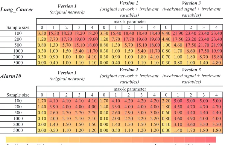
Table 2: Number of false negatives in the parents and children set for features selected by HITON-PC with parameter max-k={0,1,2,3,4} on different training sample sizes
{100,200,500,1000,2000,5000}. For Version 4 of the network the parents and children set is empty since there are no relevant variables. The color of each table cell denotes num-ber of false negatives with yellow (light) corresponding to smaller values and red (dark) to larger ones.
connectivity whereas the latter is designed to have lower connectivity. In the Lung Cancer network we focused our attention on the natural target variable; this target has 26 members of the parents and children set and 18 spouses, 14 irrelevant variables, and 741 weakly relevant ones. We created four versions of this network: Version 1 contains the original network (total number of variables 800). In Version 2 we augment the original network with 7990 irrelevant variables (total number of variables 8790). Version 3 is the same as Version 2, except for 10% of values of the target are ran-domly flipped to weaken the signal (total number of variables 8790). Finally, Version 4 is same as Version 2, except that there are only irrelevant variables and the target (total number of variables is 8790−741−18−26=8005). The tiled Alarm10 has also four corresponding versions but its target was chosen randomly and it has only 6 members of the parents and children set and no spouses. In both networks (and their variants) we create irrelevant variables by randomly permuting values of weakly and strongly variables so that the distribution of each variable values is realistic. With these 8 data set versions we can systematically examine the effects of presence of irrelevant variables, strength of predictive signal of features for the target, network connectivity and of the values of the GLL max-k parameter (Aliferis et al., 2010).
Lung_Cancer
Sample size 0 1 2 3 4 0 1 2 3 4 0 1 2 3 4
100 65.00 0.80 0.30 0.30 0.30 65.00 0.70 0.40 0.40 0.40 62.40 0.90 0.50 0.50 0.50 200 120.50 3.00 0.10 0.00 0.00 120.50 3.00 0.10 0.00 0.00 85.60 2.90 0.60 0.60 0.60 500 149.00 5.80 0.00 0.10 0.00 149.00 5.80 0.00 0.10 0.00 110.70 4.20 0.40 0.30 0.30 1000 202.90 11.60 0.10 0.00 0.00 202.90 11.60 0.10 0.00 0.00 123.70 5.70 0.00 0.00 0.00 2000 236.10 16.40 0.50 0.10 0.00 236.10 16.40 0.50 0.10 0.00 171.10 12.00 0.40 0.00 0.00 5000 410.40 30.80 2.60 0.10 0.00 410.40 30.80 2.60 0.10 0.00 272.60 20.30 1.10 0.00 0.00
Alarm10
Sample size 0 1 2 3 4 0 1 2 3 4 0 1 2 3 4
100 22.10 3.70 3.70 3.70 3.70 22.10 2.40 2.40 2.40 2.40 22.50 1.80 1.80 1.80 1.80 200 26.50 0.80 0.80 0.80 0.80 26.50 0.60 0.50 0.50 0.50 25.20 1.30 0.90 0.90 0.90 500 32.20 0.90 0.10 0.10 0.10 32.20 0.80 0.10 0.10 0.10 32.00 1.00 0.20 0.20 0.20 1000 30.20 1.40 0.00 0.00 0.00 30.20 1.30 0.00 0.00 0.00 27.10 0.70 0.10 0.30 0.30 2000 33.50 2.90 0.30 0.30 0.30 33.50 2.80 0.30 0.30 0.30 32.40 1.80 0.60 0.20 0.20 5000 38.00 5.40 0.30 0.20 0.10 38.00 5.30 0.30 0.20 0.10 37.30 3.10 0.20 0.20 0.20
Version 1 (original network)
Version 2 (original network + irrelevant variables)
Version 3 (weakened signal + irrelevant variables) max-k parameter
Version 1 (original network)
Version 2 (original network + irrelevant variables)
Version 3 (weakened signal + irrelevant variables) max-k parameter
Small number of false positives Large number of false positives
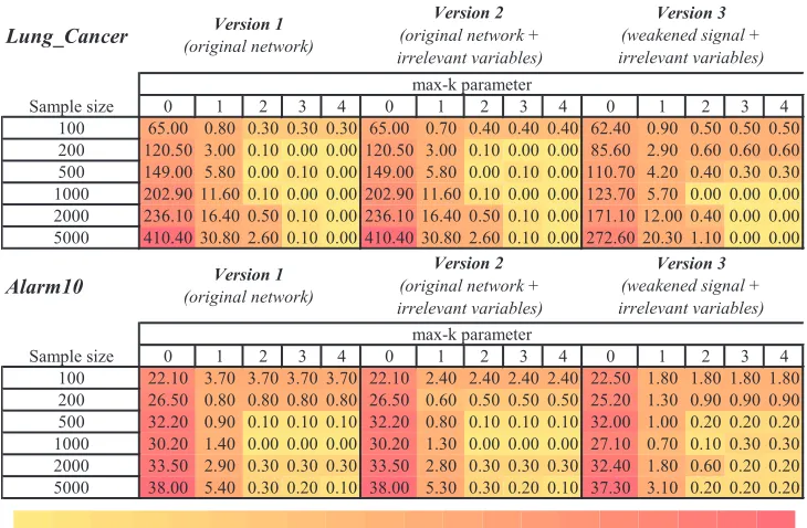
Table 3: Number of false positives (within weakly relevant variables) in the parents and children set for features selected by HITON-PC with parameter max-k={0,1,2,3,4}on different training sample sizes{100,200,500,1000,2000,5000}. For Version 4 of the network there are no weakly relevant variables. The color of each table cell denotes number of false positives with yellow (light) corresponding to smaller values and red (dark) to larger ones.
false positives that are irrelevant and total false positives. To ensure that our results are not affected by variability in small samples, we generate 10 random samples of each size and average results.
Tables 1– 5 provide evidence for the following conclusions:
(a) Classification performance is mildly or not affected by false positives and false negatives (Table 1). When many false negatives are present, predictivity is compensated by the few remaining strong relevant features plus strongly predictive weakly relevant ones. This im-plies that classification performance cannot be used to inform us about the presence of false positives/negatives.
(b) As expected, false negatives are reduced as sample size grows (because power increases), however they also increase as max-k grows, because the number of tests increases as max-k grows and thus overall power decreases (Table 2).
Lung_Cancer
Sample size 0 1 2 3 4 0 1 2 3 4 0 1 2 3 4 0 1 2 3 4
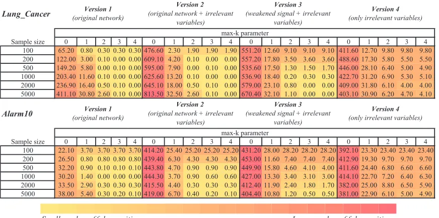
100 65.20 0.80 0.30 0.30 0.30 476.60 2.30 1.90 1.90 1.90 551.20 12.60 9.10 9.10 9.10 411.60 12.70 9.80 9.80 9.80 200 122.00 3.00 0.10 0.00 0.00 609.10 4.20 0.10 0.00 0.00 557.20 17.80 3.50 3.60 3.60 488.60 17.30 5.80 5.50 5.50 500 149.20 5.80 0.00 0.10 0.00 595.00 7.90 0.00 0.10 0.00 535.60 17.50 1.30 1.50 1.70 446.00 28.10 6.40 5.00 4.90 1000 203.40 11.60 0.10 0.00 0.00 625.60 13.20 0.10 0.00 0.00 536.90 18.40 0.20 0.30 0.30 422.70 31.20 6.90 5.30 5.10 2000 236.90 16.40 0.50 0.10 0.00 645.10 18.00 0.50 0.10 0.00 579.00 23.10 0.80 0.00 0.00 409.00 31.80 6.10 4.00 4.00 5000 411.10 30.80 2.60 0.10 0.00 813.50 32.50 2.60 0.10 0.00 670.40 32.10 1.10 0.00 0.00 403.10 30.90 6.20 4.70 4.10
Alarm10
Sample size 0 1 2 3 4 0 1 2 3 4 0 1 2 3 4 0 1 2 3 4
100 22.10 3.70 3.70 3.70 3.70 414.20 25.40 25.20 25.20 25.20 431.20 28.00 28.20 28.20 28.20 392.10 23.30 23.40 23.40 23.40 200 26.50 0.80 0.80 0.80 0.80 439.40 6.30 4.30 4.30 4.30 453.00 11.60 7.40 7.40 7.40 412.90 19.30 9.70 9.70 9.70 500 32.20 0.90 0.10 0.10 0.10 443.80 4.70 0.90 0.90 0.90 449.90 15.80 4.60 4.10 4.00 411.60 24.40 6.80 6.60 6.60 1000 30.20 1.40 0.00 0.00 0.00 444.30 3.70 0.90 0.60 0.60 427.00 13.30 3.40 3.10 3.00 414.10 22.70 7.20 6.40 6.30 2000 33.50 2.90 0.30 0.30 0.30 415.50 4.40 0.30 0.30 0.30 412.40 11.90 2.40 1.80 1.70 382.00 25.00 8.80 6.50 5.90 5000 38.00 5.40 0.30 0.20 0.10 419.00 6.70 0.40 0.20 0.10 404.40 10.80 1.20 0.50 0.50 381.00 22.90 6.10 5.00 4.90
max-k parameter
Version 1
(original network)
Version 2
(original network + irrelevant variables)
Version 3
(weakened signal + irrelevant variables)
Version 4
(only irrelevant variables)
max-k parameter
Version 1
(original network)
Version 2
(original network + irrelevant variables)
Version 3
(weakened signal + irrelevant variables)
Version 4
(only irrelevant variables)
Small number of false positives Large number of false positives
Table 4: Number of false positives in the parents and children set for features selected by HITON-PC with parameter max-k={0,1,2,3,4} on different training sample sizes
{100,200,500,1000,2000,5000}. The color of each table cell denotes number of false positives with yellow (light) corresponding to smaller values and red (dark) to larger ones.
sample size and sufficient (but not excessive) max-k, (i.e., sample size ≥2,000, max-k=2) (Tables 2 and 4).
(d) When irrelevant features are present, as sample size grows the number of false positives that are weakly relevant increases if max-k is not sufficient to block paths from/to each weakly relevant to/from the target. As max-k increases, the false positives decrease to the point that they vanish (Table 3). False positives due to irrelevant features (Table 5) quickly vanish as
max-k becomes 2 or higher and this holds as long as sample size is larger than 200. False
negatives are not affected by presence of irrelevant features (Table 2). Thus, overall, with enough sample size and right value of max-k, both false negatives and false positives vanish (Tables 2 and 4).
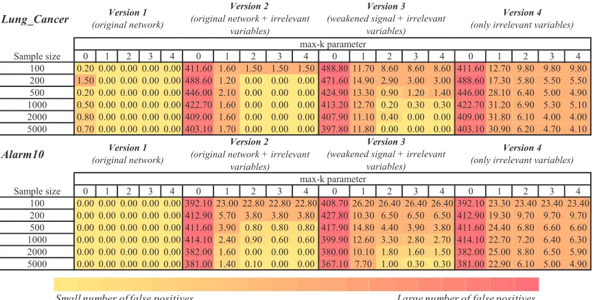
(e) When the predictive signal is weaker, both false negatives are increased and false positives within weakly relevant variables are decreased for a given sample size (because power is smaller) (Tables 2 and 3). However false positive irrelevant variables (Table 5) are increased. This is due to the fact that fewer features enter the TPC(T) set thus leading to fewer tests that can be performed hence smaller capacity to remove irrelevant false positives. As previ-ously with enough sample and right max-k, false positives and negatives are fully eliminated (Tables 2 and 4).
(f) When the data consists only of irrelevant features, false positives (irrelevant) are reduced as
max-k increases for all sample sizes (Table 5). There is a very small persistent residual number
phenom-Lung_Cancer
Sample size 0 1 2 3 4 0 1 2 3 4 0 1 2 3 4 0 1 2 3 4
100 0.20 0.00 0.00 0.00 0.00 411.60 1.60 1.50 1.50 1.50 488.80 11.70 8.60 8.60 8.60 411.60 12.70 9.80 9.80 9.80 200 1.50 0.00 0.00 0.00 0.00 488.60 1.20 0.00 0.00 0.00 471.60 14.90 2.90 3.00 3.00 488.60 17.30 5.80 5.50 5.50 500 0.20 0.00 0.00 0.00 0.00 446.00 2.10 0.00 0.00 0.00 424.90 13.30 0.90 1.20 1.40 446.00 28.10 6.40 5.00 4.90 1000 0.50 0.00 0.00 0.00 0.00 422.70 1.60 0.00 0.00 0.00 413.20 12.70 0.20 0.30 0.30 422.70 31.20 6.90 5.30 5.10 2000 0.80 0.00 0.00 0.00 0.00 409.00 1.60 0.00 0.00 0.00 407.90 11.10 0.40 0.00 0.00 409.00 31.80 6.10 4.00 4.00 5000 0.70 0.00 0.00 0.00 0.00 403.10 1.70 0.00 0.00 0.00 397.80 11.80 0.00 0.00 0.00 403.10 30.90 6.20 4.70 4.10
Alarm10
Sample size 0 1 2 3 4 0 1 2 3 4 0 1 2 3 4 0 1 2 3 4
100 0.00 0.00 0.00 0.00 0.00 392.10 23.00 22.80 22.80 22.80 408.70 26.20 26.40 26.40 26.40 392.10 23.30 23.40 23.40 23.40 200 0.00 0.00 0.00 0.00 0.00 412.90 5.70 3.80 3.80 3.80 427.80 10.30 6.50 6.50 6.50 412.90 19.30 9.70 9.70 9.70 500 0.00 0.00 0.00 0.00 0.00 411.60 3.90 0.80 0.80 0.80 417.90 14.80 4.40 3.90 3.80 411.60 24.40 6.80 6.60 6.60 1000 0.00 0.00 0.00 0.00 0.00 414.10 2.40 0.90 0.60 0.60 399.90 12.60 3.30 2.80 2.70 414.10 22.70 7.20 6.40 6.30 2000 0.00 0.00 0.00 0.00 0.00 382.00 1.60 0.00 0.00 0.00 380.00 10.10 1.80 1.60 1.50 382.00 25.00 8.80 6.50 5.90 5000 0.00 0.00 0.00 0.00 0.00 381.00 1.40 0.10 0.00 0.00 367.10 7.70 1.00 0.30 0.30 381.00 22.90 6.10 5.00 4.90
max-k parameter
Version 1
(original network)
Version 2
(original network + irrelevant variables)
Version 3
(weakened signal + irrelevant variables)
Version 4
(only irrelevant variables)
max-k parameter
Version 1
(original network)
Version 2
(original network + irrelevant variables)
Version 3
(weakened signal + irrelevant variables)
Version 4
(only irrelevant variables)
Small number of false positives Large number of false positives
Table 5: Number of false positives (within irrelevant variables) in the parents and children set for features selected by HITON-PC with parameter max-k={0,1,2,3,4}on different training sample sizes{100,200,500,1000,2000,5000}. The color of each table cell denotes num-ber of false positives with yellow (light) corresponding to smaller values and red (dark) to larger ones.
ena happen because the algorithm needs a sufficient number of elements in the TPC(T) set (i.e., tentative parents and children of T ) in order to execute conditional independence tests and remove the false positive irrelevant features.
(g) The above trends are remarkably consistent in both networks suggesting that different redun-dancy and connectivity do not affect the above algorithm behavior.
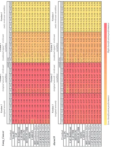
In the second set of experiments we compare empirically in the above two networks (four vari-ants for each as previously) and 6 sample sizes the following algorithms: semi-interleaved HITON-PC, MMHITON-PC, a version of HITON-PC where we pre-filter features by Benjamini FDR control (at FDR rate threshold of 5%) (Benjamini and Yekutieli, 2001), the true PC(T)set extracted from the data generating network (denoted as “True-PC” in Table 6), UAF (univariate association filtering) with Bonferroni correction, UAF with Benjamini FDR control, uncorrected UAF, “wrapped” UAF, RFE, and LARS-EN. Tables 6–9 provide support for the following conclusions:
(h) Due to strength of signal and redundancy of predictors, AUC reaches the theoretical maximum (provided by the generative network) very quickly and for all methods (Table 6).
L o w c la ss if ic a ti o n p e rf o rm a n c e H ig h c la ss if ic a ti o n p e rf o rm a n c e L u n g _ Ca n ce r F S m et h o d 1 0 0 2 0 0 5 0 0 1 0 0 0 2 0 0 0 5 0 0 0 1 0 0 2 0 0 5 0 0 1 0 0 0 2 0 0 0 5 0 0 0 1 0 0 2 0 0 5 0 0 1 0 0 0 2 0 0 0 5 0 0 0 1 0 0 2 0 0 5 0 0 1 0 0 0 2 0 0 0 5 0 0 0 T r u e -P C 1 .0 0 1 .0 0 1 .0 0 1 .0 0 1 .0 0 1 .0 0 1 .0 0 1 .0 0 1 .0 0 1 .0 0 1 .0 0 1 .0 0 0 .7 1 0 .7 2 0 .7 3 0 .7 2 0 .7 3 0 .7 5 0 .5 0 0 .5 0 0 .5 0 0 .5 0 0 .5 0 0 .5 0 U A F 1 .0 0 1 .0 0 1 .0 0 1 .0 0 1 .0 0 1 .0 0 0 .9 7 0 .9 9 1 .0 0 1 .0 0 1 .0 0 1 .0 0 0 .6 3 0 .6 7 0 .6 7 0 .6 8 0 .6 9 0 .7 2 0 .5 0 0 .5 1 0 .5 0 0 .5 0 0 .4 9 0 .5 1 U A F + B o n fe r r o n i 0 .9 7 1 .0 0 1 .0 0 1 .0 0 1 .0 0 1 .0 0 0 .9 4 1 .0 0 1 .0 0 1 .0 0 1 .0 0 1 .0 0 0 .6 0 0 .7 0 0 .7 4 0 .7 3 0 .7 4 0 .7 4 0 .5 0 0 .5 0 0 .5 0 0 .5 0 0 .5 0 0 .5 0 U A F + F D R 0 .9 8 1 .0 0 1 .0 0 1 .0 0 1 .0 0 1 .0 0 0 .9 5 1 .0 0 1 .0 0 1 .0 0 1 .0 0 1 .0 0 0 .6 1 0 .7 2 0 .7 4 0 .7 4 0 .7 4 0 .7 4 0 .5 0 0 .5 0 0 .5 0 0 .5 0 0 .5 0 0 .5 0 H I T O N -P C 0 .9 9 0 .9 9 1 .0 0 1 .0 0 1 .0 0 1 .0 0 0 .9 8 0 .9 9 1 .0 0 1 .0 0 1 .0 0 1 .0 0 0 .6 2 0 .6 7 0 .7 3 0 .7 3 0 .7 4 0 .7 4 0 .5 0 0 .4 9 0 .5 1 0 .5 1 0 .4 9 0 .4 9 H I T O N -P C -F D R 0 .9 7 0 .9 9 1 .0 0 1 .0 0 1 .0 0 1 .0 0 0 .9 4 0 .9 9 1 .0 0 1 .0 0 1 .0 0 1 .0 0 0 .6 1 0 .6 8 0 .7 3 0 .7 3 0 .7 4 0 .7 4 0 .4 9 0 .4 9 0 .4 9 0 .4 9 0 .4 9 0 .4 9 M M P C 0 .9 9 0 .9 9 1 .0 0 1 .0 0 1 .0 0 1 .0 0 0 .9 5 0 .9 9 1 .0 0 1 .0 0 1 .0 0 1 .0 0 0 .6 2 0 .6 7 0 .7 3 0 .7 3 0 .7 4 0 .7 4 0 .5 0 0 .4 9 0 .5 0 0 .5 0 0 .5 0 0 .5 0 L A R S -E N 0 .9 1 1 .0 0 1 .0 0 1 .0 0 1 .0 0 1 .0 0 0 .9 7 0 .9 8 1 .0 0 1 .0 0 1 .0 0 1 .0 0 0 .6 4 0 .7 0 0 .7 2 0 .7 1 0 .7 3 0 .7 4 0 .4 9 0 .5 0 0 .5 0 0 .5 0 0 .5 0 0 .5 1 R F E (r ed u ct io n 5 0 %) 0 .9 7 1 .0 0 1 .0 0 1 .0 0 1 .0 0 1 .0 0 0 .9 7 0 .9 9 1 .0 0 1 .0 0 1 .0 0 1 .0 0 0 .6 1 0 .6 5 0 .7 1 0 .7 0 0 .7 3 0 .7 4 0 .5 0 0 .5 0 0 .5 0 0 .5 0 0 .4 9 0 .5 0 R F E (r ed u ct io n 2 0 %) 0 .9 5 0 .9 9 1 .0 0 1 .0 0 1 .0 0 1 .0 0 0 .9 6 0 .9 8 1 .0 0 1 .0 0 1 .0 0 1 .0 0 0 .6 0 0 .6 8 0 .7 1 0 .7 1 0 .7 4 0 .7 4 0 .5 0 0 .5 0 0 .5 0 0 .4 9 0 .5 0 0 .5 0 U A F -K W-S V M (5 0 %) 0 .9 8 0 .9 9 1 .0 0 1 .0 0 1 .0 0 1 .0 0 0 .9 7 0 .9 9 1 .0 0 1 .0 0 1 .0 0 1 .0 0 0 .6 5 0 .6 9 0 .7 3 0 .7 1 0 .7 4 0 .7 4 0 .5 0 0 .5 0 0 .5 0 0 .5 0 0 .4 9 0 .5 0 U A F -K W-S V M (2 0 %) 0 .9 5 0 .9 9 1 .0 0 1 .0 0 1 .0 0 1 .0 0 0 .9 6 0 .9 8 1 .0 0 1 .0 0 1 .0 0 1 .0 0 0 .6 6 0 .7 1 0 .7 3 0 .7 2 0 .7 4 0 .7 4 0 .5 0 0 .5 0 0 .5 0 0 .4 9 0 .4 9 0 .5 1 U A F -S 2 N -S V M (5 0 %) 0 .9 4 0 .9 9 1 .0 0 1 .0 0 1 .0 0 1 .0 0 0 .9 4 0 .9 9 1 .0 0 1 .0 0 1 .0 0 1 .0 0 0 .5 8 0 .6 4 0 .7 4 0 .7 3 0 .7 4 0 .7 4 0 .5 0 0 .5 0 0 .5 0 0 .5 0 0 .5 0 0 .5 0 U A F -S 2 N -S V M (2 0 %) 0 .9 3 0 .9 8 1 .0 0 1 .0 0 1 .0 0 1 .0 0 0 .9 3 0 .9 8 1 .0 0 1 .0 0 1 .0 0 1 .0 0 0 .5 8 0 .6 7 0 .7 4 0 .7 3 0 .7 4 0 .7 4 0 .5 0 0 .5 0 0 .5 0 0 .4 9 0 .5 0 0 .5 0 A lar m
10 FS m
Lung_Cancer
FS method 100 200 500 1000 2000 5000 100 200 500 1000 2000 5000 100 200 500 1000 2000 5000
UAF 3.3 1.2 0.8 0.3 0.3 0.0 3.3 1.2 0.8 0.3 0.3 0.0 9.4 4.4 1.0 0.8 0.7 0.3
UAF+Bonferroni 13.9 6.1 1.5 1.0 0.9 0.2 17.6 8.4 1.8 1.0 1.0 0.5 24.9 19.9 6.7 2.4 1.0 1.0
UAF+FDR 9.2 2.5 0.9 0.5 0.4 0.0 13.4 4.8 1.3 0.9 0.8 0.0 24.0 16.2 3.5 1.3 1.0 0.8 HITON-PC 18.2 17.7 5.7 1.5 1.0 1.0 18.4 17.7 5.7 1.5 1.0 1.0 23.4 23.2 17.5 6.6 1.8 1.0 HITON-PC-FDR 19.3 18.5 5.7 1.5 1.0 1.0 19.2 18.5 5.7 1.5 1.0 1.0 24.7 23.3 17.9 6.6 1.8 1.0 MMPC 18.5 17.7 5.7 1.5 1.0 1.0 18.9 17.7 5.7 1.5 1.0 1.0 23.4 22.8 17.6 6.6 1.8 1.0 LARS-EN 19.9 14.2 8.8 7.9 3.6 1.0 15.9 18.6 10.0 10.0 3.7 1.6 22.8 21.5 18.3 13.4 9.4 10.7 RFE (reduction 50%) 20.7 15.9 9.4 6.1 4.1 1.0 18.8 14.6 13.3 9.2 3.2 1.6 21.1 15.9 7.6 8.6 14.8 12.8 RFE (reduction 20%) 21.9 17.1 10.5 12.5 4.9 2.6 18.7 18.8 11.0 9.1 3.7 2.3 15.6 18.1 8.3 14.3 16.9 12.3
UAF-KW-SVM (50%) 17.5 16.6 5.9 5.3 1.6 0.7 17.8 15.8 8.6 9.8 5.6 1.5 20.1 14.1 10.9 9.3 8.2 7.3
UAF-KW-SVM (20%) 21.0 18.8 10.5 8.3 2.6 0.7 19.1 18.7 10.7 13.2 6.4 1.2 20.5 14.3 12.4 8.1 6.9 7.2
UAF-S2N-SVM (50%) 20.8 17.1 6.0 7.6 2.5 1.3 17.6 16.7 8.4 7.1 7.0 1.9 16.6 15.4 15.6 11.5 8.3 4.9 UAF-S2N-SVM (20%) 23.1 19.9 9.4 10.5 5.1 1.8 20.5 18.5 10.4 11.3 7.0 0.7 19.4 14.8 15.4 12.3 6.6 5.5
Alarm10
FS method 100 200 500 1000 2000 5000 100 200 500 1000 2000 5000 100 200 500 1000 2000 5000
UAF 1.7 1.4 0.4 0.1 0.0 0.0 1.7 1.4 0.4 0.1 0.0 0.0 2.2 1.8 0.6 0.8 0.1 0.0
UAF+Bonferroni 4.1 2.7 1.4 1.0 0.5 0.0 4.7 3.2 1.5 1.1 0.7 0.2 5.0 4.4 2.7 1.4 1.0 0.5
UAF+FDR 3.3 2.2 0.8 1.0 0.3 0.0 4.3 2.8 1.4 1.1 0.5 0.0 4.9 3.8 2.4 1.2 0.9 0.2
HITON-PC 4.1 4.0 2.7 2.1 1.5 1.1 4.2 4.0 2.9 2.2 1.5 1.1 5.0 4.7 4.4 3.9 3.6 1.7
HITON-PC-FDR 4.6 4.2 3.2 2.3 1.7 1.0 4.8 4.3 3.2 2.3 1.7 1.0 5.5 4.7 4.4 4.2 3.6 2.1
MMPC 4.1 4.0 3.0 2.4 1.6 1.0 4.3 4.1 3.5 2.4 1.6 1.0 5.0 4.7 4.5 4.2 3.7 2.1
LARS-EN 3.8 3.8 1.7 1.7 1.5 1.4 4.4 4.1 2.5 2.2 1.9 1.4 4.6 4.6 4.6 3.5 2.2 2.0
RFE (reduction 50%) 4.1 3.7 2.1 1.9 2.3 1.5 4.8 4.7 3.2 3.3 2.6 1.8 4.6 4.9 5.2 4.6 4.2 3.6 RFE (reduction 20%) 4.1 3.7 2.4 2.7 2.1 1.8 5.0 4.4 3.4 3.2 2.3 2.0 5.0 5.3 5.0 4.5 3.7 3.3 UAF-KW-SVM (50%) 3.8 3.8 2.2 0.8 0.9 0.4 4.8 3.6 2.4 2.2 1.4 0.1 3.8 4.2 3.4 2.1 2.2 0.8
UAF-KW-SVM (20%) 4.0 3.2 2.4 1.1 0.4 0.0 4.2 3.6 2.4 1.9 1.2 0.0 4.2 4.3 2.7 2.8 1.9 1.2 UAF-S2N-SVM (50%) 3.5 3.6 2.1 1.0 0.8 0.4 4.7 3.8 2.2 2.1 1.5 0.2 5.1 4.4 4.3 3.5 2.7 1.0 UAF-S2N-SVM (20%) 4.3 3.5 2.6 1.3 0.5 0.0 4.9 3.7 2.5 1.9 1.7 0.2 5.0 4.5 3.6 3.0 2.5 1.4
Version 1 (original network)
Version 2 (original network + irrelevant
variables)
Version 3 (weakened signal + irrelevant
variables)
sample size
Version 1 (original network)
Version 2 (original network + irrelevant
variables)
Version 3 (weakened signal + irrelevant
variables)
sample size
Small number of false negatives Large number of false negatives
Table 7: Number of false negatives in the parents and children set for selected features. HITON-PC, HITON-PC- FDR, and MMPC are applied with max-k=2. For Version 4 of the network the parents and children set is empty since there are no relevant variables. The color of each table cell denotes number of false negatives with yellow (light) corresponding to smaller values and red (dark) to larger ones.
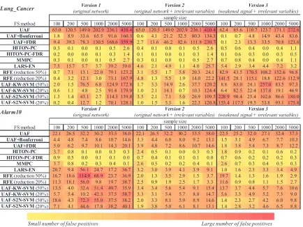
separation (i.e., 1-2 false negatives and zero false positives) at sample size 1,000 and higher (Table 8). No other method simultaneously minimizes false positives and false negatives as GLL.
(j) In the setting of strong signal with irrelevant features, simple UAF has the least false negatives in very small samples (Table 7) and the largest number of false positives (Table 8).
Lung_Cancer
FS method 100 200 500 1000 2000 5000 100 200 500 1000 2000 5000 100 200 500 1000 2000 5000
UAF 65.0 120.5 149.0 202.9 236.1 410.4 65.0 120.5 149.0 202.9 236.1 410.4 62.4 85.6 110.7 123.7 171.1 272.6
UAF+Bonferroni 1.8 8.9 33.6 65.5 91.6 160.3 0.6 4.1 21.2 52.5 80.3 134.3 0.1 0.7 4.8 14.9 43.4 83.6
UAF+FDR 9.4 39.3 78.3 130.5 168.6 359.9 2.7 13.6 46.2 82.6 111.8 230.7 0.1 2.3 13.3 33.5 70.8 123.6
HITON-PC 0.3 0.1 0.0 0.1 0.5 2.6 0.4 0.1 0.0 0.1 0.5 2.6 0.5 0.6 0.4 0.0 0.4 1.1
HITON-PC-FDR 0.2 0.0 0.0 0.1 0.3 1.4 0.1 0.1 0.0 0.1 0.3 1.4 0.1 0.6 0.3 0.0 0.3 0.5
MMPC 0.3 0.1 0.0 0.1 0.5 2.7 0.3 0.1 0.0 0.1 0.5 2.7 0.7 0.8 0.4 0.0 0.4 1.1
LARS-EN 7.5 15.7 5.7 3.7 39.2 59.0 4.6 2.1 4.9 1.1 4.0 25.7 5.4 2.9 3.4 4.4 7.2 3.2
RFE (reduction 50%) 0.7 7.1 13.1 22.0 79.1 123.2 3.1 5.5 1.7 5.8 20.3 24.1 82.9 43.5 170.5 108.2 152.6 96.8 RFE (reduction 20%) 0.4 3.2 12.1 3.0 73.1 167.9 4.8 1.3 5.5 1.9 14.0 22.2 141.5 28.1 115.1 18.8 122.6 112.9 UAF-KW-SVM (50%) 2.0 1.5 76.5 6.8 124.9 172.8 1.7 3.3 14.9 2.6 37.7 120.2 8.8 83.0 24.1 257.0 83.5 97.3 UAF-KW-SVM (20%) 0.6 1.1 4.8 2.5 91.4 179.9 1.0 2.1 14.1 0.7 10.3 124.4 6.4 82.5 22.4 137.8 19.1 46.9 UAF-S2N-SVM (50%) 1.3 1.4 43.1 2.7 114.3 139.8 3.5 2.1 7.1 5.0 26.9 109.5 228.9 98.4 25.4 102.6 86.6 180.0 UAF-S2N-SVM (20%) 0.2 0.4 12.7 1.2 70.1 128.1 1.0 1.5 5.3 1.6 22.3 120.8 153.4 117.5 19.5 53.8 93.1 175.8
Alarm10
FS method 100 200 500 1000 2000 5000 100 200 500 1000 2000 5000 100 200 500 1000 2000 5000
UAF 22.1 26.5 32.2 30.2 33.5 38.0 22.1 26.5 32.2 30.2 33.5 38.0 22.5 25.2 32.0 27.1 32.4 37.3 UAF+Bonferroni 4.4 4.8 7.4 8.6 10.7 14.6 3.3 4.4 6.0 8.0 9.2 13.1 1.5 3.1 4.9 6.7 7.7 10.3
UAF+FDR 5.0 6.2 9.7 10.1 14.3 20.1 3.9 4.8 7.2 8.6 10.7 14.6 1.8 3.8 5.4 7.3 8.7 12.2
HITON-PC 3.7 0.8 0.1 0.0 0.3 0.3 2.4 0.5 0.1 0.0 0.3 0.3 1.8 0.9 0.2 0.1 0.6 0.2
HITON-PC-FDR 0.9 0.5 0.0 0.1 0.1 0.0 0.7 0.4 0.1 0.1 0.1 0.0 0.7 0.6 0.2 0.2 0.2 0.3
MMPC 3.7 0.8 0.2 0.3 0.4 0.1 2.6 0.5 0.2 0.2 0.4 0.1 2.6 0.7 0.3 0.4 0.5 0.3
LARS-EN 20.7 9.4 56.1 24.7 17.2 36.7 3.2 3.0 3.9 4.1 3.9 9.1 1.0 1.6 2.3 3.3 3.4 4.9
RFE (reduction 50%) 16.7 18.6 114.9 68.9 23.7 36.9 2.0 1.3 3.5 2.9 1.5 3.7 19.7 1.4 1.3 1.6 1.9 2.9 RFE (reduction 20%) 11.3 18.1 56.0 9.8 19.7 38.7 2.5 0.9 1.9 2.5 1.7 3.3 11.6 0.9 0.8 1.1 1.5 2.7 UAF-KW-SVM (50%) 13.5 4.0 32.6 51.4 49.7 35.9 3.4 3.4 5.6 5.4 9.1 15.4 13.7 3.7 4.4 5.7 7.6 10.6 UAF-KW-SVM (20%) 5.7 5.4 10.2 42.3 37.5 58.7 3.3 3.1 5.4 5.7 8.8 14.7 5.6 3.3 4.9 5.2 7.3 9.0
UAF-S2N-SVM (50%) 18.6 4.3 72.3 55.0 37.5 38.2 2.0 3.3 8.1 5.9 8.9 14.6 1.4 2.3 2.7 4.2 6.0 9.8 UAF-S2N-SVM (20%) 7.1 4.1 44.6 17.8 38.2 40.1 1.9 3.8 5.0 6.1 8.1 13.1 1.4 2.8 3.2 4.6 6.5 8.8
Version 1
(original network)
Version 2
(original network + irrelevant variables)
Version 3
(weakened signal + irrelevant variables) sample size
Version 1
(original network)
Version 2
(original network + irrelevant variables)
Version 3
(weakened signal + irrelevant variables) sample size
Small number of false positives Large number of false positives
Table 8: Number of false positives (within weakly relevant variables) in the parents and children set for selected features. HITON-PC, HITON-PC-FDR, and MMPC are applied with
max-k=2. For Version 4 of the network there are no weakly relevant variables. The color of each
table cell denotes number of false positives with yellow (light) corresponding to smaller values and red (dark) to larger ones.
MMPC performing similarly) achieves excellent false positive rates better than those by FDR not only for weakly relevant but also for irrelevant features.
(l) PC augmented with FDR pre-filtering behaves almost identically as regular HITON-PC except for the case with only irrelevant features in the data where HITON-HITON-PC without FDR admits a few false positives (Table 9).
(m) State-of-the-art feature selection methods are prone to select very large numbers of irrelevant features (Table 9).
higher regardless of sample size. Given enough sample size (∼1,000 or more in the data tested), and
by choosing 5% as the nominalαfor all conditioning independence tests executed, the algorithm fully eliminates irrelevant features from its output without incurring a penalty in false negatives, even when irrelevant features are the majority among observed features. Parameter max-k controls the false positives due to both weakly relevant and irrelevant features. The false positive rate in this worst-case situation is in the presented experiments∼5/8,000 = 0.000625 which is much better
than what the conservative Bonferroni-adjustedαguarantees, and without incurring false negatives (as both Bonferroni and FDR methods do). Both established feature selectors such as variants of UAF and newer ones are very sensitive to irrelevant features and produce large numbers of false positives. Given the attractive characteristics of FDR-augmented HITON-PC, we evaluate it with real data sets in Section 5.
4. Theoretical Analysis of GLL
In the present section we provide a theoretical analysis of the Generalized Local Learning algo-rithms.
4.1 Determinants of Quality of Statistical Decisions and Computational Tractability. Parameters max-k and h-ps
On a rather superficial level when conditioning sets are large enough, statistical tests become less reliable. For example, as explained in Aliferis et al. (2010), cells in contingency tables used to calculate p-values of discrete tests of independence (such as the widely-used G2or X2test) become scarcely populated and this leads to unreliable test results. This motivates the heuristic practice of considering as unreliable and not executing a test in which the sample size is less than: (“number of cells to be fitted”·h-ps), with parameter h-ps set to 10 by default in the PC algorithm (Spirtes
et al., 2000) and 5 in GLL instantiations. Recall from Aliferis et al. (2010) that h-ps stands for “heuristic power size” and denotes the smallest sample size per cell in the contingency table of a reliable conditional test of independence. Moreover, when the conditioning set size is large enough to block all paths between a weekly relevant variable and the target, there is no need to exceed this conditioning set size because the resulting tests are redundant and the operation of the algorithm becomes unnecessarily slow. Thus it seems reasonable that we would wish to restrict the condition-ing set size to not exceed this sufficient blockcondition-ing size. This is accomplished by settcondition-ing the value of parameter max-k. We will see however that max-k has a much more elaborate function than simply “trimming away” excessive computations.
In reality things are significantly more complicated because, as first pointed out by Spirtes et al. (2000), statistical reliability of a single test is a misleading concept in the context of com-plex constraint-based algorithms such as GLL. Standard statistical considerations of the type of testing a hypothesis once do not carry over well to the constraint-based algorithm setting. Similarly, running time is also a complex function of direct or indirect restrictions placed on number of tests and the number of variables with which to build such tests (i.e., the size of TPC(T)).
execute the test and assume independence by default, we will surely miss it. In the context of many
tests however, the notion of single-test reliability for S no longer applies. For example, when we
consider a test that has the potential to reject S from TPC(T)(where it was placed previously by a
different test), by allowing the conditioning test size to grow large, the power is reduced (assuming
monotonic association of S through the potentially multiple paths connecting S with T ). Hence, we need to preserve the combined power (i.e., combination of individual powers of all tests applied to
S) in order to not eliminate S from TPC(T). Although these tests are highly correlated and com-bined power is larger than the product of powers of the same set of tests performed on independent samples, still the more tests are executed the smaller the combined power and the larger the pos-sibility of falsely eliminating S becomes. The parameter h-ps partially controls power because the larger it is, the smaller number of tests (that would eliminate S) are executed. However h-ps should not be too large either because a strongly relevant S will not be included in TPC(T)in the first place. Parameter max-k also controls in part the number of tests allowed. Max-k does not fully determine the number of tests because it specifies the dimensionality of allowed tests, not their total number. As max-k grows, more tests for eliminating S from TPC(T)are executed, thus the combined power drops. In summary, for a given distribution the number of tests performed is affected by h-ps, max-k and the size of TPC(T).
So far the discussion has centered on one type of conditional independence test, that is, tests where the candidate member of PC(T), X , is a strongly relevant feature (type 1). This is the first of four types of conditional tests. The other three are: conditional independence tests where the candidate member of PC(T), X , is a weakly relevant feature and some paths with T are not blocked by the conditioning set (type 2a), conditional independence tests where the candidate member of
PC(T), X , is a weakly relevant feature and all paths with T are blocked by the conditioning set (type 2b), and finally conditional independence tests where the candidate member of PC(T), X , is an irrelevant feature (type 3).
The quality of conditional tests of the first type is determined by the power of the association of
X with T given the conditioning set. Since not one but potentially many such tests are conducted,
the combined power of all such tests determines whether X will be selected and stay in the TPC(T)
set. For example, variable X (a true member of PC(T)) will be considered for inclusion in TPC(T)
by HITON-PC with probability = power of detecting¬I(X,T)given the available sample size and test employed. However for X to stay in TPC(T) until the algorithm terminates, and assuming
B, C have entered TPC(T), none of the tests I(X,T|B), I(X,T|C), I(X,T|{B,C})must conclude independence. The power or each one of these tests can be lower or higher than the power of I(X,T)and the combined power can quickly diminish, however several mitigating factors prevent this from happening. First, when using linear tests under common distributional assumptions such as multivariate normality, the necessary sample size to achieve desired level of power grows linearly to number of variables in the conditional set. Second, as explained earlier, conditional independence tests of the same variable and T in the same sample are highly correlated. Third, controlling the number of members of TPC(T) by a good heuristic inclusion function reduces the total number of tests; such control occurs indirectly by putting first the true members of PC(T) or members that block many variables. Fourth, the order of executing the tests and constructing conditioning sets is important for reducing the number of tests performed on strongly relevant variables. This is exemplified in semi-interleaved HITON-PC where new entrants in TPC(T)are tested before current
Returning our attention to the quality of statistical decisions for weakly relevant variables, we observe that when a conditioning set does not block all paths to/from T either for inclusion or for elimination purposes (type 2a), we are sampling under the alternative hypothesis (i.e., there exists association) and the determining factor for failing to reject the weakly relevant feature is the combined power which is determined by the same factors as elaborated for strongly relevant variables previously. The combined probability for rejection may be small for similar reasons as type 1 conditional independence tests (albeit higher than for strongly relevant features due to the fact that under a good inclusion heuristic weakly relevant features enter TPC(T)later than strongly relevant ones and thus more tests are applied on each weakly relevant than on each strongly relevant feature on average).
However, when the conditioning set blocks all paths from/to T (type 2b), then we sample under
the null hypothesis and the determining factor shifts from the combined power to the combined α (i.e., statistical significance). Given that the α for each conditional test is typically low (i.e., 5% or smaller) and that as the number of tests under the null increases, the combinedαdrops up to exponentially fast, and eliminating weakly relevant features occurs with high probability as the number of applied tests increases. In HITON-PC, the smaller is h-ps, the easier it is to include a weakly relevant feature (based on univariate association heuristic), whereas max-k does not affect this function. In terms of rejecting a weakly relevant feature in TPC(T), the larger max-k and the smaller h-ps become, the easier it is to eliminate a weakly relevant feature.
The quality of statistical decisions for type 3 of conditional independence tests, that is for irrel-evant variables, is determined by the combinedαsince we always test under the null hypothesis. Because the combinedαdrops fast as the number of tests applied to each irrelevant variable (and these tests are abundant when even a handful of variables have been admitted in TPC(T)), the com-bined probability for admitting and not rejecting irrelevant variables is exceedingly small. However when no strongly (and thus no weakly) relevant feature exists, conditioning sets inside the TPC(T)
set become smaller as irrelevant variables are eliminated from it with the end result of leaving a small number of “residual” irrelevant features in the final output as evidenced in the simulation experiments of Section 3. By pre-filtering variables with an FDR filter (Benjamini and Yekutieli, 2001; Benjamini and Hochberg, 1995), we not only gain the security that if the data consists exclu-sively of irrelevant variables fewer or no false positives will be returned, but also we can use max-k to control sensitivity and specificity trading weakly relevant false positives for strongly relevant true positives and vice versa (i.e., without worrying about adversely trading off irrelevant features).
Finally, the total number of tests is determined by both parameters h-ps and max-k, in a non-monotonic manner. That is, whenever h-ps is extremely large it effectively disallows most tests and the algorithm quickly terminates returning the empty set regardless of max-k. For medium/small values of h-ps, more tests are executed, more variables enter TPC(T), and many tests are executed before TPC(T)is finalized. Max-k modifies this number by potentially restricting the number of tests. When h-ps is very small, tests are allowed with very large conditioning tests and as long as
Lung_Cancer max-k HITON-PC MMPC max-k HITON-PC MMPC max-k # of fn # of fp
1 4,028 5,683 1 7,257 8,900 1 1 13
Target variable #1 2 12,328 14,577 2 33,018 38,892 2 1 0
3 73,554 77,885 3 277,922 294,211 3 1 0
4 250,560 259,099 4 1,181,889 1,225,682 4 3 0
Alarm10 max-k HITON-PC MMPC max-k HITON-PC MMPC max-k # of fn # of fp
1 457 490 1 545 585 1 1 2
Target variable #199 2 470 496 2 608 652 2 1 0
3 491 521 3 692 752 3 1 0
4 496 527 4 717 782 4 1 0
* Results are same for HITON-PC and MMPC for number of false positives and false negatives Number of members in
PC set = 6
Number of conditional independence tests
Cost of conditional independence tests
Number of false positives (fp) and false negatives (fn)*
Number of members in PC set = 26
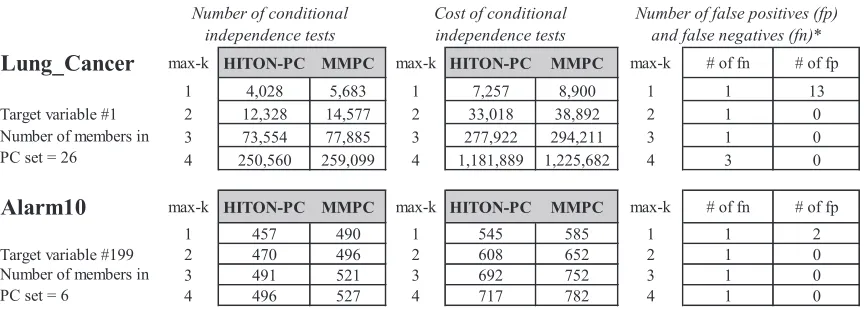
Figure 2: Efficiency of HITON-PC versus MMPC.
4.2 Efficiency and Heuristic Robustness of HITON-PC Versus MMPC
Figure 2 presents the number and cost2 (proportional to time) of conditional independence tests performed by semi-interleaved HITON-PC versus MMPC in the 2,000-sample data set from the
Alarm10 and Lung Cancer networks. As can be seen, HITON-PC performs fewer tests on average
while achieving the same performance as MMPC. We notice that the max-min association heuristic closely reflects the logic behind the combined probability for error for the weakly relevant features. MMPC when testing under the alternative hypothesis (i.e., strongly relevant features, or unblocked weakly relevant ones) requires measuring all relevant associations, whereas HITON requires just the univariate ones for inclusion purposes. However semi-interleaved HITON tries to eliminate the newly included variable immediately upon inclusion and thus effectively conducts a similar number of tests as MMPC. Both algorithms when testing under the null hypothesis (irrelevant or fully-blocked weakly relevant features) on average execute the same number of tests. The max-min association inclusion heuristic is a priori more prone to basing its decisions for inclusion in
TPC(T)on less statistically reliable criteria. This is because the more associations are considered and the larger the conditioning sets are, the higher variance in the minimum association estimates is expected, making the maximum of such associations over all variables considered more prone to sampling error (i.e., it is likely to be overfitted to the sample). Because of better robustness of the univariate association relative to the weakest association over many conditional associations true members of PC(T)may enter the TPC(T)set earlier. However both HITON-PC and MMPC exhibit similar performance in real and simulated data sets, demonstrating that the theoretical problem with max-min association is in practice very rare.
4.3 Synthesis and Problems for Inclusion Heuristics; Constructing New Inclusion Heuristics
A problem when inducing local neighborhoods and particularly Markov blankets is that of
informa-tion synthesis. The problem consists of a variable X that is not in PC(T)having higher association (univariate or conditional on some subsets) with T than members of PC(T)(for a concrete example see Figure 13). We will call such variables, synthesis variables. Synthesis variables were identified
as major problems for algorithms such as IAMB (Tsamardinos and Aliferis, 2003; Tsamardinos et al., 2003a) or GS (Margaritis and Thrun, 1999) that induce Markov blankets and do so by condi-tioning in their inclusion phase on all variables in the tentative MB(T). Because of the requirement to condition on all variables in the tentative MB(T), the sample requirements grow exponentially fast to the size of the tentative MB(T)and thus it is absolutely imperative to keep out of it synthesis variables since they unnecessarily increase the sample requirements to the point that the algorithm may need to stop executing conditional independence tests (and either halt or output the tentative
MB(T)as best but flawed estimate of the true MB(T)).
With regards to GLL algorithms, most efficient operation is achieved when the variables that alone or in combination have the property that block the largest fraction of weakly relevant variables, enter first in TPC(T)(even if they are not strongly relevant themselves). Synthesis variables may or may not have this property, so synthesis may or may not be a problem for a specific GLL algorithm based on characteristics of the specific data in hand.
Construction of new inclusion heuristics may be required in difficult cases where the univari-ate and max-min heuristics do not work well leading to very slow processing time and very large
TPC(T)sets, in order to make operation of local learning tractable. In practice, both the univariate and max-min association heuristics work very well with real and simulated data sets, so we do not pursue here implementation and testing new heuristics in artificial problems, although we recog-nize the possibility of such need in future problematic data distributions. We outline here, in broad strokes, general strategies for creating new inclusion heuristics for such cases:
1. Random heuristic search informed by standard heuristic values. This strategy is based on using one of the usual heuristics to rank candidate variables and making selection decisions based on random selection of a candidate variable with probability proportional to the original heuristic value. This enables using the older heuristic as a starting point but allowing occa-sionally deviations from it to explore the possibility that lower-ranked candidates may have better potential as blocking variables. A simulated-annealing determination of probability of selection (or other efficient stochastic search algorithms) can be pursued as well.
2. Constructing new heuristic functions by observing blocking capability (in terms of candidate variables blocked by conditioning sets in which V is a member) or probability of a
vari-able V to remain in TPC(T). The empirical observations can be collected from a variety of
tractable sources: either from a single incomplete run of the algorithm (i.e., without waiting to terminate), or in other data sets characteristic of the domain, or in multiple runs on smaller (randomly chosen) subsets of the original feature set. The new heuristic function F can be constructed as the conditional probability:
F(Vi) =P(Vi∈TPC(T)|h(Vi))
where h(Vi) is the original heuristic value of variable Vi, or the proportion of candidates
blocked by a conditioning set containing Vi:
F(Vi) = M
∑
k=1Nk(Vi)/M
where Nk(Vi)is the number of candidate variables blocked by a conditioning set that contains
3. Exploiting known domain structure. When properties of the causal structure of the data gen-erating structure and/or distributional characteristics are known, one can use this information alone or in conjunction with the previous two strategies to derive more efficient heuristics.
We note that developing an inclusion heuristic that leads to efficient execution of GLL is not always feasible since the very problem of finding the features with direct edges with the target is intractable in the worst case (e.g., consider a graph that is fully connected). In some cases, as we will show in Section 6, it is possible to transform an intractable local learning problem into a tractable
one by employing a global learning strategy (i.e., exploiting asymmetries in connectivity).
4.4 Inductive Bias of GLL
Informally the inductive bias of GLL is that it seeks a balance of false negatives for strongly relevant variables with false positives for weakly relevant and irrelevant variables. The main regulating parameters (for standard inclusion heuristics, elimination and interleaving strategies) are h-ps and
max-k. In practice, the algorithms tested in our work to date reveal higher sensitivity to max-k and
thus at first approximation we treat optimization of this parameter as having higher priority. Smaller
max-k empirically decreases false negatives and increases false positives overall. Larger max-k
increases the false negatives and decreases the false positives. GLL in moderate to large samples achieves small numbers of false negatives and small numbers of false positives. In very small samples GLL prefers false positive errors than false negative ones when max-k is small. This occurs because given some evidence in favor of PC(T)membership (provided by lower-dimensional and thus more sample efficient) tests of a variable X but no reliable proof to the contrary (provided by omitted higher-dimensional and thus unreliable tests), the algorithm outputs X as member of PC(T). A similar behavior exists for the MB(T)versions (with respect to MB(T)membership). Notice that as max-k grows many more tests can be executed provided that a liberal h-ps is chosen, and these tests can be used to eliminate both weakly relevant as well as strongly relevant features in TPC(T). The choice of a more liberal h-ps default value in GLL (compared to the more stringent value in the published implementation of PC algorithm) allows a more effective control of the tradeoff between false positives and false negatives in small samples by changing values of max-k.
By contrast, the SGS and PC algorithms (Spirtes et al., 2000) given no evidence in favor of membership of X in PC(T) and no reliable proof to the contrary, assumes that X has a common edge with T . IAMB (Tsamardinos and Aliferis, 2003; Tsamardinos et al., 2003a) to the contrary, given some reliable evidence in favor of a variable X belonging to MB(T)but no reliable proof to the contrary, outputs X as member of MB(T)if X is in the tentative Markov blanket TMB(T)and is agnostic with respect to membership in MB(T)if X is outside TMB(T). Bayesian scoring methods in small samples are dominated by their priors and typically they prefer sparse networks which lead to fewer false positives and more false negatives.
4.5 Reasons for Good Performance of Non-Symmetry Corrected Algorithms
A
T
C B
D
A
T C B
E
D A
T C
B T
B
(H)
T
A B (H)
T
A B
Real Apparent
1 2 3
4 5
Figure 3: Scenarios explaining good empirical performance of PC(T)set for classification.
4.6 Reasons for Good Performance of the PC(T)Set Instead of the MB(T)Set for Classification
According to the theoretical results summarized in Aliferis et al. (2010), under broad assumptions spouses are needed for optimal classification performance. Given that in the majority of data sets tested in Aliferis et al. (2010) as well as the experiments in Section 2 of the present paper, when the set of parents and children is used instead of MB(T)it produces equal or almost equal performance, more compact feature sets and faster feature selection times than inducting the full MB(T)(i.e., both
PC(T) and MB(T) estimated under the same assumptions of the theory that predicts that MB(T)
is needed for optimal feature selection). In this sub-section we provide likely explanations for the empirically excellent performance of substituting the set PC(T)in place of MB(T)for classification (apart from the obvious possibility that spouses may be much fewer and with smaller predictive value than parents and children). Figure 3 describes visually five plausible scenarios explaining the phenomenon.