Vol. 10, No. 2, 2018 Article ID IJIM-00730, 14 pages Research Article
Numerical Simulation of 1D Linear Telegraph Equation With
Variable Coefficients Using Meshless Local Radial Point Interpolation
(MLRPI)
E. Shivanian ∗†, S. Abbasbandy ‡, A. Khodayari§
Received Date: 2015-07-26 Revised Date: 2016-10-11 Accepted Date: 2017-10-16 ————————————————————————————————–
Abstract
In the current work, we implement the meshless local radial point interpolation (MLRPI) method to find numerical solution of one-dimensional linear telegraph equations with variable coefficients. The MLRPI method, as a meshless technique, does not require any background integration cells and all integrations are carried out locally over small quadrature domains of regular shapes, such as lines in one dimensions, circles or squares in two dimensions and spheres or cubes in three dimensions. Weak form formulation of the discretized equations has been constructed on local subdomains, hence the domain and boundary integrals in the weak form methods can easily be evaluated over the regularly shaped sub-domains by some numerical quadratures. Radial basis functions augmented with monomials are used in to create shape functions. These shape functions have delta function property. Also the time derivatives is eliminated by using two-step finite differences approximation. Two illustrative numerical examples are given to show the stability and accuracy of the present method.
Keywords: Meshless local radial point interpolation (MLRPI); Radial basis function; Variable coeffi-cient; Telegraph equation.
—————————————————————————————————–
1
Introduction
T
hsolutions of the second order hyperbolic tele-is paper is dedicated to study the numerical graph equation. The telegraph equation is impor-tant for modeling several relevant problems such∗Corresponding author. [email protected],
Tel.:+98(912)6825371
†Department of Applied Mathematics, Imam Khomeini
International University, Qazvin, Iran.
‡Department of Applied Mathematics, Imam Khomeini
International University, Qazvin, Iran.
§Department of Applied Mathematics, Imam Khomeini
International University, Qazvin, Iran.
as signal analysis [25], wave propagation [48], vi-brational systems [10], random walk theory [6], mechanical systems [45] and etc. Recently, in-creasing attention has been paid to the devel-opment, analysis, and implementation of stable methods for the numerical solutions of second-order hyperbolic equations. There have been many numerical methods for hyperbolic equa-tions, such as the finite difference, the finite ele-ment, and the collocation methods, etc. see [3,4, 12,11,13,14,16,17,18,24,31,32,33,34,35,46] and literatures are therein.
One of the most important advances in the field of numerical methods was the development
of the finite element method (FEM) in the late 1950s. For a long time, FEM has been a stan-dard tool for numerically solving different engi-neering problems. But The main shortcoming of FEM is that this numerical method rely on meshes or elements. Therefore, the meshless or meshfree method is proposed as one such nu-merical technique to overcome this shortcoming. Meshless methods have been developed in the past decade, and significant progress has been achieved recently for numerical computations of wide ranging engineering problems. These mesh-less methods do not require mesh for discretisa-tion of problem domains, and they construct the approximate functions only via a set of nodes so-called field nodes where no element is required for approximation of functions [28]. In general, the meshless methods can be grouped into two cate-gories based on using or not using integration or based on computational modelling [27]. The first category involves methods that do not require in-tegration and are based on the strong forms of partial differential equations (PDEs) such as the meshless collocation method based on radial basis functions (RBFs) [26, 15,29, 20] and the mesh-less collocation method based on boundary par-ticle method (BPM) [21]. The second category includes meshless methods based on the weak forms of PDEs such as the element free Galerkin (EFG) method [8, 9]. In addition, a meshless method based on the combination of the strong form and weak form has also been developed and is known as the meshless weakstrong (MWS) form method. In the meshless strong form methods, usually the PDEs are discretized at nodes by the collocation technique and it is simple to imple-ment. However, the meshless strong form meth-ods have obvious shortcomings. For example, they are often numerically unstable and less ac-curate. The second category consists of meshless methods based on the weak forms of PDEs, in-cluding global weak form and local weak form. The meshless methods based on the weak form have very attractive merits. They exhibit very good stability and excellent accuracy. The rea-son is probably that the weak form can smear the computational error over the integral domain and control the error level [28]. The weak forms are used to derive a set of algebraic equations through
a numerical integration process using a set of quadrature domain that may be constructed glob-ally or locglob-ally in the domain of the problem. In the global weak form methods, global back-ground cells are needed for numerical integration in computing the algebraic equations. To avoid the use of global background cells, a so-called lo-cal weak form is used to develop the meshless local Petrov-Galerkin (MLPG) and meshless lo-cal radial point interpolation (MLRPI) methods [44,42,43,5,41,22,1,2,38,39,40]. When a local weak form is used for a field node, the numerical integrations are carried out over a local quadra-ture domain defined for the node, which can also be the local domain where the test (weight) func-tion is defined. The local domain usually has a regular and simple shape for an internal node (such as sphere, rectangular, etc.), and the inte-gration is done numerically within the local do-main. Hence the domain and boundary integrals in the weak form methods can easily be evaluated over the regularly shaped sub-domains(spheres in 3D or circles in 2D) and their boundaries.
According to the numerical results obtained by the MLRPI method, it seems this method can be employed as practical and effective numerical technique to solve telegraph equations with vari-able coefficients.
Let Ω = [0,1] and consider the 1D linear tele-graph equation:
∂2u(x, t)
∂t2 + 2α(x, t)
∂u(x, t) ∂t +
β2(x, t)u(x, t) =A(x, t)∂
2u(x, t)
∂x2 +g(x, t), (x, t)∈ Ω × [0, T], (1.1)
with the initial and boundary conditions:
u(x,0) = g1(x), ∂u
∂t(x,0) = g2(x), (1.2) u(0, t) = φ0(t), u(1, t) = φ1(t), t≥0 (1.3)
where g, g1, g2, φ0, φ1 are known functions, the function u is unknown and α, β, A are variable coefficients.
2
Numerical scheme
2.1 Finite differences approximation
In the proposed method, we employ a time-stepping scheme to approximate the time deriva-tive. For this purpose, the following finite differ-ence approximations of orderO(∆t)2 are used:
∂2u(x, t) ∂t2 ∼=
1 ∆t2
(
u(k+1)(x) −2u(k)(x) ,
+u(k−1)(x)
)
, (2.4)
∂u(x, t) ∂t ∼=
1 2 ∆t
(
u(k+1)(x) − u(k−1)(x)
) .
(2.5) By using Crank-Nicholson scheme, we have:
u(x, t) ∼= 1 3
(
u(k+1)(x) +u(k)(x)
+u(k−1)(x)), ∂2u(x, t)
∂x2 ∼= 1 3
(
∂2u(k+1)(x, t) ∂x2
+∂
2u(k)(x, t)
∂x2 +
∂2u(k−1)(x, t) ∂x2
) ,
(2.6)
whereuk(x) = u(x, k∆t).
Using the above approximations, Eq. (1.1) be-comes:
1 ∆t2
(
u(k+1)(x) −2u(k)(x) + u(k−1)(x))
+ α ∆t
(
u(k+1)(x) − u(k−1)(x))
+β 2
3
(
u(k+1)(x) +u(k)(x) +u(k−1)(x))
−A
3
(
∂2u(k+1)(x) ∂x2 +
∂2u(k)(x) ∂x2
+∂
2u(k−1)(x)
∂x2 )
= 1 3
(
g(k+1)(x) + g(k)(x) + g(k−1)(x)).
(2.7) In this paper for simplicity, telegraph equation is considered with variable coefficients α(x, t) =
x2, β(x, t) =x, A(x, t) = 1 +x, therefore
1 ∆t2
(
u(k+1)(x) −2u(k)(x) + u(k−1)(x))
+ x 2
∆t (
u(k+1)(x) − u(k−1)(x))
+x 2
3
(
u(k+1)(x) +u(k)(x) +u(k−1)(x))
−1 +x
3
(
∂2u(k+1)(x) ∂x2 +
∂2u(k)(x) ∂x2
+∂
2u(k−1)(x)
∂x2 )
= 1 3
(
g(k+1)(x) + g(k)(x) + g(k−1)(x)),
(2.8) thus
1 ∆t2 u
(k+1) + (
1 ∆t +
1 3
)
x2u(k+1)
−1
3
∂2u(k+1)(x) ∂x2 −
1 3 x
∂2u(k+1)(x) ∂x2 = 2
∆t2 u
(k) − 1 3x
2u(k)
+1 3
∂2u(k)(x) ∂x2 +
1 3 x
∂2u(k)(x) ∂x2
− 1
∆t2 u
(k−1) + (
1 ∆t −
1 3
)
x2u(k−1)
+1 3
∂2u(k−1)(x) ∂x2 +
1 3x
∂2u(k−1)(x) ∂x2 +1
3
(
g(k+1)(x) + g(k)(x) + g(k−1)(x)).
(2.9)
2.2 Approximation of field variables
using radial point interpolation method
functions.
Consider a continuous functionu(x) defined in a domain Ω, which is represented by a set of field nodes. The u(x) at a point of interest x is ap-proximated in the form of
u(x) = ∑ni= 1 Ri(x)ai
+∑mj= 1 pj(x)bj = RT(x)a + PT(x)b, (2.10) where Ri(x) is a radial basis function (RBF), n is the number of RBFs, pj(x) is monomial in the space coordinatexand mis the number of poly-nomial basis functions. The pj(x) in Eq. (2.10) is, in general, chosen in a top-down approach from the Pascal triangle, so that the basis is complete to a desired order and a complete basis is usually preferred. For 1D problems, We use
PT(x) = {1, x, x2, x3, ..., xm}, (2.11)
for 2D problems, We shall have
PT(x) = PT(x, y) =
{
1, x, y, xy, x2, y2, ..., xm, ym}, (2.12)
and etc.
When m = 0, only RBFs are used. Otherwise, the RBF is augmented with m polynomial ba-sis functions. Coefficientsai and bj are unknown which should be determined. There are a number of types of RBFs, and the characteristics of RBFs have been widely investigated [26,19,37]. In this paper we consider the thin plate spline (TPS) as radial basis functions in Eq. (2.10). This RBF is defined as follows:
R(x) = r2s ln(r), s = 1, 2, 3, .... (2.13)
Since R(x) in Eq. (2.13) belongs to C2s−1 (all continuous function to the order 2s−1), so order thin plate splines must be used for higher-order partial differential operators. For the second-order partial differential equation (1.1), s= 2 is used for thin plate splines (i.e., second-order thin plate splines). In the radial basis function Ri(x), the variable is only the distance between the point of interest x and a node at xi, i.e., r = | x − xi | for 1-D and r =
√
(x − xi)2 + (y − yi)2 for 2-D. In order to de-termineai andbj in Eq. (2.10), a support domain is formed for the point of interest atx, andnfield
nodes are included in the support domain. Coef-ficientsai andbj in Eq. (2.10) can be determined by enforcing Eq. (2.10) to be satisfied at these n nodes surrounding the point of interest x. This leads to the system ofnlinear equations, one for each node. The matrix form of these equations can be expressed as
Us = Rna + Pmb, (2.14)
where the vector of function valuesUs is
Us = {u1, u2, u3, ..., un}T , (2.15)
the RBFs moment matrix is
Rn =
R1(r1) R2(r1) ... Rn(r1) R1(r2) R2(r2) ... Rn(r2)
..
. ... . .. ... R1(rn) R2(rn) ... Rn(rn)
n×n
,
(2.16) and the polynomial moment matrix is
Pm =
1 x1 ... xm1−1 1 x2 ... xm2−1
..
. ... . .. ... 1 xn ... xmn−1
n×m
. (2.17)
Also, the vector of unknown coefficients for RBFs is
aT = {a1, a2, a3, ..., an}, (2.18)
and the vector of unknown coefficients for poly-nomial is
bT = {b1, b2, b3, ..., bm}. (2.19)
We notify that, in Eq. (2.16), rk in Ri(rk) is defined as
rk =|xk − xi |. (2.20)
We mention that there arem+nvariables in Eq. (2.14). The additionalmequations can be added using the followingm constraint conditions:
n
∑
i= 1
pj(xi)ai = PTma = 0, j = 1, 2, ..., m.
(2.21) Combining Eqs. (2.14) and (2.21) yields the fol-lowing system of equations in the matrix form:
˜ Us =
[
Us 0
]
=
[
Rn Pm PTm 0
] [
a b
]
= Ga˜,
where
˜
UTs = {u1, u2, ..., un, 0, 0, ..., 0},
˜
aT = {a1, a2, ..., an, b1, ..., bm}.
(2.23)
Because the matrix Rn is symmetric, the matrix Gwill also be symmetric. Solving Eq. (2.22), we obtain
˜
a =
[
a b
]
= G−1U˜s. (2.24)
Eq. (2.10) can be rewritten as
u(x) = RT(x)a + PT(x)b =
{
RT(x), PT(x)} [ a
b
]
. (2.25)
Now using Eq. (2.24), we obtain
u(x) ={RT(x),PT(x)}G−1U˜s= ˜ΦT(x) ˜Us, (2.26) where ˜ΦT(x) can be rewritten as
˜
ΦT(x) = {RT(x), PT(x)} G−1 =
{ϕ1(x), ϕ2(x), ...,
ϕn(x), ϕn+1(x), ..., ϕn+m(x)}.
(2.27)
The firstnfunctions of the above vector function are called the RPIM shape functions correspond-ing to the nodal displacements. We show by the vector ˜ΦT(x) so that it is
˜
ΦT(x) = {ϕ1(x), ϕ2(x), ..., ϕn(x)}. (2.28)
Then Eq. (2.26) is converted to the following one:
u(x) = ˜ΦT(x) ˜Us = n
∑
i=1
ϕi(x)ui. (2.29)
The derivatives of u(x) are easily obtained as
∂u(x) ∂x =
∑n i= 1
∂ϕi(x)
∂x ui,
∂2u(x) ∂x2 =
∑n i= 1
∂2ϕi(x)
∂x2 ui.
(2.30)
Note that R−n1 usually exists for arbitrary scat-tered nodes and therefore the augmented matrix
G is theoretically non-singular [36, 47]. In addi-tion, the order of polynomial used in Eq. (2.10)
is relatively low. We add that the RPIM shape functions have the Kronecker delta function prop-erty, that is
ϕi(xj) =
{
1, i = j, j = 1, 2, ..., n, 0, i ̸= j, j = 1, 2, ..., n.
(2.31) This is be cause the RPIM shape functions are created to pass through nodal values.
2.3 Local weak equations
To avoid the numerical integration on the whole domain, the MLRPI method constructs the weak form equations on local subdomains. The sub-domains overlap with each other and cover the whole global domain. The subdomains could be of any geometric shape and size. In one dimen-sional problems, they are line (interval). Forxiin the interior of domain, we consider a subdomain Ωiqaroundxi, i.e,xi ∈ Ωiq = (xi − rq, xi + rq), and the local weak form of Eq. (2.9) for some test function ν on subdomain Ωiq will be written as follows:
1 ∆t2
∫ Ωi
q u
(k+1)ν(x)dx + (
1 ∆t +
1 3
)
∫ Ωi
qx
2u(k+1)ν(x)dx−
1 3
∫ Ωi
q
∂2u(k+1)(x)
∂x2 ν(x)dx−
1 3
∫ Ωi
qx
∂2u(k+1)(x)
∂x2 ν(x)dx=
2 ∆t2
∫ Ωi
qu
(k)ν(x)dx−1 3
∫ Ωi
qx
2u(k)ν(x)dx
+1 3
∫ Ωi
q
∂2u(k)(x)
∂x2 ν(x)dx+
1 3
∫ Ωi
qx
∂2u(k)(x)
∂x2 ν(x)dx−
1 ∆t2
∫ Ωi
qu
(k−1)ν(x)dx
+
(
1 ∆t−
1 3
) ∫ Ωi
qx
2u(k−1)ν(x)dx+
1 3
∫ Ωi
q
∂2u(k−1)(x)
∂x2 ν(x)dx
+1 3
∫ Ωi
qx
∂2u(k−1)(x)
∂x2 ν(x)dx
+1 3 ∫ Ωi q (
g(k+1)(x) +g(k)(x) +g(k−1)(x))×
ν(x)dx,
using the Heaviside step function [23,30]:
ν(x) =
{
1, x∈Ωiq,
0, x /∈Ωiq, (2.33)
as the test function in each subdomain and using integration by parts:
∫ Ωi
q
∂2u(k)(x)
∂x2 ν(x)dx=
ν(x)∂u (k)(x)
∂x
x=xi+rq
x=xi−rq −
∫ Ωi
q
∂u(k)(x) ∂x
∂ν(x) ∂x dx,
(2.34)
∫ Ωi
qx
∂2u(k)(x)
∂x2 ν(x)dx=x
∂u(k)(x) ∂x
x=xi+rq
x=xi−rq
−∫Ωi q
∂u(k)(x) ∂x dx=x
∂u(k)(x) ∂x
x=xi+rq
x=xi−rq
−u(k)(x)x=xi+rq x=xi−rq
,
(2.35)
the following local weak equation will be ob-tained:
1 ∆t2
∫ Ωi
qu
(k+1)dx+ (
1 ∆t +
1 3
) ∫ Ωi
qx
2u(k+1)dx
−1
3
(
∂u(k+1)(x) ∂x
x=xi+rq
x=xi−rq
)
−1
3
( x∂u
(k+1)(x)
∂x
x=xi+rq
x=xi−rq
)
+1 3
(
u(k+1)x=xi+rq
x=xi−rq
)
=
2 ∆t2
∫ Ωi
qu
(k)dx− 1 3
∫ Ωi
qx
2u(k)dx
(2.36)
+1 3
(
∂u(k)(x) ∂x
x=xi+rq
x=xi−rq
) + 1 3 ( x∂u
(k)(x)
∂x
x=xi+rq
x=xi−rq
)
−1
3
( u(k)
x=xi+rq
x=xi−rq
)
−
1 ∆t2
∫ Ωi
qu
(k−1)dx+ (
1 ∆t −
1 3
) ∫ Ωi
qx
2u(k−1)dx
+1 3
(
∂u(k−1)(x) ∂x
x=xi+rq
x=xi−rq
) + 1 3 ( x∂u
(k−1)(x)
∂x
x=xi+rq
x=xi−rq
)
−1
3
(
u(k−1)x=xi+rq
x=xi−rq
) + 1 3 ∫ Ωi q (
g(k+1)(x) +g(k)(x) +g(k−1)(x))dx.
Now, using the radial point interpolation (RPIM) shape functions the local integral equa-tions (2.36) are transformed into a system of al-gebraic equations with respect to unknown quan-tities, as will be described in the next subsection.
2.4 Discretized equations
Table 1: TheL1, L2 andL∞ errors calculated by MLRPI for Example3.1 with different ∆xand ∆tat time
t= 1.0.
∆t ∆x ∥E∥1 ∥E∥2 ∥E∥∞
0.01 0.0125 4.959087e−06 6.384063e−07 1.199214e−07
0.0025 0.0125 1.129247e−06 1.614878e−07 3.890040e−08
0.00125 0.0125 1.048819e−06 1.456785e−07 3.867238e−08
0.001 0.0125 1.039219e−06 1.439781e−07 3.864510e−08
Table 2: TheL1, L2 andL∞ errors calculated by MLRPI for Example3.1 with different ∆xand ∆tat time
t= 1.0.
∆t ∆x ∥E∥1 ∥E∥2 ∥E∥∞
0.001 0.1 6.589887e−04 2.605541e−04 1.755683e−04
0.001 0.05 7.800750e−05 2.191627e−05 1.136000e−05
0.001 0.025 8.830760e−06 1.738533e−06 6.605878e−07
0.001 0.0125 1.039219e−06 1.439781e−07 3.864510e−08
Table 3: TheL1, L2andL∞errors calculated by MLRPI for Example3.1with differenttat ∆x= 0.0125 and ∆t= 0.001
t ∥E∥1 ∥E∥2 ∥E∥∞
0.0 0 0 0
0.1 1.358360e−07 1.778375e−08 3.079967e−09
0.2 2.645755e−07 3.365996e−08 5.625544e−09
0.3 3.623065e−07 4.541930e−08 7.216603e−09
0.4 4.089601e−07 5.129782e−08 7.964108e−09
0.5 3.984947e−07 5.046876e−08 8.134482e−09
0.6 3.485346e−07 4.463411e−08 7.832943e−09
0.7 3.031383e−07 4.146396e−08 1.283511e−08
0.8 3.239724e−07 5.573539e−08 1.947124e−08
0.9 5.787852e−07 9.146506e−08 2.795837e−08
1.0 1.039219e−06 1.439781e−07 3.864510e−08
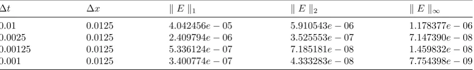
Table 4: TheL1, L2 andL∞ errors calculated by MLRPI for Example3.2 with different ∆xand ∆tat time
t= 1.0.
∆t ∆x ∥E∥1 ∥E∥2 ∥E∥∞
0.01 0.0125 4.042456e−05 5.910543e−06 1.178377e−06
0.0025 0.0125 2.409794e−06 3.525553e−07 7.147390e−08
0.00125 0.0125 5.336124e−07 7.185181e−08 1.459832e−08
0.001 0.0125 3.400774e−07 4.333283e−08 7.754398e−09
located points on the boundary and domain of the problem i.e. interval [0 1] so that the dis-tance between two consecutive nodes in each di-rection is constant and equal toh. Assuming that u(xi, k∆t), i = 1,2, ..., N are known, our aim is to compute u(xi,(k+ 1)∆t), i = 1,2, ..., N. So, we have N unknowns and to compute these
(2.36) to have
1 ∆t2
∑N j=1
(∫ Ωi
qϕj(x)dx
) u(jk+1)
+
(
1 ∆t+
1 3 )∑ N j=1 (∫ Ωi qx 2ϕ
j(x)dx
) u(jk+1)
−1
3
∑N j=1
( ∂ϕj(x)
∂x
x=xi+rq −
∂ϕj(x)
∂x
x=xi−rq
) u(jk+1)
−1
3
∑N j=1
(
x∂ϕj(x) ∂x
x=xi+rq
−x∂ϕj(x) ∂x
x=xi−rq
) u(jk+1)
+1 3
∑N j=1
( ϕj(x)
x=xi+rq
−ϕj(x)
x=xi−rq
) u(jk+1)
= 2 ∆t2
∑N j=1
(∫ Ωi
qϕj(x)dx
) u(jk)
−1 3 ∑N j=1 (∫ Ωi qx 2ϕ
j(x)dx
) u(jk)
+1 3
∑N j=1
( ∂ϕj(x)
∂x
x=xi+rq
−∂ϕj(x)
∂x
x=xi−rq
) u(jk)
+1 3
∑N j=1
(
x∂ϕj(x) ∂x
x=xi+rq
−x∂ϕj(x) ∂x
x=xi−rq
) u(jk)
−1
3
∑N j=1
( ϕj(x)
x=xi+rq
−ϕj(x)
x=xi−rq
) u(jk)−
1 ∆t2
∑N j=1
(∫ Ωi
qϕj(x)dx
) u(jk−1)
+
(
1 ∆t−
1 3 )∑ N j=1 (∫ Ωi qx 2ϕ
j(x)dx
) u(jk−1)
+1 3
∑N j=1
( ∂ϕj(x)
∂x
x=xi+rq −
∂ϕj(x)
∂x
x=xi−rq
) u(jk−1)
+1 3
∑N j=1
(
x∂ϕj(x) ∂x
x=xi+rq
−x∂ϕj(x) ∂x
x=xi−rq
) u(jk−1)
−1
3
∑N j=1
( ϕj(x)
x=xi+rq −
ϕj(x) x=xi−rq
)
u(jk−1)+
1 3 ∫ Ωi q (
g(k+1)(x) +g(k)(x) +g(k−1)(x))dx.
(2.37)
2.5 Implementation
For the boundary points, we have
∀k:uk(x1) =φ0(k), uk(xN) =φ1(k),
xi ∈∂Ω ={x1= 0, xN = 1}.
of the problem are given below:
[ 1 ∆t2
∑N
j=1Ai,j+ ( 1
∆t+
1 3
) ∑N j=1Bi,j
−1 3
∑N
j=1Ci,j− 1 3
∑N
j=1Di,j+ 1 3
∑N j=1Ei,j
]
u(jk+1) =
[ 2 ∆t2
∑N
j=1Ai,j−13
∑N
j=1Bi,j+
1 3
∑N
j=1Ci,j+13 ∑N
j=1Di,j−13 ∑N
j=1Ei,j ]
u(jk)+
[
− 1 ∆t2
∑N
j=1Ai,j+ ( 1
∆t−
1 3
) ∑N j=1Bi,j
+13∑Nj=1Ci,j+13
∑N
j=1Di,j−13
∑N j=1Ei,j
]
u(jk−1)+Fi(k−1, k, k+ 1),
(2.39) where
Ai,j =
∫ Ωi
qϕj(x)dx,
Bi,j =
∫ Ωi
qx
2ϕ
j(x)dx,
Ci,j =
(
∂ϕj(x)
∂x
x=xi+rq
−∂ϕj(x)
∂x
x=xi−rq
) ,
Di,j =
(
x∂ϕj(x) ∂x
x=xi+rq
−x∂ϕj(x) ∂x
x=xi−rq
) ,
Ei,j =
( ϕj(x)
x=xi+rq
− ϕj(x) x=xi−rq
) ,
Fi(k−1, k, k+ 1) = 1 3 ∫ Ωi q (
g(k+1)(x) +g(k)(x) +g(k−1)(x))dx.
(2.40) Assuming
Ai,j = ∆1t2Ai,j+
( 1 ∆t+
1 3 )
Bi,j
−1 3Ci,j−
1 3Di,j+
1 3Ei,j,
Bi,j = ∆2t2Ai,j−13Bi,j+13Ci,j+
1 3Di,j−
1 3Ei,j,
(2.41)
Ci,j =−∆1t2Ai,j+
( 1 ∆t−
1 3 )
Bi,j+
1 3Ci,j +
1 3Di,j−
1 3Ei,j,
Fk= [F1(k−1, k, k+ 1),
F2(k−1, k, k+ 1), ..., FN(k−1, k, k+ 1)]T ,
U = [u1, u2, ..., uN]T,
yeilds
AU(k+1) =BU(k)+CU(k−1)+Fk. (2.42)
Furthermore, to satisfy Eqs. (2.38), for both nodes belong to the boundary, i.e., {x1, xN}, we set
∀k:Fki =φi(k),∀j :Bi,j =Ci,j = 0,
Ai,j =
{
1, i=j,
0, i̸=j. (2.43)
At the first time level, when k= 0, according to the initial conditions that were introduced in Eq. (1.2), we apply the following assumptions:
u(0) =g1(x),
and
u(−1)∼=u(1)−2∆tg2(x),
where g1(x) = [g1(x1), g1(x2), ..., g1(xN)]T and
g2(x) = [g2(x1), g2(x2), ..., g2(xN)]T.
3
Numerical demonstrations
This size is significant enough to have sufficient number of nodes (n) to give appropriate shape functions. Also, in Eq. (2.10), we setm= 5.
Example 3.1 Consider the telegraph equation (1) with variable coefficients α = x2, β =x and
A = 1 +x over the domain [0 , 1] with the fol-lowing initial and boundary conditions:
u(x,0) = 0, ∂u
∂t(x,0) = 0,
u(0, t) = 0, u(1, t) = 0, t≥0.
The exact solution is given by
u(x, t) =t3x2(1−x)2, (x, t)∈[0,1]×[0,1]
and
g(x, t) = (6t+ 6x2t2+x2t3)x2(1−x)2
−t3(1 +x)(2−12x+ 12x2).
The results of the example are reported in Tables
1, 2 and 3 and Fig f1. As it is seen, MLRPI method is of high accuracy. Also Tables 1 and 2 show the order of convergence of the scheme. It can be seen that the errors are decreasing as we decrease ∆t or ∆x.]
0 0.1 0.2 0.3 0.4 0.5 0.6 0.7 0.8 0.9 1 0
0.01 0.02 0.03 0.04 0.05 0.06 0.07
x
u(x,t)
Exact solution Numerical solution
Figure 1: Numerical solutions and exact solution at time t = 1.0 for Example 3.1. The solid line corresponds to the exact solution, the stared line corresponds to numerical solution of the MLRPI with ∆t= 0.001 and ∆x= 0.0125.
Example 3.2 In this example, telegraph equa-tion (1) is considered with variable coefficients
α=x2,β=xandA= 1+xover the domain [0 , 1] and following initial and boundary conditions:
u(x,0) = 0, ∂u
∂t(x,0) = 0,
u(0, t) = 0, u(1, t) = 0, t≥0.
The exact solution is given by
u(x, t) =t2(1−x)sinh(x), (x, t)∈[0,1]×[0,1]
and
g(x, t) = (2 + 4x2t+x2t2−t2−xt2)×
(1−x)sinh(x) + (2t2+ 2xt2)cosh(x).
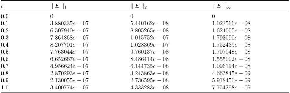
The results of the example are reported in Ta-bles 4,5 and 6 and Fig2. As it is seen, MLRPI method is of high accuracy. Also Tables 4 and 5 show the order of convergence of the scheme. It can be seen again the errors are decreasing as we decrease ∆tor ∆x.
0 0.1 0.2 0.3 0.4 0.5 0.6 0.7 0.8 0.9 1 0
0.05 0.1 0.15 0.2 0.25 0.3 0.35
x
u(x,t)
Exact solution
Numerical solution
Figure 2: Numerical solutions and exact solution at time t = 1.0 for Example 3.2. The solid line corresponds to the exact solution, the stared line corresponds to numerical solution of the MLRPI with ∆t= 0.001 and ∆x= 0.0125.
4
Conclusions
In this article, The meshless local radial point interpolation (MLRPI) method has been formu-lated and successfully implemented for solving the linear telegraph equation with variable coef-ficients. The time variable has been discretized by using finite differences approximation. Also, weak form of the discretized equations has been constructed on local subdomains. Furthermore, The radial point interpolation method is adopted for approximating the field variables. All integra-tions are regular, therefore the Gaussian quadra-ture rule used to calculate the numerical integra-tion for local weak form.
Table 5: TheL1, L2 andL∞ errors calculated by MLRPI for Example3.2 with different ∆xand ∆tat time
t= 1.0.
∆t ∆x ∥E∥1 ∥E∥2 ∥E∥∞
0.001 0.1 2.284578e−04 7.702824e−05 3.246693e−05
0.001 0.05 2.576054e−05 6.007151e−06 1.877456e−06
0.001 0.025 2.893497e−06 4.757451e−07 1.179273e−07
0.001 0.0125 3.400774e−07 4.333283e−08 7.754398e−09
Table 6: TheL1, L2 andL∞ errors calculated by MLRPI for Example 2 with differenttat ∆x= 0.0125 and
∆t= 0.001.
t ∥E∥1 ∥E∥2 ∥E∥∞
0.0 0 0 0
0.1 3.880335e−07 5.440162e−08 1.023566e−08
0.2 6.507940e−07 8.805265e−08 1.624005e−08
0.3 7.864868e−07 1.015752e−07 1.793090e−08
0.4 8.207701e−07 1.028369e−07 1.752439e−08
0.5 7.763044e−07 9.760137e−08 1.707048e−08
0.6 6.652667e−07 8.486414e−08 1.555002e−08
0.7 4.956624e−07 6.144735e−08 1.096194e−08
0.8 2.870293e−07 3.243863e−08 4.663845e−09
0.9 2.130055e−07 2.736595e−08 5.918456e−09
1.0 3.400774e−07 4.333283e−08 7.754398e−09
which requires neither domain elements nor back-ground cells in either the interpolation or the in-tegration. The main advantage of the scheme is to capture the behaviour of solution for similar problems with variable coefficients where most of the schemes fail. Test problems verified the accu-racy and convergency of the proposed approach.
References
[1] S. Abbasbandy, HR. Ghehsareh, I Hashim, Ameshfree method for the solution of two-dimensional cubic nonlinear Schr¨odinger equation,Engineering Analysis with Bound-ary Elements 37 (2013) 885-898.
[2] S. Abbasbandy, HR. Ghehsareh, I Hashim, Numerical analysis of a mathematical model for capillary formation in tumor angiogen-esis using ameshfree method based on the radial basis function, Engineering Analysis with Boundary Elements 36 (2012) 1811-1818.
[3] P. Almenar, L. Jodar, J.A. Martin, Mixed problems for the time-dependent telegraph equation: Continuous numerical solutions with a priori error bounds, Math. Comput. Modelling 25 (1997) 31-44.
[4] R. Aloy, M. C. Casabn, L.A. Caudillo-Mata, L. Jdar, Computing the variable coefficient telegraph equation using a discrete eigen-function method, Comput. Math. Appl. 54 (2007) 448-458.
[5] M. Aslefallah, E. Shivanian, E. Nonlin-ear fractional integro-differential reaction-diffusion equation via radial basis functions, The European Physical Journal Plus 130 (2015) 1-9.
[6] J. Banasiak, J. R. Mika, Singularly per-turbed telegraph equations with applications in the random walk theory, J. Appl. Math. Stoch. Anal. 11 (1998) 9-28.
[8] T. Belytschko, Y. Y. Lu, L. Gu, Element-free Galerkin methods.International Journal for Numerical Methods in Engineering37 (1994) 229-256.
[9] T. Belytschko, Y. Y. Lu, L. Gu, Element free Galerkin methods for static and dynamic fracture,International Journal of Solids and Structures 32 (1995) 2547-2570.
[10] W. E. Boyce, R. C. DiPrima, Differential Equations Elementary and Boundary Value Problems, Wiley, New York, 1977.
[11] M. Ciment, S.H. Leventhal, A note on the operator compact implicit method for the wave equation,Math. Comp. 32 (1978) 143-147.
[12] M. Ciment, S. H. Leventhal, Higher order compact implicit schemes for the wave equa-tion,Math. Comp.29 (1975) 985-994.
[13] G. Dahlquist, On accuracy and uncondi-tional stability of linear multi-step methods for second order differential equations, BIT 18 (1978) 133-136.
[14] M. Dehghan, A. Mohebbi, High order im-plicit collocation method for the solution of two-dimensional linear hyperbolic equation, Numer. Methods PDEs 25 (2009) 232-243.
[15] M. Dehghan, A. Shokri, A numerical method for solution of the two dimensional sine-Gordon equation using the radial basis func-tions, Mathematics and Computers inSimu-lation 79 (2008) 700-715.
[16] M. Dehghan, A. Shokri, A numerical method for solving the hyperbolic telegraph equa-tion,Numer. Methods PDEs 24 (2008) 1080-1093.
[17] H. Ding, Y. Zhang, A new fourth-order com-pact finite difference scheme for the two-dimensional second-order hyperbolic equa-tion,J. Comp. Appl. Math. 230 (2009) 626-632.
[18] M. S. El-Azab, M. El-Gamel, A numerical algorithm for the solution of telegraph equa-tions, Appl. Math. Comput.190 (2007) 757-764.
[19] C. Franke, R. Schaback, Solving partial dif-ferential equations by collocation using ra-dial basis functions, Applied Mathematics and Computation 93 (1997) 73-82.
[20] Z. J. Fu, W. Chen, L. Ling. Method of ap-proximate particular solutions for constant-and variable-order fractional diffusion mod-els, Eng. Anal. Boundary Elem. 57 (2015) 37-46.
[21] Z. J. Fu, W. Chen, H.T. Yang. Bound-ary particle method for Laplace transformed time fractional diffusion equations, Journal of Computational Physics 235 (2013) 52-66.
[22] VR. Hosseini, E. Shivanian, W. Chen, Local integration of 2-D fractional telegraph equa-tion via local radial point interpolant ap-proximation,The European Physical Journal Plus 130 (2015) 1-21.
[23] D. Hu, S. Long, K. Liu, G. Li, A modi-fied meshless local Petrov-Galerkin method to elasticity problems in computer modeling and simulation, Engineering Analysis with Boundary Elements 30 (2006) 399-404.
[24] L. Jdar, D. Goberna, Analytic-numerical so-lution with a priori error bounds for cou-pled time-dependent telegraph equations: Mixed problems, Math Comput. Modelling 30 (1999) 39-53.
[25] P. M. Jordan, A. Puri, Digital signal prop-agation in dispersive media, J. Appl. Phys. 85 (1999) 1273-1282.
[26] E. Kansa, Multiquadrics-a scattered data approximation scheme with applications to computational fluid-dynamics. I. Surface ap-proximations and partial derivative esti-mates Computers & Mathematics with Ap-plications 19 (1990) 127-145.
[27] S. F. Li, W. K. Liu, Meshfree and particle methods and their application,Applied Me-chanics Reviews 55 (2002) 1-34.
[29] J. Lin, W. Chen, K. Y. Sze, A new radial basis function for Helmholtz problems, En-gineering Analysis with Boundary Elements 36 (2012) 1923-1930.
[30] K. Liu, S. Long, G. Li, A simple and less-costly meshless local Petrov-Galerkin (MLPG) method for the dynamic fracture problem, Engineering Analysis with Bound-ary Elements 30 (2006) 72-76.
[31] R. K. Mohanty, An unconditionally sta-ble difference scheme for the one-space di-mensional linear hyperbolic equation, Appl. Math. Lett.17 (2004) 101-105.
[32] R. K. Mohanty, M. K. Jain, An uncondi-tionally stable alternating direction implicit scheme for the two space dimensional linear hyperbolic equation,Numer. Methods PDEs 17 (2001) 684-688.
[33] R. K. Mohanty, M. K. Jain, U. Arora, An unconditionally stable ADI method for the linear hyperbolic equation in three space di-mensions, Int. J. Comput. Math. 79 (2002) 133-142.
[34] R. K. Mohanty, M. K. Jain, K. George, High order difference schemes for the system of two space second order nonlinear hyper-bolic equations with variable coefficients, J. Comp. Appl. Math. 70 (1996) 231-243.
[35] R. K. Mohanty, M. K. Jain, K. George, On the use of high order difference methods for the system of one space second order non-linear hyperbolic equations with variable co-efficients, J. Comp. Appl. Math. 72 (1996) 421-431.
[36] M. J. D. Powell, Theory of radial basis func-tion approximafunc-tion in 1990, in: F.W. Light (Ed.),Adv. Numer. Anal. (1992) 303-322.
[37] M. Sharan, E. J. Kansa, S. Gupta, Appli-cation of the multiquadric method for nu-merical solution of elliptic partial differential equations, Appl. Math. Comput. 84 (1997) 275-302.
[38] A. Shirzadi, L. Ling, S. Abbasbandy, Mesh-lesss imulations of the two-dimensional
fractional-time convection-diffusion-reaction equations, Engineering Analysis with Boundary Elements 36 (2012) 1522-1527.
[39] A. Shirzadi, V. Sladek, J. Sladek, A local in-tegral equation formulation to solve coupled nonlinear reaction-diffusion equations by us-ing movus-ing least square approximation, En-gineering Analysis with Boundary Elements 37 (2013) 8-14.
[40] E. Shivanian, A new spectral meshless ra-dial point interpolation (SMRPI)method: a well-behaved alternative to themeshlessweak forms, Engineering Analysis with Boundary Elements 54 (2015) 1-12.
[41] E. Shivanian, S. Abbasbandy, MS. Al-huthali, HH. Alsulami, Local integration of 2-D fractional telegraph equation via mov-ing least squares approximation, Engineer-ing Analysis with Boundary Elements 56 (2015) 98-105.
[42] E. Shivanian, Analysis of meshless local ra-dial point interpolation (MLRPI) on a non-linear partial integro-differential equation arising in population dynamics,Engineering Analysis with Boundary Elements 37 (2013) 1693-1702.
[43] E. Shivanian, On the convergence analysis, stability, and implementation of meshless lo-cal radial point interpolation on a class of three-dimensional wave equations, Interna-tional Journal for NumericalMethods in En-gineering (in press) 2015. http://dx.doi. org/10.1002/nme.4960./
[44] E. Shivanian, HR. Khodabandehlo, Meshless local radial point interpolation (MLRPI) on the telegraph equation with purely integral conditions, European Physical Journal 129 (2014) 241-251.
[45] A. N. Tikhonov, A. A. Samarskii, Equations of Mathematical Physics, Dover, New York, 1990.
[47] H. Wendland, Error estimates for interpo-lation by compactly supported radial basis functions of minimal degree, Journal of Ap-proximation Theory 93 (1998) 258-396.
[48] V. H. Weston, S. He, Wave splitting of the telegraph equation in R3 and its applica-tion to inverse scattering,Inverse Problems, 9 (1993) 789-812.
Dr. Elyas Shivanian was born in Zanjan province, Iran in August 26, 1982. He started his mas-ter course in applied mathemat-ics in 2005 at Amirkabir Univer-sity of Technology and has finished MSc. thesis in the field of fuzzy linear programming in 2007. His research in-terests are analytical and numerical solutions of ODEs, PDEs and IEs. He has published sev-eral papers on these subjects. He also has pub-lished some papers in other fields, for more infor-mation see pleasehttp://scholar.google.com/ citations?user=MFncks8AAAAJ&hl=en
Saeid Abbasbandy has got PhD de-gree from Kharazmi University in 1996 and now he is the full pro-fessor in Imam Khomeini Interna-tional University, Ghazvin, Iran. He has published more than 300 papers in international journals and conferences. Now, he is working on numerical analysis and fuzzy numerical analysis.