HAAR BASIS METHOD TO SOLVE SOME INVERSE PROBLEMS FOR TWO-DIMENSIONAL PARABOLIC AND HYPERBOLIC EQUATIONS

(1)

HAAR BASIS METHOD TO SOLVE SOME INVERSE PROBLEMS FOR TWO-DIMENSIONAL PARABOLIC AND HYPERBOLIC

EQUATIONS

R. POURGHOLI1_{, S. FOADIAN}1_{, A. ESFAHANI}1 _§

Abstract. A numerical method consists of combining Haar basis method and Tikhonov

regularization method. We apply the method to solve some inverse problems for two-dimensional parabolic and hyperbolic equations using noisy data. In this paper, a stable numerical solution of these problems is presented. This method uses a sensor located at a point inside the body and measures theu(x, y, t) at a pointx=a,0< a <1. We also show that the rate of convergence of the method is as exponential. Numerical results show that a good estimation on the unknown functions of the inverse problems can be obtained within a couple of minutes CPU time at Pentium IV-2.53 GHz PC.

Keywords: Inverse problems, Haar basis method; Error analysis, Tikhonov regularization method, Noisy data.

AMS Subject Classiﬁcation: 65M32, 35K05, 35L02, 65T60.

Inverse problems are applied in many important scientific and technological fields. Hence, analysis, design implementation and testing of inverse algorithms are also the great scientific and technological interest.

The inverse heat conduction problem in a one-dimensional composite slab with rate-dependent pyrolysis chemical reaction and outgassing ﬂow eﬀects is investigated using the iterative regularization approach. The thermal properties of the composites are considered to be temperature-dependent, [32].

Cheng-Hung Huanga, Chun-Ying Yeha, and Helcio R.B. Orlande presented an itera-tive regularization method based on an inverse algorithm. The algorithm is applied to simultaneously determine the unknown temperature, concentration-dependent heat, and mass production rates for a chemically reacting ﬂuid. This work is done using interior measurements of temperature and concentration [17].

Kim et al. [27] solved an inverse heat conduction problem to estimate the surface temperature from temperature readings. Su and Neto [28] solved a two-dimensional inverse heat conduction problem to estimate the radial and circumferential transient dependence of the strength of a volumetric heat source in a cylindrical rod. Huang and Tsai [16] solved a three-dimensional inverse heat conduction problem to estimate the local time-dependent surface heat transfer coeﬃcients for plate ﬁnned-tube heat exchangers.

However, only few works have been done on the two-dimensional problems because of the complicated interaction and reﬂection of the thermal wave [9, 8]. Yang Ching-yu,

1

School of Mathematics and Computer Science, Damghan University, P.O.Box 36715-364, Damghan, Iran,

e-mail: [email protected], [email protected] and [email protected] § Manuscript received October 01, 2012.

(2)

[9] developed the two-dimensional hyperbolic heat conduction equations in an arbitrary body-ﬁtted coordinate grid and used non-oscillatory numerical schemes to approach the problem. Chen and Lin [8] formulated a numerical scheme involving the Laplace transform technique and the control volume method for the problem.

Mathematically, the inverse problems belong to the class of problems called the ill-posed problems, i.e. small errors in the measured data can lead to large deviations in the estimated quantities. As a consequence, their solution does not satisfy the general requirement of existence, uniqueness, and stability under small changes to the input data. To overcome such difficulties, a variety of techniques for solving inverse problems have been proposed [32]-[29] and among the various methods such as: Tikhonov regularization [31], iterative regularization [2], mollification [22], BFM (Base Function Method) [25], SFDM (Semi Finite Difference Method) [21], and the FSM (Function Specification Method ) [3]. Beck et al. [3] compared the FSM, the Tikhonov regularization and the iterative reg-ularization, using experimental data. Beck and Murio [5] presented a new method that combines the function specification method of Beck with the regularization technique of Tikhonov. Murio and Paloschi [23] proposed a combined procedure based on a data fil-tering interpretation of the mollification method and FSM.

Haar functions have been used from 1910 when they were introduced by the Hungarian mathematician Haar [12]. The Haar transform is one of the earliest of what is known now as a compact, dyadic, orthonormal wavelet transform. The Haar function, being an odd rectangular pulse pair, is the simplest and oldest orthonormal wavelet with compact support. In the mean time, several deﬁnitions of the Haar functions and various general-izations have been published and used. They were intended to adopt this concept to some practical applications as well as to extend its in applications to diﬀerent classes of signals. Haar functions appear very attractive in many applications as for example, image coding, edge extraction and binary logic design.

Recently, Haar wavelets, [14], have been applied extensively for signal processing in communications and physics research, and have proved to be a wonderful mathematical tool. After discretizing the differential equations in a conventional way like the finite difference approximation, wavelets can be used for algebraic manipulations in the system of equations obtained which lead to better condition number of the resulting system.

The previous work, [14], in the system analysis via Haar wavelets was led by Chen and Hsiao [7], who first derived a Haar operational matrix for the integrals of the Haar functions vector and put the application for the Haar analysis into the dynamical systems. Then, the pioneer work in state analysis of linear time delayed systems via Haar wavelets was laid down by Hsiao [15], who first proposed a Haar product matrix and a coefficient matrix. Hsiao and Wang proposed a key idea to transform the time-varying function and its product with states into a Haar product matrix. Kalpana and Raja Balachandar [18] presented Haar wavelet based method of analysis for observer design in the generalized state space or singular system of transistor circuits.

In this paper, a numerical method is presented based on Haar wavelet method and 0th, 1st, and 2nd Tikhonov regularization.

(3)

1. Mathematical formulation

Definition 1.1. The Haar wavelet family for x∈[0,1)is deﬁned as follows, [14],

hi(x) =

    

1, x∈[_mk,k+0.5_m ), −1, x∈[k+0.5_m ,k+1_m ), 0, elsewhere.

(1.1)

integer m= 2j,(j= 0,1, . . . , J) indicates the level of the wavelet;

k = 0,1, . . . , m−1 is the translation parameter. Maximal level of resolution is J. The indexi is calculated according the formula i=m+k+ 1, such that

∫ 1

0

hi(x)hl(x) dx=

1 2j δil, where δil is Kronecker delta.

In the case of minimal values m = 1, k = 0 we have i = 2, the maximal value of i

is i= 2J+1 = M. It is assumed that the value i = 1 corresponds to the scaling function for which h1 ≡ 1 in [0,1). let us defined collocation points xl = l−_M0.5,(l = 1,2, . . . , M) and discretis the Haar functionhi(x); in this way we get the coefficient matrix H and the operational matrices of integrationP, Q, which are M square matrices, are defined by the equations

(H)il = (hi(xl)), (1.2)

(P H)il =

∫ xl

0

hi(x)dx, (1.3)

(QH)il =

∫ xl

0

∫ x

0

hi(s)ds dx. (1.4)

The elements of the matrices H, P and Q can be evaluted according to (1.2), (1.3) and

(1.4). For example when M = 2,4 we have,

H2 =

(

1 1

1 −1

) , P2 =

1 4 ( 2 −1 1 0 ) , Q2=

1 32

(

5 −4

4 −3

) ,

H4 =

   

1 1 1 1

1 1 −1 −1

1 −1 0 0

0 0 1 −1

  

, P4 =

1 16    

8 −4 −2 −2

4 0 −2 2

1 1 0 0

1 −1 0 0

  

,

Q4 =

1 128    

21 −16 −4 −12

16 −11 −4 −4

6 −2 −3 0

2 −2 0 −3

  

.

Remark 1.1. Any function Υ∈L2([0,1)×[0,1)) can be decomposed as

Υ(x, y) =

∞ ∑ l=1 ∞ ∑ i=1

cilhi(x)hl(y),

where the coeﬃcientscil are determined by

cil= 2j1+j2

∫ 1

0

∫ 1

0

Υ(x, y)hi(x)hl(y)dxdy,

where

i= 2j1 ₊_k

(4)

The series expansion ofΥ(x, y)contains an inﬁnite terms. IfΥ(x, y)is piecewise constant by itself, or may be approximated as piecewise constant during each subinterval, then

Υ(x, y) will be terminated at ﬁnite terms, that is,

Υ(x, y) =

M2

∑

l=1 M1

∑

i=1

cilhi(x)hl(y) =HM1T (x)CM1×M2HM2(y),

where the coeﬃcients CM1×M2 and the Haar functions vectors HMT1(x) and HM2(y) are deﬁned as,

H_MT₁(x) =(h1(x) h2(x) . . . hM1(x)

) ,

HM2(y) =

(

h1(y) h2(y) . . . hM2(y)

)T

,

CM1×M2=

    

c11 c12 . . . c1(M2)

c21 c22 . . . c2(M2)

..

. ... ...

c(M1)1 c(M1)2 . . . c(M1)(M2)

   

.

Where′T′ means transpose and M1 = 2J1+1_{, M}_{2 = 2}J2+1_.

1.1. Inverse Problem for the Two-Dimensional Heat Equation. In this section, we consider the following inverse parabolic problem in the two-dimensionlal form

ut=uxx+uyy, 0< x <1, 0< y <1, 0< t < tf, (1.5a)

u(x, y,0) =f(x, y), 0≤x≤1, 0≤y≤1, (1.5b)

u(0, y, t) =g(y, t), 0≤y≤1, 0≤t≤tf, (1.5c)

u(1, y, t) =h(y, t), 0≤y≤1, 0≤t≤tf, (1.5d)

u(x,0, t) =p(x, t), 0≤x≤1, 0≤t≤tf, (1.5e)

u(x,1, t) =q(x, t), 0≤x≤1, 0≤t≤tf, (1.5f)

and the overspeciﬁed condition

u(a, y, t) =ϕ(y, t), 0≤y≤1 0≤t≤tf, (1.5g)

where 0< a < 1 is a ﬁxed point, f(x, y) is a continuous known function, h(y, t), p(x, t),

q(x, t) and ϕ(y, t) are infinitely differentiable known functions and tf represents the final

time of interest for the time evolution of the problem; while function g(y, t) is unknown

which should be determined from some interior temperature measurements.

Now, let us divide the interval [0, tf] intoN equal parts of length ∆t=

tf

N and denote

ts = (s−1)∆t, s = 1,2, ..., N. We assume that ˙u′′◦◦ can be expanded in terms of Haar

basis as,

˙

u′′◦◦(x, y, t) =

M2

∑

j=1 M1

∑

i=1

cs(ij)hi(x)hj(y) =HM1T (x)CM1×M2HM2(y) (1.6)

where ., ′ and ◦ mean diﬀerentiation with respect to t, x and y respectively. the vector

(5)

Integrating equation (1.6) twice with respect to x from ato x and twice with respect

toy from 0 toy we obtain,

˙

u◦◦(x, y, t) = ˙u◦◦(a, y, t) + (x−a) ˙u′◦◦(a, y, t) + [(QM1HM1)T(x)

−(QM1HM1)T(a)−(x−a)(PM1HM1)T(a)]CM1×M2HM2(y), (1.7)

˙

u′′(x, y, t) = ˙u′′(x,0, t) +yu˙′′◦(x,0, t) +H_MT₁(x)CM1×M2(QM2HM2)(y), (1.8)

By the boundary conditions, we obtain,

˙

u◦◦(a, y, t) = ˙ϕ◦◦(y, t), u˙◦◦(1, y, t) = ˙h◦◦(y, t),

˙

u′′(x,0, t) = ˙p′′(x, t), u˙′′(x,1, t) = ˙q′′(x, t).

Puttingx= 1 in equation (1.7) andy = 1 in equation (1.8), we obtain,

˙

u′◦◦(a, y, t) = 1

1−ah˙

◦◦₍_{y, t}₎₋ 1

1−aϕ˙

◦◦₍_{y, t}_{) + [} 1

1−a(QM1HM1)

T₍_a₎

− 1

1−a(QM1HM1)

T_{(1) + (}_P

M1HM1)T(a)]CM1×M2HM2(y), (1.9)

˙

u′′◦(x,0, t) = ˙q′′(x, t)−p˙′′(x, t)−H_M1T (x)CM1×M2(QM2HM2)(1). (1.10)

Substituting equations (1.9) and (1.10) into equations (1.7) and (1.8), we obtain,

˙

u◦◦(x, y, t) = 1−x

1−a

˙

ϕ◦◦(y, t) + x−a

1−a

˙

h◦◦(y, t) + [(QM1HM1)T(x)

−x−a

1−a(QM1HM1)

T_{(1) +}x−1

1−a(QM1HM1)

T₍_a_)]_C

M1×M2HM2(y), (1.11)

˙

u′′(x, y, t) = (1−y) ˙p′′(x, t) +yq˙′′◦(x, t)

+H_M1T (x)CM1×M2[(QM2HM2)(y)−y(QM2HM2)(1)]. (1.12)

Integrating equations (1.11) and (1.12) with respect totfromtstotand twice with respect

toy from 0 toy from equation (1.11) we obtain,

u′′(x, y, t) = (t−ts)HM1T (x)CM1×M2[(QM2HM2)(y)−y(PM2F2)] +u′′(x, y, ts)

+y[q′′(x, t)−q′′(x, ts)] + (1−y)[p′′(x, t)−p′′(x, ts)], (1.13)

u◦◦(x, y, t) =u◦◦(x, y, ts) +

1−x

1−a[ϕ

◦◦₍_{y, t}₎₋_ϕ◦◦₍_{y, t} s)]

+x−a

1−a[h

◦◦₍_{y, t}₎₋_h◦◦₍_{y, t}

s)] + (t−ts)[(QM1HM1)T(x)

−x−a

1−a(PM1F1)

T ₊x−1

1−a(QM1HM1)

T₍_a_)]_C

M1×M2HM2(y), (1.14)

˙

u(x, y, t) = [(QM1HM1)T(x)−

x−a

1−a(PM1F1)

T ₊x−1

1−a(QM1HM1)

T₍_a_)]_C M1×M2

[(QM2HM2)(y)−y(PM2F2)]

+x−a

1−a[ ˙h(y, t)−y ˙

h(1, t) + (y−1) ˙h(0, t)]

+1−x

1−a[ ˙ϕ(y, t)−yϕ˙(1, t) + (y−1) ˙ϕ(0, t)]

+(1−y) ˙p(x, t) +yq˙(x, t), (1.15)

u(x, y, t) = (t−ts)[(QM1HM1)T(x)−

x−a

1−a(PM1F1)

T ₊x−1

1−a(QM1HM1)

T₍_a_)]

CM1×M2[(QM2HM2)(y)−y(PM2F2)]

+1−x

(6)

+x−a

1−a[h(y, t)−h(y, ts)−y{h(1, t)−h(1, ts)}+ (y−1){h(0, t)−h(0, ts)}]

+u(x, y, ts) + (1−y)[p(x, t)−p(x, ts)] +y[q(x, t)−q(x, ts)]. (1.16)

Discretizising the results by assuming x→xl, y →yk, t→ts+1 we obtain,

u′′(xl, yk, ts+1) = (ts+1−ts)HMT1(xl)CM1×M2[(QM2HM2)(yk)−yk(PM2F2)]

+u′′(xl, yk, ts) +yk[q′′(xl, ts+1)−q′′(xl, ts)]

+(1−yk)[p′′(xl, ts+1)−p′′(xl, ts)], (1.17)

u◦◦(xl, yk, ts+1) =u◦◦(xl, yk, ts) +

1−xl

1−a[ϕ

◦◦₍_y

k, ts+1)−ϕ◦◦(yk, ts)]

+xl−a

1−a[h

◦◦₍_y

k, ts+1)−h◦◦(yk, ts)] + (ts+1−ts)[(QM1HM1)T(xl)

−xl−a

1−a(PM1F1)

T ₊xl−1

1−a(QM1HM1)

T₍_a_)]_C

M1×M2HM2(yk), (1.18)

˙

u(xl, yk, ts+1) = [(QM1HM1)T(xl)−

xl−a

1−a(PM1F1)

T ₊xl−1

1−a(QM1HM1)

T₍_a_)]

CM1×M2[(QM2HM2)(yk)−yk(PM2F2)]

+xl−a

1−a[ ˙h(yk, ts+1)−yk ˙

h(1, ts+1) + (yk−1) ˙h(0, ts+1)]

+1−xl

1−a[ ˙ϕ(yk, ts+1)−yk ˙

ϕ(1, ts+1) + (yk−1) ˙ϕ(0, ts+1)]

+(1−yk) ˙p(xl, ts+1) +ykq˙(xl, ts+1), (1.19)

u(xl, yk, ts+1) = (ts+1−ts)[(QM1HM1)T(xl)−

xl−a

1−a(PM1F1)

T

+xl−1

1−a(QM1HM1)

T₍_a_)]_C

M1×M2[(QM2HM2)(yk)−yk(PM2F2)]

+1−xl

1−a[ϕ(yk, ts+1)−ϕ(yk, ts)−yk{ϕ(1, ts+1)−ϕ(1, ts)} +(yk−1){ϕ(0, ts+1)−ϕ(0, ts)}] +

xl−a

1−a[h(yk, ts+1)−h(yk, ts)

−yk{h(1, ts+1)−h(1, ts)}+ (yk−1){h(0, ts+1)−h(0, ts)}]

+u(xl, yk, ts) + (1−yk)[p(xl, ts+1)−p(xl, ts)] +yk[q(xl, ts+1)−q(xl, ts)], (1.20)

where vectorsF1 andF2 are deﬁned as

F1 = [1,0_{| {z }}, . . . ,0

(M1−1)

]T, F2= [1,0_{| {z }}, . . . ,0

(M2−1)

]T,

andH, P, Q are obtained from equations (1.2), (1.3), (1.4). In the following scheme

˙

u(xl, yk, ts+1) =u′′(xl, yk, ts+1) +u◦◦(xl, yk, ts+1), (1.21)

which leads us from the time layerts tots+1 is used, where,

xl=

l−0.5

M1 , l= 1,2, . . . ,(M1 = 2

J1+1₎_,

yk=

k−0.5

M2 , k= 1,2, . . . ,(M2 = 2

J2+1₎_,

(7)

Substituting equations (1.17), (1.18), (1.19) into equation (1.21), we obtain

[(QM1HM1)T(xl)−

xl−a

1−a(PM1F1)

T ₊xl−1

1−a(QM1HM1)

T₍_a₎₋_{T H}T M1(xl)]

CM1×M2[(QM2HM2)(yk)−yk(PM2F2)]−T[(QM1HM1)T(xl)

−xl−a

1−a(PM1F1)

T ₊xl−1

1−a(QM1HM1)

T₍_a_)]_C

M1×M2HM2(yk)

= 1−xl

1−a[ϕ

◦◦₍_y

k, ts+1)−ϕ◦◦(yk, ts)−ϕ˙(yk, ts+1) +ykϕ˙(1, ts+1) + (1−yk) ˙ϕ(0, ts+1)]

+xl−a

1−a[h

◦◦₍_y

k, ts+1)−h◦◦(yk, ts)−h˙(yk, ts+1) +ykh˙(1, ts+1) + (1−yk) ˙h(0, ts+1)]

+yk[q′′(xl, ts+1)−q′′(xl, ts)−q˙(xl, ts+1)]

+(1−yk)[p′′(xl, ts+1)−p′′(xl, ts)−p˙(xl, ts+1)]

+u′′(xl, yk, ts) +u◦◦(xl, yk, ts). (1.22)

The wavelet coeﬃcientCM1×M2 can be calculated from the equation (1.22).

Thus the linear system corresponding to the wavelet coeﬃcient CM1×M2 can be

ex-pressed as

ΛΘ =B. (1.23)

The Matrix Λ is ill-conditioned. On the other hand, asϕ(y, t) is aﬀected by measurement

errors, the estimate of Θ by (1.23) will be unstable so that the Tikhonov regularization

method must be used to control this measurement errors. The Tikhonov regularized

solution [13, 19, 30, 31] to the system of linear algebraic equation (1.23) is given by

zα(Θ) =∥ΛΘ−B∥22+α∥R(s)Θ∥22.

On the case of the zeroth-, ﬁrst-, and second-order Tikhonov regularization method the

matrixR(s), fors= 0,1,2,is given by, see e.g. [20]:

R(0) =IM1×M1 ∈R

M1×M1_,

R(1) =       

−1 1 . . . 0 0 0

0 −1 1 . . . 0 0

..

. ... ... ... ... ...

0 0 . . . −1 1 0

0 0 . . . 0 −1 1

     

∈R

(M1−1)×M1_,

R(2) =       

1 −2 1 0 . . . 0 0

0 1 −2 1 0 . . . 0

..

. ... ... ... ... ... ...

0 0 . . . 1 −2 1 0

0 0 . . . 0 1 −2 1

     

∈R

(M1−2)×M1_,

whereM1= (γ+ 1)×(ι+ 1).

Therefore, we obtain the Tikhonov regularized solution of the regularized equation as

Θα=

[

ΛTΛ +α(R(s))TR(s)]−1ΛTB.

(8)

2. Error Analysis

In this section, the convergence of the Haar basis method is investigated for inverse problem with two-dimensional heat equation.

At the ﬁrst, suppose that ˙u′′◦◦(x, y, t) = Υ(x, y, t). We show that if Υ(x, y, t) is

continuous and it satisﬁes Lipschitz condition with respect to one of its variables and

M1 =M2 = 2J+1, then the method is convergence.

Now, assume that Υ(x, y, t) satisﬁes Lipschitz condition on [0,1]×[0,1], that is,

∃ L >0, ∀ (x, y1), (x, y2)∈[0,1]×[0,1] : |Υ(x, y1, t)−Υ(x, y2, t)| ≤L|y1−y2|. (2.1)

Also, suppose that Υ∗(x, y) is an approximation of Υ(x, y) as follows:

Υ∗(x, y, t) =

M2

∑

i2=1

M1

∑

i1=1

ci1i2hi1(x)hi2(y),

and

Υ∗(x, y, t) =

M

∑

i2=1

M

∑

i1=1

ci1i2hi1(x)hi2(y),

where the coeﬃcientsci1i2 are determined by

ci1i2 = 2

2j

∫ 1

0

∫ 1

0

Υ(x, y)hi1(x)hi2(y)dxdy,

where

i1=i2 = 2j +k+ 1, j>0,06k <2j.

Therefore, we can compute the error as follows:

e∗(x, y) = Υ(x, y, t)−Υ∗(x, y, t)

=

∞

∑

i2=M+1

∞

∑

i1=M+1

ci1i2hi1(x)hi2(y)

=

∞

∑

i1,i2=M+1

ci1i2hi1(x)hi2(y)

Hence,∥e∗∥2₂ is as:

∥e∗∥2₂ =

∫ 1

0

∫ 1

0

(

∞

∑

i1,i2=M+1

ci1i2hi1(x)hi2(y))

2_dxdy

=

∫ 1

0

∫ 1

0

(

∞

∑

i1,i2=M+1

ci1i2hi1(x)hi2(y)

∞

∑

l1,l2=M+1

cl1l2hl1(x)hl2(y))dxdy

=

∞

∑

i1,i2=M+1

∞

∑

l1,l2=M+1

ci1i2cl1l2(

∫ 1

0

∫ 1

0

hi1(x)hl1(x)hi2(y)hl2(y)dxdy)

=

∞

∑

i1,i2=M+1

(9)

Sinceci1i2 = 2

2j∫1 0

∫1

0 Υ(x, y, t)hi1(x)hi2(y)dxdy, according to (1.1), we can write

ci1i2 = 2

2j₍

∫ k+0.5

2j

k

2j

∫ k+0.5

2j

k

2j

Υ(x, y, t)dydx−

∫ k+0.5

2j

k

2j

∫ k+1

2j

k+0.5 2j

Υ(x, y, t)dydx

−

∫ k+1

2j

k+0.5 2j

∫ k+0.5

2j

k

2j

Υ(x, y, t)dydx+

∫ k+1

2j

k+0.5 2j

∫ k+1

2j

k+0.5 2j

Υ(x, y, t)dydx).

Now, using the mean value theorem, we can conclude

∃x1 ∈[

k 2j,

k+ 0.5

2j ], y1∈[

k 2j,

k+ 0.5 2j ], s.t.

∫ k+0.5

2j

k

2j

∫ k+0.5

2j

k

2j

Υ(x, y, t)dydx= 1

22j+2f(x1, y1, t),

∃x2 ∈[

k 2j,

k+ 0.5

2j ], y2∈[

k+ 0.5

2j ,

k+ 1 2j ], s.t.

∫ k+0.5

2j

k

2j

∫ k+1

2j

k+0.5 2j

Υ(x, y, t)dydx= 1

22j+2Υ(x2, y2, t),

∃x3 ∈[

k+ 0.5

2j ,

k+ 1

2j ], y3 ∈[

k 2j,

k+ 0.5 2j ], s.t.

∫ k+1

2j

k+0.5 2j

∫ k+0.5

2j

k

2j

Υ(x, y, t)dydx= 1

22j+2Υ(x3, y3, t),

∃x4 ∈[

k+ 0.5

2j ,

k+ 1

2j ], y4 ∈[

k+ 0.5

2j ,

k+ 1 2j ], s.t.

∫ k+1

2j k+0.5

2j

∫ k+1

2j k+0.5

2j

Υ(x, y, t)dydx= 1

22j+2Υ(x4, y4, t),

Thus, we can computeci1i2 as follows:

ci1i2 = 2

2j_[ 1

22j+2(Υ(x1, y1, t)−Υ(x2, y2, t)−Υ(x3, y3, t) + Υ(x4, y4, t))]

= 1

4[Υ(x1, y1, t)−Υ(x1, y2, t) + Υ(x1, y2, t)−Υ(x2, y2, t) −Υ(x3, y3, t) + Υ(x3, y4, t)−Υ(x3, y4, t) + Υ(x4, y4, t)]

≤ L

4[(y1−y2) + (x1−x2) + (y3−y4) + (x3−x4)]

≤ L

4[ 1

2j +

1

2j +

1

2j +

1 2j]

= (L

4)(

4

2j) =

(10)

The ﬁrst inequality is obtained with regard to relation (2.1). On the other hand, we have

∥e∗∥2₂ =

∞

∑

i1,i2=M+1

c2_i₁_i₂ 1 22j

≤ ∑∞

i1,i2=M+1

L2 22j

1 22j

=

∞

∑

i1,i2=M+1

L2 24j

=L2

∞

∑

i1,i2=M+1

1 24j

=L2

∞

∑

j=J+1 2j₋₁

∑

k=0

1 24j

=L2

∞

∑

j=J+1

2j−1 + 1

24j

=L2

∞

∑

j=J+1

1 23j

= 8

7L

2₍ 1

2J+1)

3

SinceM = 2J+1, we have

∥e∗∥2₂≤ 8

7L

2₍ 1

M)

3_,

and

∥e∗∥2≤

√ 8 7L(

1 M)

3 2.

Therefore, the Haar basis method will be convergent, i.e.

lim

J→∞e ∗_{= 0}

Moreover, the convergence is of order exponential, that is,

∥e∗∥2=O(

1

2J+1)

3

2 =O( 1

M)

3 2.

2.1. Inverse Problem for the Two-Dimensional Wave Equation. In this section, we consider the following inverse parabolic problem in the Two-dimensionlal form

utt =uxx+uyy, 0< x <1, 0< y <1, 0< t < tf, (2.2a)

u(x, y,0) =f1(x, y), 0≤x≤1, 0≤y≤1, (2.2b)

ut(x, y,0) =f2(x, y), 0≤x≤1, 0≤y≤1, (2.2c)

u(0, y, t) =g(y, t), 0≤y≤1, 0≤t≤tf, (2.2d)

u(1, y, t) =h(y, t), 0≤y≤1, 0≤t≤tf, (2.2e)

u(x,0, t) =p(x, t), 0≤x≤1, 0≤t≤tf, (2.2f)

(11)

and the overspeciﬁed condition

u(a, y, t) =ϕ(y, t), 0≤y≤1 0≤t≤tf, (2.2h)

where 0< a < 1 is a ﬁxed point, f1(x, y) and f2(x, y) are continuous known functions,

h(y, t), p(x, t), q(x, t) and ϕ(y, t) are inﬁnitely diﬀerentiable known functions andtf

rep-resents the ﬁnal time of interest for the time evolution of the problem; while the function

g(y, t) is unknown which should be determined from some interior temperature

measure-ments.

Now, let us divide the interval [0, tf] intoN equal parts of length ∆t= t_Nf and denote

ts = (s−1)∆t, s = 1,2, ..., N. We assume that ¨u′′◦◦ can be expanded in terms of Haar

basis as

¨

u′′◦◦(x, y, t) =

M2

∑

j=1 M1

∑

i=1

cs(ij)hi(x)hj(y) =HMT1(x)CM1×M2HM2(y), (2.3)

where., ′ and ◦ means diﬀerentiation with respect to t, xand y respectively. the vector

CM1×M2 is constant in the subintervalt∈[ts, ts+1].

Integrating equation (2.3) twice with respect to x from ato x and twice with respect

toy from 0 toy, we obtain the following equations

¨

u◦◦(x, y, t) = ¨u◦◦(a, y, t) + (x−a)¨u′◦◦(a, y, t) + [(QM1HM1)T(x)

−(x−a)(PM1HM1)T(a)−(QM1HM1)T(a)]CM1×M2HM2(y), (2.4)

¨

u′′(x, y, t) = ¨u′′(x,0, t) +yu¨′′◦(x,0, t) +H_MT₁(x)CM1×M2(QM2HM2)(y). (2.5)

By the boundary conditions, the following equations are resulted

¨

u◦◦(a, y, t) = ¨ϕ◦◦(y, t), u¨◦◦(1, y, t) = ¨h◦◦(y, t),

¨

u′′(x,0, t) = ¨p′′(x, t), u¨′′(x,1, t) = ¨q′′(x, t).

Puttingx= 1 in equation (2.4) andy = 1 in equation (2.5), we obtain,

¨

u′◦◦(a, y, t) = 1

1−a

¨

h◦◦(y, t)− 1

1−a

¨

ϕ◦◦(y, t) + [ 1

1−a(QM1HM1)

T₍_a₎

+(PM1HM1)T(a)−

1

1−a(QM1HM1)

T_(1)]_C

M1×M2HM2(y), (2.6)

¨

u′′◦(x,0, t) = ¨q′′(x, t)−p¨′′(x, t) +H_M1T (x)CM1×M2(QM2HM2)(1). (2.7)

Substituting equations (2.6) and (2.7) into equations (2.4) and (2.5), we obtain,

¨

u◦◦(x, y, t) = 1−x

1−aϕ¨

◦◦₍_{y, t}_{) +} x−a

1−ah¨

◦◦₍_{y, t}_{) + [(}_Q

M1HM1)T(x)

−x−a

1−a(QM1HM1)

T_{(1) +}x−1

1−a(QM1HM1)

T₍_a_)]_C

M1×M2HM2(y), (2.8)

¨

u′′(x, y, t) = (1−y)¨p′′(x, t) +yq¨′′(x, t)

+H_M1T (x)CM1×M2[(QM2HM2)(y)−y(QM2HM2(1))]. (2.9)

Integrating equations (2.8) and (2.9) twice with respect tot from ts tot and twice with

respect toy from 0 toy from equation (2.8) we obtain,

u◦◦(x, y, t) = 1−x

1−a[ϕ

◦◦₍_{y, t}₎₋_ϕ◦◦₍_{y, t}

s)−(t−ts) ˙ϕ◦◦(y, ts)]

+x−a

1−a[h

◦◦₍_{y, t}₎₋_h◦◦₍_{y, t}

s)−(t−ts) ˙h◦◦(y, ts)]

+1

2(t

2₊_t2

s−2tts)[(QM1HM1)T(x)−

x−a

1−a(PM1F1)

(12)

+x−1

1−a(QM1HM1)

T₍_a_)]_C

M1×M2HM2(y)

+u◦◦(x, y, ts) + (t−ts) ˙u◦◦(x, y, ts), (2.10)

u′′(x, y, t) = 1 2(t

2₊_t2

s−2tts)HMT 1(x)CM1×M2[(QM2HM2)(y)−y(PM2F2)]

+y[q′′(x, t)−q′′(x, ts)−(t−ts) ˙q′′(x, ts)] + (1−y)[p′′(x, t)−p′′(x, ts)

−(t−ts) ˙p′′(x, ts)] +u′′(x, y, ts) + (t−ts) ˙u′′(x, y, ts), (2.11)

¨

u(x, y, t) = x−a

1−a[¨h(y, t)−yh¨(1, t) + (y−1)¨h(0, t)]

+1−x

1−a[ ¨ϕ(y, t)−y ¨

ϕ(1, t) + (y−1) ¨ϕ(0, t)]

+[(QM1HM1)T(x)−

x−a

1−a(PM1F1)

T ₊x−1

1−a(QM1HM1)

T₍_a_)]

CM1×M2[(QM2HM2)(y)−y(PM2F2)] + (1−y)¨p(x, t) +yq¨(x, t), (2.12)

u(x, y, t) = (1−y)[p(x, t)−p(x, ts)−(t−ts) ˙p(x, ts)]

+y[q(x, t)−q(x, ts)−(t−ts) ˙q(x, ts)]

+1−x

1−a[ϕ(y, t)−ϕ(y, ts)−(t−ts) ˙ϕ(y, ts)−y{ϕ(1, t)−ϕ(1, ts)−(t−ts) ˙ϕ(1, ts)} +(y−1){ϕ(0, t)−ϕ(0, ts)−(t−ts) ˙ϕ(0, ts)}]

+x−a

1−a[h(y, t)−h(y, ts)−(t−ts) ˙h(y, ts)−y{h(1, t)−h(1, ts)−(t−ts) ˙h(1, ts)} +(y−1){h(0, t)−h(0, ts)−(t−ts) ˙h(0, ts)}] +

1 2(t

2₊_t2

s−2tts)

[(QM1HM1)T(x)−

x−a

1−a(PM1F1)

T ₊ x−1

1−a(QM1HM1)

T₍_a_)]_C M1×M2

[(QM2HM2)(y)−y(PM2F2)] +u(x, y, ts) + (t−ts) ˙u(x, y, ts), (2.13)

where,

˙

u◦◦(x, y, ts) = (t−ts)[(QM1HM1)T(x)−

x−a

1−a(PM1F1)

T

+x−1

1−a(QM1HM1)

T₍_a_)]_C

M1×M2HM2(y) +

1−x

1−a[ ˙ϕ

◦◦₍_{y, t}₎₋_ϕ˙◦◦₍_{y, t} s)]

+x−a

1−a[ ˙h

◦◦₍_{y, t}₎₋_h˙◦◦₍_{y, t}

s)] + ˙u◦◦(x, y, ts), (2.14)

˙

u′′(x, y, t) = (t−ts)HMT 1(x)CM1×M2[(QM2HM2)(y)−y(PM2F2)]

+y[ ˙q′′(x, t)−q˙′′(x, ts)] + (1−y)[ ˙p′′(x, t)−p˙(x, ts)] + ˙u′′(x, y, ts), (2.15)

˙

u(x, y, t) = (t−ts)[(QM1HM1)T(x)−

x−a

1−a(PM1F1)

T ₊x−1

1−a(QM1HM1)

T₍_a_)]

C_M1×M2[(QM2HM2)(y)−y(PM2F2)]

+1−x

1−a[ ˙ϕ(y, t)−ϕ˙(y, ts)−y{ϕ˙(1, t)−ϕ˙(1, ts)}+ (y−1){ϕ˙(0, t)−ϕ˙(0, ts)}]

+x−a

1−a[ ˙h(y, t)− ˙

h(y, ts)−y{h˙(1, t)−h˙(1, ts)}+ (y−1){h˙(0, t)−h˙(0, ts)}]

+y[ ˙q(x, t)−q˙(x, ts)] + (1−y)[ ˙p(x, t)−p˙(x, ts)] + ˙u(x, y, ts). (2.16)

Discretizising the results by assuming x→xl, y →yk, t→ts+1 we obtain,

u◦◦(xl, yk, ts+1) =

1−xl

1−a[ϕ

◦◦₍_y

(13)

+xl−a

1−a[h

◦◦₍_y

k, ts+1)−h◦◦(yk, ts)−(ts+1−ts) ˙h◦◦(yk, ts)]

+1

2(t

2

s+1+t2s−2ts+1ts)[(QM1HM1)T(xl)−

xl−a

1−a(PM1F1)

T

+xl−1

1−a(QM1HM1)

T₍_a_)]_C

M1×M2HM2(yk)

+u◦◦(xl, yk, ts) + (ts+1−ts) ˙u◦◦(xl, yk, ts), (2.17)

˙

u◦◦(xl, yk, ts) = (ts+1−ts)[(QM1HM1)T(xl)−

xl−a

1−a(PM1F1)

T

+xl−1

1−a(QM1HM1)

T₍_a_)]_C

M1×M2HM2(yk) +

1−xl

1−a[ ˙ϕ

◦◦₍_y k, ts+1)

−_ϕ˙◦◦₍_y_k_{, t}_s_{)] +}xl−a

1−a[ ˙h

◦◦₍_y

k, ts+1)−h˙◦◦(yk, ts)] + ˙u◦◦(xl, yk, ts), (2.18)

u′′(xl, yk, ts+1) =

1 2(t

2

s+1+t2s−2ts+1ts)HMT 1(xl)CM1×M2[(QM2HM2)(yk)

−yk(PM2F2)] +yk[q′′(xl, ts+1)−q′′(xl, ts)−(ts+1−ts) ˙q′′(xl, ts)]

+(1−yk)[p′′(xl, ts+1)−p′′(xl, ts)−(ts+1−ts) ˙p′′(xl, ts)]

+u′′(xl, yk, ts) + (ts+1−ts) ˙u′′(xl, yk, ts), (2.19)

˙

u′′(xl, yk, ts+1) = (ts+1−ts)HMT1(xl)CM1×M2[(QM2HM2)(yk)

−yk(PM2F2)] +yk[ ˙q′′(xl, ts+1)−q˙′′(xl, ts)]

+(1−yk)[ ˙p′′(xl, ts+1)−p˙(xl, ts)] + ˙u′′(xl, yk, ts), (2.20)

¨

u(xl, yk, ts+1) =

xl−a

1−a[¨h(yk, ts+1)−yk ¨

h(1, ts+1) + (yk−1)¨h(0, ts+1)]

+1−xl

1−a[ ¨ϕ(yk, ts+1)−ykϕ¨(1, ts+1) + (yk−1) ¨ϕ(0, ts+1)] +[(QM1HM1)T(xl)−

xl−a

1−a(PM1F1)

T ₊xl−1

1−a(QM1HM1)

T₍_a_)]

CM1×M2[(QM2HM2)(yk)−yk(PM2F2)]

+(1−yk)¨p(xl, ts+1) +ykq¨(xl, ts+1), (2.21)

u(xl, yk, ts+1) = (1−yk)[p(xl, ts+1)−p(xl, ts)−(ts+1−ts) ˙p(xl, ts)]

+yk[q(xl, ts+1)−q(xl, ts)−(ts+1−ts) ˙q(xl, ts)] +

1−xl

1−a[ϕ(yk, ts+1)−ϕ(yk, ts)

−(ts+1−ts) ˙ϕ(yk, ts)−yk{ϕ(1, ts+1)−ϕ(1, ts)−(ts+1−ts) ˙ϕ(1, ts)}

+(yk−1){ϕ(0, ts+1)−ϕ(0, ts)−(ts+1−ts) ˙ϕ(0, ts)}]

+xl−a

1−a[h(yk, ts+1)−h(yk, ts)−(ts+1−ts) ˙h(yk, ts)

−yk{h(1, ts+1)−h(1, ts)−(ts+1−ts) ˙h(1, ts)}

+(yk−1){h(0, ts+1)−h(0, ts)−(ts+1−ts) ˙h(0, ts)}] +

1 2(t

2 s+1

+t2_s−2ts+1ts)[(QM1HM1)T(xl)−

xl−a

1−a(PM1F1)

T ₊ xl−1

1−a(QM1HM1)

T₍_a_)]

CM1×M2[(QM2HM2)(yk)−yk(PM2F2)]

+u(xl, yk, ts) + (ts+1−ts) ˙u(xl, yk, ts), (2.22)

˙

u(xl, yk, ts+1) = (ts+1−ts)[(QM1HM1)T(xl)−

xl−a

1−a(PM1F1)

T

+xl−1

1−a(QM1HM1)

T₍_a_)]_C

(14)

+1−xl

1−a[ ˙ϕ(yk, ts+1)− ˙

ϕ(yk, ts)−yk{ϕ˙(1, ts+1)−ϕ˙(1, ts)}

+(yk−1){ϕ˙(0, t)−ϕ˙(0, ts)}] +

xl−a

1−a[ ˙h(yk, ts+1)

−_h˙₍_y_k_{, t}_s₎₋_y_k_{_h˙₍₁_{, t}_s+1₎₋_h˙₍₁_{, t}_s₎_}_{+ (}_y_k₋₁₎_{_h˙₍₀_{, t}_s+1₎₋_h˙₍₀_{, t}_s₎_}_]

+yk[ ˙q(xl, ts+1)−q˙(xl, ts)] + (1−yk)[ ˙p(xl, ts+1)−p˙(xl, ts)] + ˙u(xl, yk, ts), (2.23)

where vectorsF1 andF2 are deﬁned as

F1 = [1,0_{| {z }}, . . . ,0

(M1−1)

]T, F2= [1,0_{| {z }}, . . . ,0

(M2−1)

]T,

andH, P, Q are obtained from equations (1.2), (1.3), and (1.4). In the following scheme

¨

u(xl, yk, ts+1) =u′′(xl, yk, ts+1) +u◦◦(xl, yk, ts+1), (2.24)

which leads us from the time layerts tots+1 is used, where,

xl=

l−0.5

M1 , l= 1,2, . . . ,(M1 = 2

J1+1₎_,

yk=

k−0.5

M2 , k= 1,2, . . . ,(M2 = 2

J2+1₎_,

are collocation points.

Substituting equations (2.17), (2.19), (2.21) into equation (2.24), we obtain

[(QM1HM1)T(xl)−

xl−a

1−a(PM1F1)

T ₊xl−1

1−a(QM1HM1)

T₍_a₎

−1

2(t

2

s+1+t2s−2ts+1ts)HMT 1(xl)]CM1×M2[(QM2HM2)(yk)−yk(PM2F2)]

−1

2(t

2

s+1+t2s−2ts+1ts)[(QM1HM1)T(xl)−

xl−a

1−a(PM1F1)

T

+xl−1

1−a(QM1HM1)

T₍_a_)]_C

M1×M2HM2(yk)

= 1−xl

1−a[ϕ

◦◦₍_y

k, ts+1)−ϕ◦◦(yk, ts)−Tϕ˙◦◦(yk, ts)−ϕ¨(yk, ts+1)

+ykϕ¨(1, ts+1) + (1−yk) ¨ϕ(0, ts+1)] +

xl−a

1−a[h

◦◦₍_y

k, ts+1)−h◦◦(yk, ts)

−Th˙◦◦(yk, ts)−¨h(yk, ts+1) +yk¨h(1, ts+1) + (1−yk)¨h(0, ts+1)]

+yk[q′′(xl, ts+1)−q′′(xl, ts)−Tq˙′′(xl, ts)−q¨(xl, ts+1)]

+(1−yk)[p′′(xl, ts+1)−p′′(xl, ts)−Tp˙′′(xl, ts)−p¨(xl, ts+1)]

+u′′(xl, yk, ts) +u◦◦(xl, yk, ts) +T[ ˙u′′(xl, yk, ts) + ˙u◦◦(xl, yk, ts). (2.25)

The wavelet coeﬃcientCM1×M2 can be calculated from the equation (2.25).

In matrix form, the wavelet coeﬃcient CM1×M2 can be obtained resolution of the

fol-lowing matrix equation

Aλ=b. (2.26)

Similarly, Tikhonov’s regularized solution [30, 13, 19] to the system of linear algebraic equation (2.26) is given by

λα=

[

(15)

3. Numerical Results and Discussion

In this section, we are going to demonstrate numerically, some of results for the unknown boundary condition in the two inverse problems (1.5) and (2.2). As we know, the inverse problems are ill-posed and therefore it is necessary to investigate the stability of the present method by giving a test problem.

Remark 3.1. In an inverse problem there are two sources of error in the estimation; the ﬁrst source is the unavoidable bias deviation, and the second source of error is the variance due to the ampliﬁcation of measurement errors, [6].

Therefore, we compare exact and approximate solutions by considering total error S

deﬁned by

S=

[ ₁

N −1

N

∑

i=1

(cΦi−Φi)2

]1

2

, (3.1)

whereN ,ΦandΦb are the number of estimated values , the estimated values and the exact values, respectively.

Example 1. In this example we solve the problem (1.5)with given data,

u(x, y,0) = sin(x) + cos(y), 0≤x≤1,0≤y≤1,

u(1, y, t) =e−t(sin 1 + cos(y)), 0≤y≤1,0≤t≤tf,

u(x,0, t) =e−t(sin(x) + 1), 0≤x≤1,0≤t≤tf,

u(x,1, t) =e−t(sin(x) + cos 1), 0≤x≤1,0≤t≤tf,

u(0.1, y, t) =e−t(sin 0.1 + cos(y)), 0≤y≤1,0≤t≤tf.

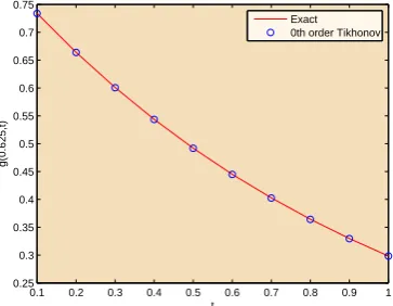
The exact solution of this problem is u(x, y, t) = e−t(sin(x) + cos(y)) and g(y, t) = e−tcos(y). The results obtained for u(0, y, t) with tf = 1, ∆t = 0.1,0.01, y = 0.625

andM1 =M2 = 4 with noisy data (noisy data=input data+(0.01)rand(1)) are presented

in Tables 1, 2 and Figures 1-6.

t Exact 0th order Tikhonov 1st order Tikhonov 2nd order Tikhonov

0.1 0.733790 0.733754 0.733675 0.733675

0.2 0.663960 0.663824 0.663665 0.663835

0.3 0.600776 0.600489 0.600501 0.600456

0.4 0.543605 0.543430 0.543430 0.543314

0.5 0.491874 0.491800 0.491649 0.491684

0.6 0.445066 0.444882 0.444944 0.444996

0.7 0.402712 0.402423 0.402514 0.402475

0.8 0.364389 0.364217 0.364052 0.364142

0.9 0.329713 0.329665 0.329381 0.329643

1 0.298337 0.298281 0.298181 0.298283

S 1.369e−004 1.933e−004 1.599e−004

Table 1. The comparison between exact solution and Tikhonov’s solutions for g(0.625, t)

(16)

0.01 0.802894 0.802883 0.802794 0.802749

0.02 0.794905 0.794792 0.794795 0.794750

0.1 0.733790 0.733543 0.733569 0.733683

0.11 0.726488 0.726247 0.726349 0.726286

0.5 0.491874 0.491679 0.491646 0.491723

0.51 0.486980 0.486713 0.486739 0.486785

0.8 0.364389 0.364160 0.364127 0.364190

0.81 0.360763 0.360536 0.360607 0.360566

0.9 0.329713 0.329528 0.329526 0.329567

0.91 0.326432 0.326244 0.326178 0.326194

1 0.298337 0.298255 0.298105 0.298215

S 1.600e−004 1.615e−004 1.471e−004

with the noisy data when ∆t= 0.01.

0.1 0.2 0.3 0.4 0.5 0.6 0.7 0.8 0.9 1

0.25 0.3 0.35 0.4 0.45 0.5 0.55 0.6 0.65 0.7 0.75

t

g(0.625,t)

Exact 0th order Tikhonov

Figure 1. The comparison between the exact solution and 0th order Tikhonov solution

forg(0.625, t) with noisy data when ∆t= 0.1.

0.1 0.2 0.3 0.4 0.5 0.6 0.7 0.8 0.9 1

0.25 0.3 0.35 0.4 0.45 0.5 0.55 0.6 0.65 0.7 0.75

t

g(0.625,t)

Exact 1st order Tikhonov

Figure 2. The comparison between the exact solution and 1st order Tikhonov solution

(17)

0.1 0.2 0.3 0.4 0.5 0.6 0.7 0.8 0.9 1 0.25

0.3 0.35 0.4 0.45 0.5 0.55 0.6 0.65 0.7 0.75

t

g(0.625,t)

Exact 2nd order Tikhonov

Figure 3. The comparison between the exact solution and 2nd order Tikhonov solution

0 0.2 0.4 0.6 0.8 1

0 1 2

x 10−4

t

g(0.625,t)

Exact

−g(0.625,t)

0th order Tikhonov

Line 0

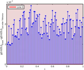
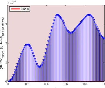
Figure 4. Diﬀerence between the the exact solution and 0th order Tikhonov solution for

g(0.625, t) of problem (1.5) with noisy data when ∆t= 0.01.

0 0.2 0.4 0.6 0.8 1

0 1 2

x 10−4

t

g(0.625,t)

Exact

−g(0.625,t)

1st order Tikhonov

Line 0

Figure 5. Diﬀerence between the the exact solution and 1st order Tikhonov solution for

(18)

0 0.2 0.4 0.6 0.8 1 0

1 2

x 10−4

t

g(0.625,t)

Exact

−g(0.625,t)

2nd order Tikhonov

Line 0

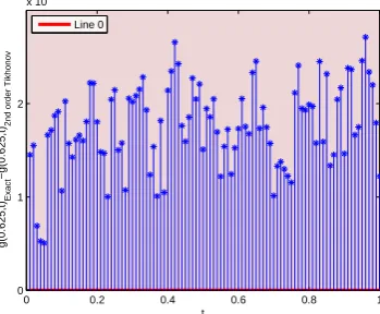
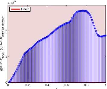
Figure 6. Diﬀerence between the the exact solution and 2nd order Tikhonov solution for

Example 2. In this example we solve the problem (2.2)with given data,

u(x, y,0) = sinh(x) + cosh(y), 0≤x≤1,0≤y ≤1,

ut(x, y,0) = sinh(x) + cosh(y), 0≤x≤1,0≤y ≤1,

u(1, y, t) =et(sinh 1 + cosh(y)), 0≤y≤1,0≤t≤tf,

u(x,0, t) =et(sinh(x) + 1), 0≤x≤1,0≤t≤tf,

u(x,1, t) =et(sinh(x) + cosh 1), 0≤x≤1,0≤t≤tf,

u(0.1, y, t) =et(sinh 0.1 + cosh(y)), 0≤y≤1,0≤t≤tf.

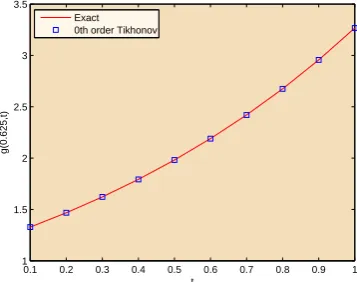
The exact solution of this problem is u(x, y, t) = et(sinh(x) + cosh(y)) and g(y, t) =

etcosh(y). The results obtained for u(0, y, t) with tf = 1, ∆t = 0.1,0.01, y = 0.625

andM1 =M2 = 4 with noisy data (noisy data=input data+(0.01)rand(1)) are presented

in Tables 3, 4 and Figures 7-12.

0.1 1.328143 1.328061 1.328121 1.328117

0.2 1.467825 1.467701 1.467750 1.467738

0.3 1.622198 1.621092 1.622116 1.622079

0.4 1.792806 1.792647 1.792716 1.792670

0.5 1.981357 1.981102 1.981207 1.981103

0.6 2.189738 2.189501 2.189565 2.189370

0.7 2.420035 2.419809 2.419820 2.419651

0.8 2.674552 2.674289 2.674297 2.674155

0.9 2.955837 2.955653 2.955595 2.955440

1 3.266705 3.266575 3.266431 3.266361

S 1.617e−004 1.500e−004 2.350e−004

(19)

0.01 1.213832 1.213829 1.213831 1.213830

0.02 1.226031 1.226024 1.226028 1.226026

0.1 1.328143 1.328038 1.328051 1.328086

0.11 1.341491 1.341375 1.341386 1.341426

0.5 1.981357 1.981082 1.981011 1.981148

0.51 2.001270 2.000993 2.000920 2.001058

0.8 2.674552 2.674240 2.674216 2.674274

0.81 2.701432 2.701130 2.701090 2.701157

0.9 2.955837 2.955637 2.955527 2.955637

0.91 2.985544 2.985344 2.985246 2.985352

1 3.266705 3.266459 3.266480 3.266522

S 1.763e−004 1.998e−004 1.551e−004

with noisy data when ∆t= 0.01.

0.1 0.2 0.3 0.4 0.5 0.6 0.7 0.8 0.9 1

1 1.5 2 2.5 3 3.5

t

g(0.625,t)

Exact 0th order Tikhonov

Figure 7. The comparison between the exact solution and 0th order Tikhonov solution

0.1 0.2 0.3 0.4 0.5 0.6 0.7 0.8 0.9 1

1 1.5 2 2.5 3 3.5

t

g(0.625,t)

Exact 1st order Tikhonov

Figure 8. The comparison between the exact solution and 1st order Tikhonov solution

(20)

0.1 0.2 0.3 0.4 0.5 0.6 0.7 0.8 0.9 1 1

1.5 2 2.5 3 3.5

t

g(0.625,t)

Exact 2nd order Tikhonov

Figure 9. The comparison between the exact solution and 2nd order Tikhonov solution

0 0.2 0.4 0.6 0.8 1

0 0.5 1 1.5 2 2.5 3 3.5x 10

−4

t

g(0.625,t)

Exact

−g(0.625,t)

0th order Tikhonov

Line 0

Figure 10. Diﬀerence between the the exact solution and 0th order Tikhonov solution for

0 0.2 0.4 0.6 0.8 1

0 1 2 3

x 10−4

t

g(0.625,t)

Exact

−g(0.625,t)

1st order Tikhonov

Line 0

Figure 11. Diﬀerence between the the exact solution and 1st order Tikhonov solution for

(21)

0 0.2 0.4 0.6 0.8 1 0

1 2

x 10−4

t

g(0.625,t)

Exact

−g(0.625,t)

2nd order Tikhonov

Line 0

Figure 12. Diﬀerence between the the exact solution and 2nd order Tikhonov solution

forg(0.625, t) of problem (2.2) with noisy data when ∆t= 0.01.

4. Conclusion

A numerical method, is proposed to estimate unknown boundary condition for these kinds of inverse problems in two-dimensional parabolic and hyperbolic equations and the following results are obtained.

1. The present study successfully applies the numerical method to inverse problems for two-dimensional parabolic and hyperbolic equations.

2. Numerical results show that a good estimation can be obtained within a couple of minutes CPU time at pentium IV-2.53 GHz PC.

3. The present method has been found stable with respect to small perturbation in the input data.

4. Numerical results show that, unknown function, evolutions estimated by the 0th order, 1st order and 2nd order Tikhonov regularization methods give very similar results.

References

[1] Abtahi, M., Pourgholi, R. and Shidfar, A., (2011), Existence and uniqueness of solution for a two dimensional nonlinear inverse diﬀusion problem, Nonlinear Analysis: Theory, Methods & Applications, 74, 2462-2467.

[2] Alifanov, O. M., (1994), Inverse Heat Transfer Problems, Springer, NewYork.

[3] Beck, J. V., Blackwell, B. and Clair, C. R. St., (1985), Inverse Heat Conduction: IllPosed Problems, Wiley-Interscience, NewYork.

[4] Beck, J. V., Blackwell, B. and Haji-sheikh, A., (1996), Comparison of some inverse heat conduction methods using experimental data, Internat. J. Heat Mass Transfer, 3, 3649-3657.

[5] Beck, J. V. and Murio, D. C., (1986), Combined function speciﬁcation-regularization procedure for solution of inverse heat condition problem, AIAA J., 24, 180-185.

[6] Cabeza, J. M. G, Garcia, J. A. M and Rodriguez, A. C., (2005), A Sequential Algorithm of Inverse Heat Conduction Problems Using Singular Value Decomposition, International Journal of Thermal Sciences, 44, 235-244.

[7] Chen, C. F. and Hsiao, C. H., (1997), Haar wavelet method for solving lumped and distributed-parameter systems, IEE Proc.: part D, 144 (1), 87-94.

[8] Chen, H. T. and Lin, J. Y., (1993, 1994), Analysis of two-dimensional hyperbolic heat conduction problems, lnt, J. Heat Mass Transfer, 37 (1), 153164.

[9] Ching-yu, Y., (2009), Direct and inverse solutions of the two-dimensional hyperbolic heat conduction problems, Appl. Math. Model., 33, 2907-2918.

[10] Elden, L., (1984), A Note on the Computation of the Generalized Cross-validation Function for Ill-conditioned Least Squares Problems, BIT, 24, 467-472.

(22)

[12] Haar, A., (1910), Zur theorie der orthogonalen Funktionsysteme, Math. Annal., 69, 331-371.

[13] Hansen, P. C., (1992), Analysis of discrete ill-posed problems by means of the L-curve, SIAM Rev, 34, 561-580.

[14] Hariharan, G., Kannan, K. and Sharma, K. R., (2009), Haar wavelet method for solving Fisher’s equation, Applied Mathematics and Computation, 211, 284-292.

[15] Hsiao, C. H. and Wang, W. J., (2001), Haar wavelet approach to nonlinear stiﬀ systems, Math. Comput. Simul., 57, 347-353.

[16] Huang, C.-H. and Tsai, Y.-L., (2005), A transient 3-D inverse problem in imaging the time- depen-dentlocal heat transfer coeﬃcients for plate ﬁn, Applied Therma Engineering, 25, 2478-2495. [17] Huang, C.-H., Yeha, C.-Y. and Orlande, H. R. B., (2003), A nonlinear inverse problem in

simul-taneously estimating the heat and mass production rates for a chemically reacting ﬂuid, Chemical Engineering Science, 58 (16), 3741-3752.

[18] Kalpana, R. and Raja Balachandar, S., (2007), Haar wavelet method for the analysis of transistor circuits, Int. J.Electron. Commun. (AEU), 61, 589-594.

[19] Lawson, C. L. and Hanson, R. J., (1995), Solving Least Squares Problems, Philadelphia, PA: SIAM. [20] Martin, L., Elliott, L., Heggs, P. J., Ingham, D. B., Lesnic, D. and Wen, X., (2006), Dual

Reci-procity Boundary Element Method Solution of the Cauchy Problem for Helmholtz-type Equations with Variable Coeﬃcients, Journal of sound and vibration, 297, 89-105.

[21] Molhem, H. and Pourgholi, R., (2008), A numerical algorithm for solving a one-dimensional inverse heat conduction problem, Journal of Mathematics and Statistics, 4 (1), 60-63.

[22] Murio, D. A., (1993), The Molliﬁcation Method and the Numerical Solution of Ill-Posed Problems, Wiley-Interscience, New York.

[23] Murio, D. C. and Paloschi, J. R., (1988), Combined molliﬁcation-future temperature procedure for solution of inverse heat conduction problem, J. Comput. Appl. Math., 23, 235-244.

[24] Pourgholi, R., Azizi, N., Gasimov, Y. S., Aliev, F. and Khalaﬁ, H. K., (2009), Removal of Numerical Instability in the Solution of an Inverse Heat Conduction Problem, Communications in Nonlinear Science and Numerical Simulation, 14 (6), 2664-2669.

[25] Pourgholi, R. and Rostamian, M., (2010), A numerical technique for solving IHCPs using Tikhonov regularization method, Applied Mathematical Modelling, 34 (8), 2102-2110.

[26] Pourgholi, R., Rostamian, M. and Emamjome, M., (2010), A numerical method for solving a nonlinear inverse parabolic problem, Inverse Problems in Science and Engineering, 18 (8), 1151-1164.

[27] Sun, K. K., Jung, B. S. and Lee, W. l., (2007), An inverse estimation of surface temperature using the maximum entropy method, International Communication of Heat and Mass Transfer, 34, 37-44. [28] Su, J. and Silva Neto, A. J., (2001), Two-dimensional inverse heat conduction problems of source

strength estimation in cylindrical rods, Applied Mathematical Modelling, 25, 861-872.

[29] Tadi, M., (1997), Inverse Heat Conduction Based on Boundary Measurement, Inverse Problems, 13, 1585-1605.

[30] Tikhonov, A. N. and Arsenin, V. Y., (1977), On the solution of ill-posed problems, New York, Wiley. [31] Tikhonov, A. N. and Arsenin, V. Y., (1977), Solution of Ill-Posed Problems, V. H. Winston and Sons,

Washington, DC.