THE METHOD OF LINES FOR THE NUMERICAL SOLUTION OF A MATHEMATICAL MODEL IN THE INITIATION OF ANGIOGENESIS
S. PAMUK1, I. ATAC2 §
Abstract. In this paper we present the method of lines to obtain the numerical solution
of a mathematical model for the roles of endothelial, pericyte and macrophage cells in the initiation of tumor angiogenesis. This method is an approach to the numerical solution of partial differential equations that involve a time variable t and a space variable x. We provide computer programs written in Matlab. Also, the stability analysis of the solutions is given, and the figures for endothelial, pericyte and macrophage cell movements in the capillary are presented for large times.
Keywords: Method of lines, stability, angiogenesis, capillary AMS Subject Classification: 65M20, 34D20
1. Introduction
Angiogenesis is the main feature of the formation of new blood vessels. The abluminal surface of the capillaries is covered by a collageneous network intermingled with laminin which is called the basal lamina (BL). The BL is mainly formed by the Endothelial Cells (EC). In the neighborhood of BL, there are other cell types such as Pericyte Cells (PC) and Macrophage Cells (MC) [4].
In this paper we consider the following initial boundary-value problem originally pre-sented in [4]:
∂η ∂t =D1
∂ ∂x
(
η ∂ ∂x
(
ln η
τ1 ))
,0< x <1,0< t≤T, (1)
∂σ ∂t =D2
∂ ∂x
(
σ ∂ ∂x
(
ln σ
τ2 ))
,0< x <1, 0< t≤T, (2)
∂m ∂t =D3
∂ ∂x
(
m ∂
∂x
(
lnm
τ3 ))
,0< x <1,0< t≤T, (3)
whereη(x, t), σ(x, t) andm(x, t) are the concentrations of EC, PC and MC, respectively, and τ1, τ2 and τ3 are the transition probability functions of them. Also, D1, D2, D3 are
EC, PC and MC diffusion constants. We impose the initial conditions,
η(x,0) = 1, σ(x,0) = 1, m(x,0) = 1, 0< x <1, (4) and the boundary conditions,
1 Department of Mathematics, University of Kocaeli, Umuttepe Campus, 41380, Kocaeli - TURKEY, e-mail: [email protected]
2 Department of Mathematics, University of Kocaeli, Umuttepe Campus, 41380, Kocaeli - TURKEY, e-mail: [email protected]
§ Manuscript received April 04, 2013.
TWMS Journal of Applied and Engineering Mathematics Vol.3, No.1; c⃝I¸sık University, Department of Mathematics, 2013; all rights reserved.
D1η ∂ ∂x ( ln η τ1 ) x=0
=D2σ
∂ ∂x ( ln σ τ2 ) x=0
=D3m
∂ ∂x ( lnm τ3 ) x=0
= 0, (5)
D1η
∂ ∂x ( ln η τ1 ) x=1
=D2σ
∂ ∂x ( ln σ τ2 ) x=1
=D3m
∂ ∂x ( lnm τ3 ) x=1
= 0. (6)
As in [6,7], for numerical purposes we take the transition probability functions τ1, τ2
andτ3 as follows:
τ1=f(x) = (
α1+Axn(1−x)n
α2+Axn(1−x)n
)γ1(β
1+ 1−Bxn(1−x)n
β2+ 1−Bxn(1−x)n )γ2
, (7)
τ2=g(x) = (
α3+ 1−Bxn(1−x)n
α4+ 1−Bxn(1−x)n )γ3
, (8)
τ3=r(x) = (
β3+Axn(1−x)n
β4+Axn(1−x)n )γ4
. (9)
Here, n,A,B,αi,βi and γi (i= 1 : 4) are some positive constants which we take here
to be the same as in [4]. The Authors of Ref.[4] have chosen the transition probability functionsf(x), g(x) andr(x) more complicated for biological reasons. But for simplicity, we take them as a function ofx only.
2. Method
The method of lines (MOL) is a general way of viewing a partial differential equation (PDE) as a system of ordinary differential equations (ODE) [1-3,5,6,9-11]. The partial derivatives with respect to the space variables are discretized to obtain a system of ODEs in the time variable and then a suitable initial-value problem solver is used to solve this ODE system. This method has the broad applicability to physical and chemical systems modeled by PDEs [9]. Also, this method provides very accurate numerical solution for linear or nonlinear PDE’ s in comparison with other existing methods [6]. As the number of lines increases, the accuracy of the MOL representation of the original system increases [5]. We now apply this method to our problem given by Eqs.(1)-(6).
We proceed uniform grid,
W ={(xi, tj) :xi = (i−1)h, tj = (j−1)k, i= 1 :M, j = 1 :N, h= 1/(M−1), k=
1/(N−1)}and obtain a difference scheme for the problem in Eqs.(1)-(6). Eqs.(1)-(3) can be written as follows:
ηt=D1(ηxx−(ηF)x), (10)
σt=D2(σxx−(σG)x), (11)
mt=D1(mxx−(mH)x), (12)
where F = f
′(x)
f(x),G=
g′(x)
g(x) and H =
r′(x)
r(x).
We suppose the solutions of Eqs.(10)-(12) η(x, t), σ(x, t) and m(x, t) can be approxi-mated byηi, σi andmi,respectively, and use the standart difference equations for the first
and the second derivatives of these variables. Therefore, by discretizing the right handside of Eqs.(10)-(12) we obtain the following system of ODE’s:
dηi
dt =D1
(
ηi+1−2ηi+ηi−1
h2 −
ηi+1Fi+1−ηi−1Fi−1
2h
)
dσi
dt =D2
(
σi+1−2σi+σi−1
h2 −
σi+1Gi+1−σi−1Gi−1
2h
)
, (14)
dmi
dt =D3
(
mi+1−2mi+mi−1
h2 −
mi+1Hi+1−mi−1Hi−1
2h
)
. (15)
The initial conditions in Eq.(4) and boundary conditions in Eqs.(5)-(6) now become:
ηi= 1, σi = 1,mi = 1, 1< i < M,t= 0, (16)
D1 (
∂η1
∂x −η1F1
)
= 0, fort >0, (17)
D1 (
∂ηM
∂x −ηMFM
)
= 0, for t >0, (18)
D2 (
∂σ1
∂x −σ1G1
)
= 0, fort >0, (19)
D2 (
∂σM
∂x −σMGM
)
= 0, fort >0, (20)
D3 (
∂m1
∂x −m1H1
)
= 0, for t >0, (21)
D3 (
∂mM
∂x −mMHM
)
= 0, fort >0. (22)
Using the central difference for the boundary conditions in Eqs.(17)-(22) and taking into account Eqs.(13)-(15), we obtain the following system of ODE’s:
dη1
dt =D1
(
2η2−2(1 +hF1)η1
h2 −
η2F2−(η2−2hη1F1)F0
2h
)
, (23)
dηi
dt =D1
(
ηi+1−2ηi+ηi−1
h2 −
ηi+1Fi+1−ηi−1Fi−1
2h
)
, 1< i < M, (24)
dηM
dt =D1
(
2ηM−1−2(1−hFM)ηM
h2 −
(ηM−1+ 2hηMFM)FM+1−ηM−1FM−1
2h
)
, (25)
dσ1
dt =D2
(
2σ2−2(1 +hG1)σ1
h2 −
σ2G2−(σ2−2hσ1G1)G0
2h
)
, (26)
dσi
dt =D2
(
σi+1−2σi+σi−1
h2 −
σi+1Gi+1−σi−1Gi−1
2h
)
, 1< i < M, (27)
dσM
dt =D2
(
2σM−1−2(1−hGM)σM
h2 −
(σM−1+ 2hσMGM)GM+1−σM−1GM−1
2h
)
,(28)
dm1
dt =D3
(
2m2−2(1 +hH1)m1
h2 −
m2H2−(m2−2hm1H1)H0
2h
)
, (29)
dmi
dt =D3
(
mi+1−2mi+mi−1
h2 −
mi+1Hi+1−mi−1Hi−1
2h
)
, 1< i < M, (30)
dmM
dt =D3
(
2mM−1−2(1−hHM)mM
h2 −
(mM−1+ 2hmMHM)HM+1−mM−1HM−1
2h
)
.
3. Stability of the solutions
We let
x= [η1 · · · ηi · · · ηM σ1 · · · σi · · · σM m1 · · · mi · · · mM]T (32)
and f(x)= D1 (
2η2−2(1+hF1)η1
h2 −
η2F2−(η2−2hη1F1)F0
2h ) .. . D1 (
ηi+1−2ηi+ηi−1
h2 −
ηi+1Fi+1−ηi−1Fi−1
2h ) .. . D1 (
2ηM−1−2(1−hFM)ηM
h2 −
(ηM−1+2hηMFM)FM+1−ηM−1FM−1
2h
)
D2 (
2σ2−2(1+hG1)σ1
h2 −
σ2G2−(σ2−2hσ1G1)G0
2h ) .. . D2 (
σi+1−2σi+σi−1
h2 −
σi+1Gi+1−σi−1Gi−1
2h ) .. . D2 (
2σM−1−2(1−hGM)σM
h2 −
(σM−1+2hσMGM)GM+1−σM−1GM−1
2h
)
D3 (
2m2−2(1+hH1)m1
h2 −
m2H2−(m2−2hm1H1)H0
2h ) .. . D3 (
mi+1−2mi+mi−1
h2 −
mi+1Hi+1−mi−1Hi−1
2h ) .. . D3 (
2mM−1−2(1−hHM)mM
h2 −
(mM−1+2hmMHM)HM+1−mM−1HM−1
2h ) , (33)
where 2≤i≤M−1. Then, by Eqs.(23)-(31) one has the following autonomous system of ordinary differential equations:
˙
x=f(x), t≥0. (34)
We now let
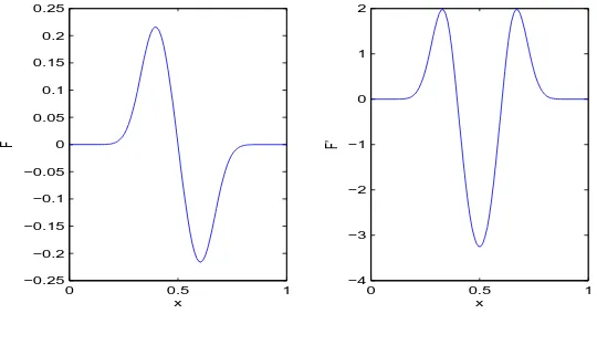
η(x, t) = 1 +η∗(x, t), σ(x, t) = 1 +σ∗(x, t), m(x, t) = 1 +m∗(x, t), (35) and assume that F′(x) ≈0, G′(x) ≈0, H′(x) ≈0 for small x. These assumptions are reasonable (see Figures (1)-(3)). Therefore, Eqs.(10)-(15) and Eqs.(17)-(31) stay the same in the variables with the asterisks except the initial conditions in Eq.(16) now become
η∗i = 0,σ∗i = 0,m∗i = 0, 1< i < M,t= 0. (36)
For simplicity we drop all of the asterisks. Therefore, we now solve Eqs.(23)-(31) with the initial conditions in Eq.(36).
It is now clear to see that the only steady-state solution to Eqs.(23)-(31) is the vector
c = (0· · ·0 0· · ·0 0· · ·0)T of length 3M. Let A, B and C be the matrices of first order partial derivatives off(x) with respect to the variables ηi,σi and mi (1≤i≤M),
A=
−D1(2(1+hFh2 1)+F1F0) D1(h22−
F2
2h+ F0
2h) 0 · · · 0
D1(h12 +
F1
2h) −
2D1
h2 D1(h12 −
F3
2h)
. . .
0 . .. . .. . .. 0
. .
. D1(h12+
FM−2
2h ) − 2D1
h2 D1(h12−
FM
2h)
0 · · · 0 0 D1(2hFhM2−2−FMFM+1)
B=
−D2(2(1+hGh2 1)+G1G0) D2(h22 −
G2
2h+ G0
2h) 0 · · · 0
D2(h12+
G1
2h) −
2D2
h2 D2(h12−
G3
2h)
. . .
0 . .. . .. . .. 0
. .
. D2(h12 +
GM−2
2h ) − 2D2
h2 D2(h12−
GM 2h)
0 · · · 0 0 D2(2hGhM2−2−GMGM+1)
C=
−D3(2(1+hHh2 1)+H1H0) D3(h22 −
H2
2h + H0
2h) 0 · · · 0
D3(h12 +
H1
2h) −
2D3
h2 D3(h12−
H3
2h)
. . .
0 . .. . .. . .. 0
. .
. D3(h12+
HM−2
2h ) − 2D3
h2 D3(h12−
HM
2h)
0 · · · 0 0 D3(2hHhM2−2−HMHM+1)
We let S =
A B O
O C
where O is the zero matrix. It is well known that the determinant of the matrixS is the product of the determinants of the matricesA, B and C. Therefore, the eigenvalues of S consists of the set of eigenvalues of A, B and C. We know that every solution of the system of equations given by Eqs.(23)-(31) is stable if all the eigenvalues of S have negative real part and unstable if at least one eigenvalue ofS has positive real part [12].
In the following section we solve the system in Eqs.(23)-(31) with the initial conditions in Eq.(36) by using an ordinary differential equation solver which is built up in Matlab, and discuss the stability (or unstability) of the solutions of the system by determining the signs of the real parts of the eigenvalues of the matrixS for some values of M.
4. Numerical experiments
First, we solve the system in Eqs.(23)-(31) by the method of lines. For numerical purposes we take the following constants and parameters from [4,6,7]. D1 =D2 =D3 =
0.00025, α1 = 0.1, α2 = 2, α3 = 0.15, α4 = 1, β1 = 10, β2 = 0.1, β3 = 0.5, β4 = 1, γ1 =
1, γ2 = 1, γ3 = 1, γ4 = 1, n= 16, A= 28×107, B= 0.22×10⁹.We first code the input data
concentration (see Section 5.1 for Matlab codes). These concentrations are shown in Figs. 4-7, respectively. Furthermore, the importance of these concentrations in the initiation of angiogenesis is explained in Conclusions.
Second, we test the signs of the real parts of the eigenvalues of the matrix S for the system in Eqs.(23)-(31) (see Section 5.2 for the construction of the matrixS in Matlab). We do this by assuming F′(x) ≈ 0, G′(x) ≈ 0, H′(x) ≈ 0 for small x, and taking
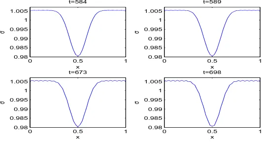
M = 21,23,25,27,29,31,41, and 45, respectively. When M = 21,23,25,27,29,31 we observe that the real parts of the eigenvalues of S are negative (see Table 1), and thus all of the solutions of our system are stable for large time levels [12]. Figs. 4-6 are some snapshots taken at t= 10,110,210,310,410,510,610 and t= 710. This is a strong evidence that all of the solutions of our system are stable for all time levels. But, when
M = 41 andM = 45 we see that the real parts of two of the eigenvalues ofS are positive (see Table 1), which means that every solution of our system is unstable. As it is clear from the Fig.7 that the stability changes to unstability around t = 589. As users may remember the ODE solver ”ode45” which is built up in Matlab chooses its time step ”k” automatically. One of the reason we get unstability forM = 45 as time increases may be the violation of the CFL condition
Dik
h2 ≤
1
2, (i= 1,2,3),
where Di are the diffusion constants and h = 1/(M−1). As M increases one has to
takekvery small to meet the CFL condition since Di are fixed constants. Therefore, the
CFL condition is a severe restriction on time step.
The other reason for the unstability for M = 45 case could be the rounding errors in our computations. Although rounding errors can excite an unstability, more often it is discretisation errors that do so.
Fig.7 would have looked the same even if the computations had been carried out by using stiff ODE solvers built up in Matlab such as ode15s, ode23s.
Of course, a fully implicit or the Crank-Nicolson method can be used to address the unstability for most of the problems in PDEs. Although there is no restriction on time step for both methods, they require more work at each time step. Especially the Crank-Nicolson method is unconditionally stable.
0 0.5 1
−0.25 −0.2 −0.15 −0.1 −0.05 0 0.05 0.1 0.15 0.2 0.25
x
F
0 0.5 1
−4 −3 −2 −1 0 1 2
x
F’
0 0.5 1 −0.2
−0.15 −0.1 −0.05 0 0.05 0.1 0.15 0.2
x
G
0 0.5 1
−2 −1 0 1 2 3 4
x
G’
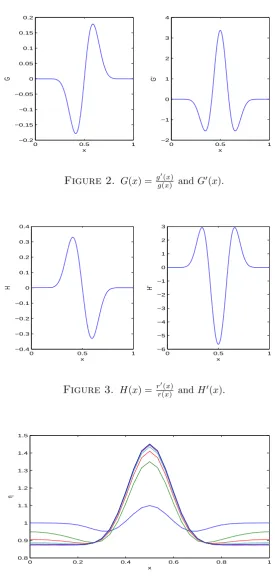
Figure 2. G(x) =gg′((xx)) andG′(x).
0 0.5 1
−0.4 −0.3 −0.2 −0.1 0 0.1 0.2 0.3 0.4
x
H
0 0.5 1
−6 −5 −4 −3 −2 −1 0 1 2 3
x
H’
Figure 3. H(x) = rr′((xx)) andH′(x).
0 0.2 0.4 0.6 0.8 1
0.8 0.9 1 1.1 1.2 1.3 1.4 1.5
x
η
0 0.2 0.4 0.6 0.8 1 0.98
0.985 0.99 0.995 1 1.005
x
σ
Figure 5. PC Concentrationσ(x, t) withM = 31.
0 0.2 0.4 0.6 0.8 1
0.98 0.99 1 1.01 1.02 1.03 1.04 1.05
x
m
Figure 6. MC Concentrationm(x, t) withM = 31.
0 0.5 1
0.98 0.985 0.99 0.995 1 1.005
x
σ
t=584
0 0.5 1
0.98 0.985 0.99 0.995 1 1.005
x
σ
t=589
0 0.5 1
0.98 0.985 0.99 0.995 1 1.005
x
σ
t=673
0 0.5 1
0.98 0.985 0.99 0.995 1 1.005
x
σ
t=698
M=21 M=23 M=25 M=27 M=29 M=31 M=41 M=45 -0.1156 -1.4472 0.0000 -0.0388 -1.3657 -0.0025 -0.4500 -1.3196 -0.0097 -1.2702 -0.0222 -1.1632 -0.0391 -0.8628 -0.0610 -0.9251 -0.0875 -1.1061 -0.1184 -0.7372 -0.1537 -0.9868 -0.1931 -0.6749 -0.2364 0.0000 -0.2835 -0.6132 -0.3341 -0.4939 -0.3879 -0.4368 -0.4447 -0.0025 -0.5041 -0.3298 -0.5659 -0.1179 -0.6297 -0.0391 -0.6953 -0.0222 -0.7622 -0.1528 -0.8302 -0.2804 -0.8989 -0.2343 -0.9680 -0.0872 -1.0371 -1.0472 -1.1058 -1.2180 -1.1738 -0.5528 -1.2407 -0.0609 -1.3063 -0.3820 -1.3701 -1.4083 -1.4319 -0.0097 -1.4913 -0.1917 -1.5481 -0.8000 -1.6019 -1.9360 -1.9335 -1.9263 -1.9138 -1.8969 -1.8750 -1.8485 -1.8176 -1.7823 -1.7429 -1.6996 -1.6525
Table 1: Real Parts of the Eigenvalues of the MatrixS for some Values ofM
5. Conclusions
unrealistic assumptions. As the number of lines increases, the accuracy of the MOL representation increases. This method is also applicable to non-linear systems of PDEs. In Figs. 4-6, we have plotted the EC, PC and MC concentrations for large times. Notice that pericyte aggregation in the opening in the capillary wall is low where the EC and MC concentrations are high and conversely. In particular, the maximum of PC density is higher closer to the wall of the forming capillary than is the maximum of EC density [4]. These are consistent with the observations of [8] that the PC closely regulate the development of the forming channel.
We have also showed that when M = 21,23,25,27,29,31 all of the solutions of our system obtained from the discretisation of the space variablex are stable. This a strong evidence that all of the solutions are stable for all time levels as it is clear from the Figs. 4-6. To show the stability of the solutions, we have obtained (in Table 1) the negativity of the real parts of the eigenvalues of the matrix (namelyS) consisting of the first order partial derivatives of the discretised vectoral function with respect to the unknown variables, evaluated at a constant steady state solution.
When we increase M we have faced that the real parts of two of the eigenvalues of the matrix S are positive, which means that every solution of our system is unstable. For example, whenM = 45 the stability changes to unstability around t= 589 as it is clear from the Fig. 7, which may be caused by the violation of the CFL condition.
We have also presented our Matlab codes in the Appendix A and B below, which may enlighten young researchers to learn one of the numerical methods to solve PDEs or systems of PDEs.
6. Appendix A
Matlab codes for the method of lines
%%%%%%%%%%%%%%%%%%%%%%%%%%%%%%%%%%%% function z=fparabolic(t,w)
global h M
alpha1=0.1; alpha2=2; alpha3=0.15; alpha4=1; beta1=10; beta2=0.1; beta3=0.5; beta4=1; gama1=1;
gama2=1; gama3=1; gama4=1; D1=0.00025; D2=0.00025; D3=0.00025; n=16; A=28*10ˆ7; B=0.22*10ˆ9;
eta=w(1:M); sigma=w(M+1:2*M); m=w(2*M+1:3*M); h=1./(M-1);
%%%%%%%%%%%%%% F,G,H functions%%%%%%%%%%%%%%% for i=1:M
x(i)=(i-1)*h; % the vector x end
F0=gama1*(alpha2-alpha1)*A*n*(-h-hˆ2)ˆ(n-1)*(1+2*h)/... ((alpha1+A*(-h-hˆ2)ˆn)*(alpha2+A*(-h-hˆ2)ˆn))+...
gama2*(beta1-beta2)*B*n*(-h-hˆ2)ˆ(n-1)*(1+2*h)/...
((beta1+1-B*(-h-hˆ2)ˆn)*(beta2+1-B*(-h-hˆ2)ˆn)); % F(x) at x=0 G0=gama3*(alpha3-alpha4)*B*n*(-h-hˆ2)ˆ(n-1)*(1+2*h)/...
((alpha3+1-B*(-h-hˆ2)ˆn)*(alpha4+1-B*(-h-hˆ2)ˆn)); % G(x) at x=0 H0=gama4*(beta4-beta3)*A*n*(-h-hˆ2)ˆ(n-1)*(1+2*h)/...
((beta3+A*(-h-hˆ2)ˆn)*(beta4+A*(-h-hˆ2)ˆn)); % H(x) at x=0 for i=1:M
gama2*(beta1-beta2)*B*n*(x(i)-x(i)ˆ2)ˆ(n-1)*(1-2*x(i))/...
((beta1+1-B*(x(i)-x(i)ˆ2)ˆn)*(beta2+1-B*(x(i)-x(i)ˆ2)ˆn)); % F(x) in the interval 0<x<1
G(i)=gama3*(alpha3-alpha4)*A*n*(x(i)-x(i)ˆ2)ˆ(n-1)*(1-2*x(i))/...
((alpha3+1-A*(x(i)-x(i)ˆ2)ˆn)*(alpha4+1-A*(x(i)-x(i)ˆ2)ˆn)); % G(x) in the inter-val 0<x<1
H(i)=gama4*(beta4-beta3)*B*n*(x(i)-x(i)ˆ2)ˆ(n-1)*(1-2*x(i))/...
((beta3+B*(x(i)-x(i)ˆ2)ˆn)*(beta4+B*(x(i)-x(i)ˆ2)ˆn)); % H(x) in the interval 0<x<1 end
F(M+1)=gama1*(alpha2-alpha1)*A*n*(M*h-(M*h)ˆ2)ˆ(n-1)*(1-2*M*h)/... ((alpha1+A*(M*h-(M*h)ˆ2)ˆn)*(alpha2+A*(M*h-(M*h)ˆ2)ˆn))+...
gama2*(beta1-beta2)*B*n*(M*h-(M*h)ˆ2)ˆ(n-1)*(1-2*M*h)/...
((beta1+1-B*(M*h-(M*h)ˆ2)ˆn)*(beta2+1-B*(M*h-(M*h)ˆ2)ˆn)); % F(x) at x=1 G(M+1)=gama3*(alpha3-alpha4)*A*n*(M*h-(M*h)ˆ2)ˆ(n-1)*(1-2*M*h)/...
((alpha3+1-A*(M*h-(M*h)ˆ2)ˆn)*(alpha4+1-A*(M*h-(M*h)ˆ2)ˆn)); % G(x) at x=1 H(M+1)=gama4*(beta4-beta3)*B*n*(M*h-(M*h)ˆ2)ˆ(n-1)*(1-2*M*h)/...
((beta3+B*(M*h-(M*h)ˆ2)ˆn)*(beta4+B*(M*h-(M*h)ˆ2)ˆn)); % H(x) at x=1 %%%%%%%%%%%%%%%%%%%%%%%%%%%%%%%%%%%%
z(1)=D1*((2*eta(2)-2*eta(1)-2*h*eta(1)*F(1))/hˆ2-...
(eta(2)*F(2)-(eta(2)-2*h*eta(1)*F(1))*F0)/(2*h)); % gives Eq. (23) z(M+1)=D2*((2*sigma(2)-2*sigma(1)-2*h*sigma(1)*G(1))/hˆ2-...
(sigma(2)*G(2)-(sigma(2)-2*h*sigma(1)*G(1))*G0)/(2*h)); % gives Eq. (26) z(2*M+1)=D3*((2*m(2)-2*m(1)-2*h*m(1)*H(1))/hˆ2-...
(m(2)*H(2)-(m(2)-2*h*m(1)*H(1))*H0)/(2*h)); % gives Eq. (29) for i=2:M-1;
z(i)=D1*((eta(i+1)-2*eta(i)+eta(i-1))/hˆ2-...
(eta(i+1)*F(i+1)-eta(i-1)*F(i-1))/(2*h)); % gives Eq. (24) z(M+i)=D2*((sigma(i+1)-2*sigma(i)+sigma(i-1))/hˆ2-...
(sigma(i+1)*G(i+1)-sigma(i-1)*G(i-1))/(2*h)); % gives Eq. (27) z(2*M+i)=D3*((m(i+1)-2*m(i)+m(i-1))/hˆ2-...
(m(i+1)*H(i+1)-m(i-1)*H(i-1))/(2*h)); % gives Eq. (30) end
z(M)=D1*((2*h*eta(M)*F(M)-2*eta(M)+2*eta(M-1))/hˆ2-...
((eta(M-1)+2*h*F(M)*eta(M))*F(M+1)-eta(M-1)*F(M-1))/(2*h)); % gives Eq. (25) z(2*M)=D2*((2*h*sigma(M)*G(M)-2*sigma(M)+2*sigma(M-1))/hˆ2-...
((sigma(M-1)+2*h*G(M)*sigma(M))*G(M+1)-sigma(M-1)*G(M-1))/(2*h)); % gives Eq. (28)
z(3*M)=D3*((2*h*m(M)*H(M)-2*m(M)+2*m(M-1))/hˆ2-...
((m(M-1)+2*h*H(M)*m(M))*H(M+1)-m(M-1)*H(M-1))/(2*h)); % gives Eq. (31) z=z’;
%%%%%%%%%%%%%%%%%%%%%%%%%%%%%%%%%%%% clc;clear all; global h M;
h=1/(M-1); %M=31,45 tf=751;% final time x=linspace(0,1,M); tspan=0:1:751; for i=1:M;
init=[eta0 sigma0 m0]; init=init’;
[t,y]=ode45(’fparabolic’,tspan,init); % solver that is built up in Matlab eta=y(:,1:M); sigma=y(:,M+1:2*M); m=y(:,2*M+1:3*M);
figure; % gives Fig.4
plot(x,eta(11:100:750,:)); xlabel(’x’); ylabel(’η’); figure; % gives Fig.5
plot(x,sigma(11:100:750,:));axis([0 1 0.98 1.007]); xlabel(’x’); ylabel(’σ’); figure; % gives Fig.6
plot(x,m(11:100:750,:)); xlabel(’x’); ylabel(’m’) figure; % gives Fig.7 tt=[585 590 674 699]; for i=1:4
subplot(2,2,i); plot(x,sigma(tt(i),:));axis([0 1 0.98 1.007]); xlabel(’x’); ylabel(’σ’); title([’t=’,num2str(tt(i)-1)]);
end
7. Appendix B
Matlab codes for the construction of the stability matrix S
%%%%%%%%%%%%%%%% S matrix%%%%%%%%%%%%%%%%%%%%
% All of the constants and functions in the following code are the same as in chapter 5.1.
S=zeros(3*M,3*M);
S(1,1)=-D1*(2*(1+h*F(1))/hˆ2+F0*F(1)); S(1,2)=D1*(2/hˆ2-F(2)/(2*h)+F0/(2*h)); for i=2:M-1
S(i,i-1)=D1*(1/hˆ2+F(i-1)/(2*h)); S(i,i)=-2*D1/hˆ2;
S(i,i+1)=D1*(1/hˆ2-F(i+1)/(2*h)); end
S(M,M-1)=D1*(2/hˆ2+F(M-1)/(2*h)-F(M+1)/(2*h)); S(M,M)=D1*((2*h*F(M)-2)/hˆ2-F(M)*F(M+1)); S(M+1,M+1)=-D2*(2*(1+h*G(1))/hˆ2+G0*G(1)); S(M+1,M+2)=D2*(2/hˆ2-G(2)/(2*h)+G0/(2*h)); for i=2:M-1
S(M+i,M+i-1)=D2*(1/hˆ2+G(i-1)/(2*h)); S(M+i,M+i)=-2*D2/hˆ2;
S(M+i,M+i-1)=D2*(1/hˆ2-G(i+1)/(2*h)); end
S(2*M,2*M-1)=D2*(2/hˆ2+G(M-1)/(2*h)-G(M+1)/(2*h)); S(2*M,2*M)=D2*((2*h*G(M)-2)/hˆ2-G(M)*G(M+1)); S(2*M+1,2*M+1)=-D3*(2*(1+h*H(1))/hˆ2+H0*H(1)); S(2*M+1,2*M+2)=D3*(2/hˆ2-H(2)/(2*h)+H0/(2*h)); for i=2:M-1
S(2*M+i,2*M+i-1)=D3*(1/hˆ2+H(i-1)/(2*h)); S(2*M+i,2*M+i)=-2*D3/hˆ2;
S(3*M,3*M-1)=D3*(2/hˆ2+H(M-1)/(2*h)-H(M+1)/(2*h)); S(3*M,3*M)=D3*((2*h*H(M)-2)/hˆ2-H(M)*H(M+1));
S; %The Matrix S
D=real(eig(S)); %The Real Parts of the Matrix S
References
[1] Ahmad, I. and Berzins, M., (2001), MOL solvers for hyperbolic PDEs with source terms, Math. Comput. Simulat., 56 (2), 115-125.
[2] Erdem, A. and Pamuk, S., (2007), The method of lines for the numerical solution of a mathematical model for capillary formation: The role of tumor angiogenic factor in the extra-cellular matrix, Appl. Math. Comput., 186, 891-897.
[3] Korn, G.A., (1999), Interactive solution of partial differential equations by the Method-of-lines, Math. Comput. Simulat., 49 (1-2), 129-138.
[4] Levine, H.A., Sleeman, B.D. and Nilsen-Hamilton, M., (2000), A mathematical model for the roles of pericytes and macrophages in the initiation of angiogenesis. I.The role of protease inhibitors in preventing angiogenesis, Math. Biosc., 168, 77-115.
[5] Mikhail, M.N., (1987), On the validity and stability of the method of lines for the solution of partial differential equations, Appl. Math. Comput., 22 (2-3), 89-98.
[6] Pamuk, S. and Erdem, A., (2007), The method of lines for the numerical solution of a mathematical model for capillary formation: The role of endothelial cells in the capillary, Appl. Math. Comput., 186, 831-835.
[7] Pamuk, S., (2003), Qualitative analysis of a mathematical model for capillary formation in tumor angiogenesis, Math. Models and Methods Apll. Sci., 13 (1), 19-33.
[8] Schor, A.M., Canfield, A.E., Sutton,A.B., Allen,T.D., Sloan,P., Schor, S.L., Steiner,R., Weisz, P.B. and Langer,R., (1992), The behavior of pericytes in vitro: relevance to angiogenesis and differentiation, Angiogenesis: Key Principles-Science-Technology-Medicine, Birkhauser, Basel.
[9] Shakeri, F. and Dehghan, M., (2008), The method of lines for solution of the one-dimensional wave equation subject to an integral conservation condition, Comput. and Math. with Appl., 56, 2175-2188. [10] Sharaf, A.A. and Bakodah, H.O., (2005), A good spatial discretisation in the method of lines, Appl.
Math. Comput., 171 (2), 1253-1263.
[11] Younes,A., Konz,M., Fahs, M., Zidane, A. and Huggenberger, P., (2011), Modelling variable den-sity flow problems in heterogeneous porous media using the method of lines and advanced spatial discretization methods, Math. Comput. Simulat., 81, 2346-2355.
[12] Teschl, G., (1991), Ordinary Differential Equations and Dynamical Systems, American Mathematical Society.
Serdal Pamukobtained his BSc in mathematics from Istanbul University