Sensor Placement in Water Distribution Networks based on Spectral Algorithms

Sensor Placement in Water Distribution

Networks based on Spectral Algorithms

Armando Di Nardo

, Carlo Giudicianni

, Roberto Greco

, Manuel

Herrera

, Giovanni Francesco Santonastaso

and Antonio Scala

Dipartimento di Ingegneria, Università degli Studi della Campania ‘L. Vanvitelli’, via Roma 29, Aversa 81031, Italia

2

Istituto dei Sistemi Complessi (Consiglio Nazionale delle Ricerche), via dei Taurini 19, Roma 00185, Italia

2

EDEn - Dept. of Architecture & Civil Engineering, University of Bath, Claverton Down, Bath BA2 7AZ, United Kingdom

[email protected], [email protected], [email protected], [email protected],

[email protected], [email protected]

Abstract

Installing an efficient monitoring and control sensor system provides the possibility to carry out main tasks on Water Distribution Networks (WDNs) management and protection. Given the WDNs complexity, efficient numerical techniques are needed to support optimal monitoring system design. Generally, it is appropriate to locate sensors at highly connected places in the WDN with water flow reaching several parts of the network. This paper introduces a general method to support water utilities on the decision making process for an efficient water system monitoring. The proposal is based on graph spectral techniques that take advantage on spectrum properties of the adjacency matrix of the water distribution network graph. It is consequently created a novel tool-set of graph spectral techniques adapted to improve the water monitoring tasks and consequently simplify further sensor placement. This is approached with no need of hydraulic simulation, as data availability is often limited or not suitable to face anomaly events changing assets and distribution performance. A real water distribution network serving a town near to Naples is used to analyze the proposed graph spectral methodology. In order to test the proposed procedure, a comparison was made with a sensor layout obtained through a bi-objective optimization, through some performance indicators. The results confirm the effectiveness of the proposed spectral procedure.

Engineering

EPiC Series in Engineering

Volume 3, 2018, Pages 593–600

1

Introduction

Cities prosperity strongly depends on multiple and interconnected infrastructures that provide several services to consumers and ultimately impact on their quality of life. Among others (gas and power utilities and public transport, e.g.), a water distribution network (WDN) is one of the most important urban infrastructures. WDNs are the keys to deliver industrial and drinking water to metropolitan areas, and so ensuring people activity and society welfare. In this regard, water distribution network protection (WDNP) strategies should be focused on the procedures for functioning recovery and risk mitigation in order to improve the water supply service. Installing an efficient monitoring and control sensor system provides the possibility to carry out main tasks on network management and protection. An optimal sensor placement for WDNs constitutes an arduous problem, since it depends on the monitoring purpose: as an example, pressure control, contamination event detection, or water loss recognition, among others. It represents a crucial aspect for the WDNs management; in particular, for the implementation of policies and strategies aimed at protecting water supply infrastructure in real time [1]. The general goal is to insert the minimum number of sensor stations (minimizing the investment cost), but simultaneously guarantee the maximum performance of the system monitoring with respect to detection likelihood, detection time, and extension of the influence area. According to these general design criteria, it is appropriate to place the sensors in central areas or important points that are crucial for the water flow distribution. In the last years, the problem of the optimal sensor location has been faced through single-objective [2, 3, 4, 5, 6, 7] and multi-objective [8, 9, 10, 11, 12] methodologies. Although many research works have been carried out in this field, the challenge of an optimal sensor placement is still open. In fact, the huge number of possible contamination events in a water utility network makes the problem computationally intractable (as each of these events is characterized by a different injection location, duration, mass rate and starting time). In order to make the problem less burdensome to solve, there is the necessity to set up a sampling method able to define the most representative events to consider [13]. Preis and Ostfeld [12] developed a heuristic procedure for sampling a set of contamination events, reducing the contamination matrix size through a statistical approach based on the geographical coordinates of the most representative events, few specific injection mass rates, injection starting times and injection durations. Perelman and Ostfeld [14] developed a graph theory connectivity based algorithm to simplify the system behaviour through the topological clustering of nodes, facilitating the sampling of nodes suitable for sensor locations.

sensor redundancy and the contaminated population are both minimized. In the following sections, the sampling method and the sensor location procedure are described.

2

Methodology

A brief survey of the principal matrices and spectra adopted in the paper is provided in this section. The proposed methodology is composed by two procedures, used for network clustering and sensor placement, respectively, described in the following subsections.

2.1

Graph adjacency matrix and its spectrum

Spectral graph theory is a mathematical theory in which linear algebra and graph theory match by exploiting a number of eigenvalue and eigenvector properties [19]. The main benefit of this theory is that for each graph matrix, M, any system can be studied only by its spectrum. The computational complexity to compute eigenvalues and eigenvectors of graph matrices is O(n3), where n is the number of nodes. The main advantage of this approach is that spectral graph parameters contain a lot of information about the graph structure [20]. This constitutes the reason why in the last twenty years, graph spectra theory has been applied in many topics: combinatorial optimization, complex networks and the internet topology, data mining, computer science, load balancing, multiprocessor interconnection networks, anti-virus protection, knowledge spread, statistical databases, social networks, quantum computing, bioinformatics, coding theory, control theory, etc. [21].

Let G=(V, E) be an undirected graph with n nodes of set V and m edges of set E; a useful way to characterize a graph is to define its Adjacency matrix A, whose elements are aij=aji=1 if there is a link

between nodes i and j and aij=aji=0 otherwise. In the case of the available of link information, it is

possible to define the Weighted Adjacency matrix W; link weights represent the strength of the links between nodes, in terms of proximity and/or similarity. In this case, the non-negative weight is

wij=wji≥0 if i and j are linked, wij=wji=0 otherwise. In this way, it is possible to define the Spectral Radius or Index λ1, the largest eigenvalue of the Adjacency graph matrix A (of the Weighted

Adjacency matrix W in the case of weighted graph); it plays an important role in modelling a moving substance propagation in a network. In fact, the number of walks in a connected graph is proportional to λ1, and so, the greater the number of walks, the more intensive the spread of the moving substance

is [22]. In this regard, the epidemic threshold in spreading of the viruses is proportional to 1/λ1.

Related to λ1, it is consequently defined the Principal eigenvector v1 as the largest A-eigenvalue (W

-eigenvalue in the case of weighted graph) of a connected graph; it gives the possibility to rank graph vertices by its coordinates according to numbers of walks [23], the so called eigenvector centrality. In particular, nodes with connections to the high-connected vertices are more “important” for the communication with respect to equal connected nodes whose neighbors are less connected, taking into account not only immediate neighbours of vertices but also the neighbours of the neighbours [24]. An important application is the Web search engines that are based on principal eigenvector (the most known systems are PageRank used in Google). Another important matrix of the graph theory is the Laplacian Matrix L [25]. It is defined as the difference between Dk=diag(ki) (the diagonal matrix of

the vertex connectivity degrees ki) and the Adjacency matrix A (or the weighted Adjacency matrix W

if it is considered a weighted graph). The Normalized Laplacian Matrix Lrw, is useful for practical

applications and more efficient than the straightforwardly use of L. This is closely related to a random walk representation. Lrw is defined multiplying the Laplacian matrix by the inverse of the diagonal

matrix of the vertex connectivity degrees Dk, Lrw = Dk-1L [26]. It constitutes a powerful tool for the

optimal clustering of a set of elements, ensuring for a balanced cluster layout with a minimum number of boundary elements.

2.2

Contamination event sampling

A method for defining a set of contamination events, which is representative for the totality of the events, was set up. Each possible contamination event is characterized by certain values of injection location, starting time, mass rate, and duration. The following assumptions are made for the construction of the set S of contamination events:

- all the nodes of the network were considered as potential locations for contaminant injection; - one possible contamination times in the day (hour 8a.m.), corresponding to the maximum water demand by users;

- single value of the mass injection rate equal to 50 gr/min; - single value of the injection duration equal to 60 min.

The values reported above for mass injection and duration were sampled from those proposed by Preis and Ostfeld [12], using the procedure of Tinelli et al. [13]. Due to the previous assumptions, the total number S of contamination events was 184×1×1×1=184. Identical relevance to all event is assigned. The water quality simulations were run for one day of WDN operation through the Software EPANET [27], using an unreactive contaminant as assumption, while the time for a warning to interrupt network service is set to 0 hr without loss of validity of the whole methodology.

2.3

Clustering zones

In order to simplify the system structure and facilitating the sampling of nodes for sensor locations, it is approached a topological clustering of network nodes, defining areas which have similar density of connections. The clustering layout is obtained by exploiting the properties of the normalized Laplacian matrix Lrw, which can solve a relaxed version of the mincut problem [26],

through the first C smallest eigenvector of Lrw. The main spectral clustering steps in the case of a

WDN are described in [28]. The graph of the WDN is considered un-weighted (Variant 1) and weighted (Variant 2), such as wij=wji=d/l where d and l are the diameter and the length of the generic

pipe, in order to take into account, the hydraulic conductivity of the pipes.

2.4

Sensor placement

Let a set S of significant contamination events, each of which featuring a certain location, starting time, duration and total mass. Two methodologies for optimal sensor placement are described in the following.

Eigenvector centrality: the core idea of the paper is to place sensor stations in the most important nodes according to the corresponding coordinates of the eigenvector v1, of the Adjacency matrix (or

information. In the case of weighted graphs, the information coming from the eigenvector centrality is enhanced by also considering graph geometric characteristics or other information of pipe characteristics, and taking into account the spatial variability in the network. In this last case, it could happen that nodes with lower number of connections are linked to most important pipes, according to the weight assigned to the graph, and largest network hubs are connected to lower importance pipes.

Bi-objective optimization: in order to compare the proposed procedure to other ones, the sensor placement problem is also formulated as a bi-objective optimization problem BOP [13], minimizing the number of installed sensors Nsens (limiting the installation cost for WDN protection), and

simultaneously the contaminated population popr before the first detection of a generic r-th

contamination event (the sum of the inhabitants supplied by contaminated nodes), through the genetic algorithm GA. A population of 300 individuals and a total number of 300 generations for tuning this GA were set, where the number of genes is equal to the number of network nodes where sensors can be installed. Each gene can take on the two possible values 0 and 1, which stand for absence and presence of a sensor in the node associated with the gene, respectively.

The applications aimed to explore the feasibility of use the eigenvector centrality as useful tool to simplify the arduous problem of sensor placement, and to investigate the possibility to limit the search for optimal sensor locations. In fact, besides the significant computational simplification induced by this possibility, due to the reduction of the solution space, these approach could be used in the case of the specific hydraulic information of the WDN are not available. The comparison between the two methodologies above described will be made in terms of effectiveness of the monitoring station, assessed through the detection time Tmin and the detection likelihood PS.

3

Case study and results

In order to test the effectiveness of the proposed procedure, GSTs methods are applied on the water distribution network serving the city of Parete [29].

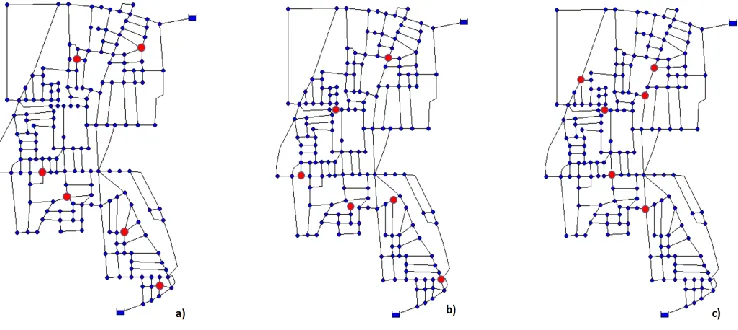
Figure 1: Sensor placement for the WDN of Parete: a) according to the un-weighted eigenvector centrality (EvC-1); b) according to the d/l weighted eigenvector centrality (EvC-2); c) according to the bi-objective

optimization (BOP)

head of 110 m a.s.l. Reference was made to the day of maximum consumption in the year with a total demand from the nodes ranges from 7.6 L/s (at night time) to 77.2 L/s (in the morning). It is fixed a total working number of 6 sensors to be placed in the water network. Three sensor layouts for Parete’s WDN are shown in Figure 1, corresponding to the un-weighted eigenvector centrality (EvC-1), d/l

weighted eigenvector centrality (EvC-2), and the BOP approach. An important aspect to highlight is that both the solutions obtained with the eigenvector centrality locates more sensors in the bottom part of the network; it is due to the greater difference in connection density which has led to a greater number of clusters (four clusters) in that area and so a greater number of sensors (four sensors). It is worth to note that, for the EvC-2 and the BOP solutions, one of the six sensors is located in the same node and two of them are located in the same close areas. It is the reason why, the simulation results are quite similar also in terms of detection time and detection likelihood, as it is shown in Table 1.

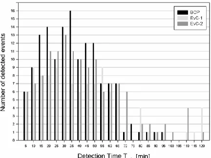
The time reporting step was set to 5 minutes in EPANET [27], and so, each event was detected in a time period multiple of 5 minutes. For each period, ranging from 5 to 120 minutes, the number of the detected contamination events is reported in Figure 2. In this regard, in Figure 2, the detection time for the all detected contamination events S and for the three procedures (respectively BOP, EvC-1, and EvC-2) are shown.

Figure 2: Detection time for all the detected events for the three sensor layouts, BOP, EvC-1, and EvC-2

The trends of the EvC-1 are more uniform than that of the EvC-2 and BOP, for which it is possible to define a clear mean value. It is also evident that, while the maximum detection time for the BOP is Tmin,max=95 min, for both EvC-1 and EvC-2, Tmin,max=120 min. In this regard, that means that, a small percentage of contamination events were detected with a delay of maximum 25 min.

Obviously the minimum detection time is Tmin,max=5 min for the three sensor layout, and it happens when the contamination event starts in correspondence of the nodes where the sensors are located. Regarding the mean value of the detection time, which more representative of the characteristic functioning of sensor system, for the EvC-1 Tmin,mean is equal to 42.4 min, for the EvC-2

Tmin,mean is equal to 42.2 min and for BOP Tmin,mean is equal to 36.1 min, which means that on average, the solutions provided using the eigenvector centrality (both un-weighted and d/l weighted) detect the contamination events with a delay of just 6 min. Finally, an important aspect to take into account for the water quality sensor monitoring systems is the percentage of the events that can be detect with respect to the whole set S of the considered contamination events. It is important to note that, EvC-1

confirm the efficiency of the proposed procedure in particular when the graph is weighted with d/l

which is related to the hydraulic conductivity of the pipes. In this way, it is possible to take into account not only the most linked nodes, but also the most important nodes which are crossed by the most conductive pipes.

Layout Tmin,min

[min]

Tmin,mean

[min]

Tmin,max

[min] Ps

[%]

EvC-1 5.0 42.4 120.0 56.1

EvC-1 5.0 42.2 120.0 73.1

BOP 5.0 36.1 95.0 78.2

Table 1: Minimum Tmin,min, mean Tmin,mean and maximum Tmin,max detection time and detection likelihood PS

for the three sensor layouts of Parete’s WDN

4

Conclusion

The work described in this paper uses a novel method to solve the problem of finding the optimal location for placing sensors in a WDN. This is by understanding a monitoring system is more efficient as it maximizes the possibility to cover a great area while minimizes, i.e., any event detection time and the number of sensor stations. The proposal adapts Complex Network Theory to sensor location in correspondence to the most important WDN nodes. In this regard, by exploiting the properties of the spectrum of the Adjacency matrix (or the weighted Adjacency matrix if the geometric information of the network is available), it is possible to define the eigenvector centrality. This attributes to each node a score equal to the corresponding coordinates of the principal eigenvector. The main advantage of this procedure relies on that it is not necessary to carry out hydraulic simulation or heuristic algorithms to analyze all the possible sensor placement layouts. It is worth to highlight that, exploiting the spectral properties of the WDN Adjacency matrix, it is also possible to reduce the space solutions and, consequently, the computational complexity of the optimization procedures, focus investigating nodes to place sensors to only a set of the most central nodes defined by the eigenvector centrality.

The overall procedure could be possibly being adapted to several aims by weighting the WDN graph with tailored weights according to each monitoring goal. Further work will investigate the possibility to define these weights to improve the results, testing the proposed procedure on larger WDNs and targeting other monitoring aims.

References

[1] O. Giustolisi and D. Savic, Identification of segments and optimal isolation valve system design in water distribution networks, Urban Water Journal, 7 (2010), 1–15.

[2] B.H. Lee and R.A Deininger, Optimal locations of monitoring stations in water distribution systems, J. Environ. Eng. 1992, 118 (1), 4-16.

[3] A. Kumar, M.L. Kansal, G. Arora, Identification of monitoring stations in water distribution system, J. Environ. Eng. 1997, 123 (8), 746-752.

[4] H.M. Woo, J.H. Yoon, D.Y. Choi, Optimal monitoring sites based on water quality and quantity in water distribution systems, In: World Water and Environmental Resources Congress, CD-ROM, ASCE, Reston, Va., 2001.

[5] A. Ostfeld and E. Salomons, Optimal layout of early warning detection stations for water distribution systems security, J. Water Resour. Plann. Manage., 2004, 130(5), 377–385.

[7] N Cheifetz, A.C. Sandraza, C. Feliers, D. Gilbert, O. Piller, A. Lang, An Incremental Sensor Placement Optimization in a Large Real-World Water System." Proc. Eng. 119(2015), 947–952.

[8] A. Ostfeld and E. Salomons, Sensor network design proposal for the battle of the water sensor networks (BWSN), Proc., 8th Annual Water Distribution System Analysis Symp., Cincinnati, 2006.

[9] G. Dorini, P. Jonkergouw, Z. Kapelan, F. Di Pierro, S.T. Khu, D. Savic, An efficient algorithm for sensor placement inwater distribution systems, In: Proc., 8th Annual Water Distribution Systems Analysis Symp., ASCE, Reston, Va., 2006

[10] J. Huang, E.A. McBean, W. James, Multiobjective optimization for monitoring sensor placement in water distribution systems, Proc., 8th Annual WDSA Symp., Cincinnati, 2006.

[11] Z.Y. Wu and T. Walski, Multiobjective optimization of sensor placement in water distribution systems, Proc., 8th Annual Water Distribution System Analysis Symp., Cincinnati, 2006.

[12] A. Preis and A. Ostfeld, Multiobjective contaminant sensor network design for water distribution systems." J. Water Resour. Plann. Manag., 2008, 134 (4), 366.

[13] S. Tinelli, E. Creaco, C. Ciaponi, Sampling significant contamination events for optimal sensor placement in water distribution systems, J. Water Res. Pl. Manag., 143(9), 2017.

[14] L. Perelman and A. Ostfeld, Topological clustering for water distribution systems analysis. J. Env. Soft. 26, 969-972, 2011.

[15] A. Yazdani, and P. Jeffrey, Complex network analysis of water distribution systems. An interdisciplinary journal of nonlinear science Chaos, 21(2011), 016111

[16] A. Di Nardo, M. Di Natale, C. Giudicianni, R. Greco, G.F. Santonastaso, Complex network and fractal theory for the assessment of water distribution network resilience to pipe failures. Water Science & Technology: Water Supply, July, 2017, DOI: 10.2166/ws.2017.124.

[17] M. Herrera, S. Canu, A. Karatzoglou, R. Pérez-García, J. Izquierdo, An approach to water supply clusters by semi-supervised learning, International Congress on Environmental Modelling and Software (2010), 1925-1932.

[18] A. Di Nardo, M. Di Natale, C. Giudicianni, R. Greco, G.F. Santonastaso, Water supply network partitioning based on weighted spectral clustering. Complex Networks & Their Applications V, Studies in Computational Intelligence; 693(2016), 797–807.

[19] B. Arsic, D. Cvetkovic, S.K. Simic, M. Skaric, Graph Spectral Techniques in Computer Sciences, Applicable Analysis and Discrete Mathematics, 6 (2012), 1– 30.

[20] F. Chung, Spectral graph theory, CBMS Regional Conference Series in Mathematics, Conference Board of the Mathematical Sciences, vol. 92, Washington, 1997.

[21] D. Cvetkovic and S.K. Simić, Graph spectra in computer science, Linear Algebra Appl., 434 (2011), 1545– 1562.

[22] P. Bonacich, Power and centrality: A family of measures. Am. J. Soc., 92 (1987) 1170–1182. [23] T. H. Wei, The algebraic foundations of ranking theory. Thesis, Cambridge 1952.

[24] L. Donetti, F. Neri, M.A. Munoz, Optimal network topologies: expanders, cages, ramanujan graphs, entangled networks and all that, Journal of Statistical Mechanics, (2006) P08007.

[25] B. Mohar, The Laplacian spectrum of graphs. In Graph Theory, Combinatorics, and Applications; Wiley: Hoboken, NJ, USA, 1991; pp. 871–898.

[26] J. Shi and J. Malik, Normalized cuts and image segmentation. IEEE Trans. Pattern Anal. Mach. Intell. 2000, 22, 888–905.

[27] L.A. Rossman, EPANET 2.00.10, United States Environmental Protection Agency (USEPA), Washington, D.C., EPA/600/R-00/057, https://www.epa.gov/water-research/epanet, 2000.

[28] A. Di Nardo, C. Giudicianni, R. Greco, M. Herrera, G.F. Santonastaso, Applications of Graph Spectral Techniques to Water Distribution Network Management, Water, 10(1), 45, 2018.

[29] A. Di Nardo, M. Di Natale, C. Giudicianni, D. Savic, Simplified Approach to Water Distribution System Management Via Identification of a Primary Network, Journal of Water Resources Planning and Management, DOI:10.1061/(ASCE)WR.1943-5452.0000885, 2017.