0 INTRODUCTION
Many authors have reported different methods of measuring and processing the captured Barkhausen noise (BN) voltage signals in their research.
Jiles and Suominen [1] found that micro-hardness and residual stresses were determined from the captured voltage signal of Barkhausen noise according to the measured depth. They found that at the same analyzing frequency and given specific electric conductivity and relative permeability of the material, a smaller depth of the micro magnetic change was obtained and vice versa. Wojtas and Suominen [2] and [3] stated that the X-ray measurement method is a reliable method for residual stress characterization, but it is slow and appropriate only for laboratory conditions. On the other hand, the magnetic Barkhausen noise (MBN) technique is fast and based on calibration curves for the determination of residual
stresses. Savaş and Gür [4] studied non-destructive
evaluation of surface residual stresses in shot peened steel components using the magnetic Barkhausen noise method. For this purpose, various sets of steel specimens were prepared by a controlled shot peening process with different intensities, impact angles and coverage values. The measurements showed that a clear relationship exists between surface residual
stresses and the Barkhausen noise signals. Grum and Žerovnik [5] also assessed the residual stresses in
steel 1C40 that had been hardened and tempered. The
assessment of the efficiency of the determination of residual stresses by the micro-magnetic method based on the BN was carried out by means of measurement of residual stresses using the relaxation method. Comparative through-thickness measurements showed that the micro-magnetic method was suitable for the determination of residual stresses since it gives a real-time variation of residual stresses in a thin surface layer of the material concerned in a very short
time. Žerovnik et al. [6] assessed the microstructure,
hardness, and residual stresses on induction surface-hardened specimens.
The most commonly chosen feature of the BN is the square mean value of the voltage signal
V2RMS. Desvaux et al. [7] studied ultrasonic shot
peening, which allows for control of the introduction of residual stresses on the raceways and increases the fatigue resistance of the bearings. The level of residual stresses that are introduced can be verified by BN at any point on the bearing raceway surface and
subsurface and guaranteed to 100% on a complete
manufacturing lot. Kikuchi et al. [8] determined the magnetic BN energy and the peak in the V2RMS voltage signal reflects the number of pinning sites for domain wall motion. These therefore rise sharply in an initial stage of cold rolling and almost saturate at a higher reduction ratio. On the contrary, the coercive force
and the magnetizing current at the peak in the V2RMS
Surface Integrity Characterization Based on Time-Delay of the
Magnetic Barkhausen Noise Voltage Signal
Žerovnik, P. – Fefer, D. – Grum, J.
Pavel Žerovnik1 – Dušan Fefer2 – Janez Grum1,*
1 University of Ljubljana, Faculty of Mechanical Engineering, Slovenia 2 University of Ljubljana, Faculty of Electrical Engineering, Slovenia
The captured magnetic Barkhausen noise (BN) signal is composed of a series of voltage impulses changes produced by movements of the magnetic domains. In most cases the captured voltage signals cannot be directly related to individual parameters to assess the material state, i.e. the properties, of the surface layer. For further efficient analysis of the voltage signals, an appropriate method for signal processing should be chosen in order to use the characteristic value of the voltage signal.
Our method of processing represents the time delay of a BN voltage signal, i.e. the maximum voltage value of the signal, with reference to the sine wave of the magnetizing current. Measurement of the time delays of the voltage signals was carried out under optimum magnetizing conditions, which gave us the greatest number of voltage impulses in the signal. These are influenced by the turns and orientation of the magnetic domains.
The aim of this research was to compare the voltage-signal time delay obtained with quenched and tempered specimens at two
neighbouring temperatures. The temperature differences ranged from ∆T1 = 10 °C, up to ∆T2 = 25 °C. These small temperature differences in
the tempering-temperature produced small differences in the micro hardness of the individual specimens and found out whether there were significant differences between micro hardnesses. The assessment of the reliability of the prediction of micro hardness was carried out using the Student’s t-test.
voltage increase monotonically due to the increase in
dislocation density below 10% and the formation of the cell structure. Žerovnik and Grum [9] discovered
that the microstructure and micro hardness have a significant effect on the relative permeability µr and
measurement depth z. The results showed that the
damping of the micro magnetic parameter with depth reaches its maximum in the soft specimen, and vice
versa. Lo et al. [10] studied the effects of
micro-structural variations with depth on the Barkhausen effect (BE) signals in surface-modified ferrous materials through measurements and simulations based on a hysteretic-stochastic model. Theoretical analysis showed that the model parameters, which describe the domain-wall pinning strength and the range of interaction of a domain wall with pinning
sites, are related to each other. Pepelnjak and Barišič
[11] have measured the strains occurring during sheet material plastic deformation using an optical measurement system. The strains were measured up to the tearing limit in order to determine the forming limit diagram using the Marciniak testing method. Due to the plane strain problem and fixing the focus distance between the observed sheet metal surface and the lens, only one charge-coupled device (CCD) camera was used. Sablik et al. [12] presented one model of the effect of plastic deformation on magnetoacoustic emission (MAE), where one must
first treat the non-180deg domain wall motion. In this
paper, they take the Alessandro-Beatrice-Bertotti-Montorsi (ABBM) model and modify it to treat
non-180deg wall motion. They then insert a modified
stress-dependent Jiles-Atherton model, which treats plastic deformation, into the modified ABBM model to treat MAE and MBN. An experimental study by
Vashista and Paul [13] was undertaken to investigate
the role of process parameters on the grindability of medium carbon steel in a high-speed grinding domain with particular emphasis on surface integrity. Surface residual stress on the ground specimens has been assessed using X-ray diffraction techniques and BN analysis. High-speed grinding with cubic boron nitride (CBN) wheels, unlike conventional grinding, provided compressive residual stress throughout the experimental domain. This can be attributed to the desirable temperature control since the single layer CBN wheel had higher thermal conductivity than conventional wheels and grinding fluid took away a substantial part of the grinding heat flux. Micromagnetic or BN parameters correlated linearly with the residual stress, indicating its applicability in assessing the surface integrity of high-speed ground
steel. Koomatsubara et al. [14] captured the BN of soft
ferrites and silicon steels. The experimental data are discussed in terms of the relevant quantities: saturation flux density (Bs), conductivity sigma, cross-sectional area of samples (SO) and grain diameter (d). At low
field velocities mod (H), magnetization processes
are dominated by independent displacements of 180
degrees walls. The peak noise power (Pm) in the
vicinity of the coercive field is proportional to the
field velocity mod (H) mod. These two simple results
reflect nonoverlapping Barkhausen pulses. Krause et
al. [15] compares the anisotropy of surface MBN and
the pulse height distributions between two samples
of oriented 3% Si-Fe steel laminate at equivalent
flux densities. Differences between the two samples were observed in the anisotropic behavior of the MBN-Energy and pulse height distributions for flux
density amplitudes between 1.3 and 1.6 T, the typical
operating range of transformer laminates. These were attributed to differences in the number and structure of
the 180° domain walls. Schneider et al. [16] studied
the surface acoustic waves as a means of evaluating surface-hardened steels. A generalized dispersion curve was calculated using the theory of the surface acoustic wave to deduce the hardening depth from the velocity. Using this methodology, it was found that the hardening depth could be determined with an error not
higher than 15%.
1 EXPERIMENTAL SET-UP
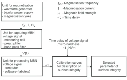
For these investigations an experimental setup was arranged to capture voltage signals of the MBN.
It consisted of a magnetisation unit, a sensor for
capturing voltage signals, a signal amplifier with a relevant band-pass filter, and a computer-aided unit for determination of the microstructure or micro hardness and residual stresses. Fig. 1 shows a block scheme of the experimental setup for micromagnetic testing based on the BN.
In the analysis of the BN at the chosen depth,
it was important to filter the BN voltage signals. A frequency filter provided a signal of the voltage induced in the measuring coil sensing the changes during the process of specimen magnetization. Thus a Butterworth filter of the fourth order was applied in a series connection with a low-pass and high-pass filter of the second order. Thus, in the experimental setup, four different band-pass Butterworth filters of the fourth order pass signals in different frequency ranges.
2 THE ANALYZED MATERIAL AND SELECTION OF OPTIMAL MAGNETIZING PARAMETERS
In our research, we used 1C55 heat-treated carbon steel with a 0.58% carbon content, which is used in
the production of various machine parts exposed to heavy loading.
Table 1. Chemical composition of steel 1C55 [wt.%]
C Si Mn Cr Ni Cu Al Sn Mo V Ti
0.58 0.26 0.63 0.10 0.15 0.28 0.02 0.013 0.03 0.01 0.002
For this purpose, ferromagnetic steel bands of
150×30×5 mm were subjected to three types of heat
treatment:
• Soft-annealed specimens, annealed at a
temperature of TSA = 690 °C, with an average microhardness of 224 HV0.2.
• Specimens quenched in oil at a temperature of
TH = 850 °C, with an average micro hardness of 803 HV0.2.
• Specimens quenched in oil at a temperature of
TH = 850 °C, tempered to a temperature of TT = 300 °C, with an average micro hardness of 511 HV0.2.
After different heat treatments of steel 1C55 we
obtained different structural changes and different profiles of micro hardness.
At the soft annealed temperatures TSA = 690
°C, a fine pearlite-ferrite microstructure forms. The
size and density of the coagulated cementite in the pearlite grains determine steel hardness after heat treatment (Fig. 2a). The specimens quenched in oil at
a temperature of TH = 850 °C show a microstructure
of fine tetragonal martensite (Fig. 2b). With the specimens quenched in oil at a temperature of
TH = 850 °C and tempered to a temperature of TT = 300 °C, martensite will disintegrate into a bainite
microstructure. Thus, the bainite microstructure shows
very fine feathers of cementite in the ferritic matrix (Fig. 2c).
Fig. 2. The microstructure and micro hardness of individual heat-treated 1C55 steel specimens; a) soft annealed, b) quenched
in oil, c) quenched and tempered
Before initiating these experiments, it was necessary to select the optimum magnetization parameters. Various magnetization parameters affect the shape of the signals captured and the number of
voltage impulses in the signal. In the first phase, the
number of voltage impulses in the voltage signal was determined as a function of the magnetizing frequency (fe), and the magnetizing current (I). The experimental work accomplished hitherto indicates that voltage signals having a higher density of voltage impulses provide more useful data on the material.
Fig. 3. Density of voltage impulses in the signal as a function of
the magnetizing frequency and constant magnetizing current
The Barkhausen voltage signals were captured
TSA of 690 °C. Fig. 3 shows the number of voltage
impulses in the signal as a function of the magnetizing
frequency and a constant magnetizing current. Fig. 4
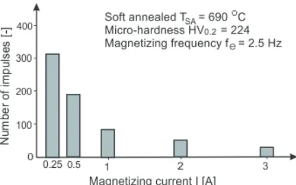
shows the number of voltage impulses in the signal as a function of the magnetizing current and a constant magnetizing frequency.
The diagrams in Figs. 3 and 4 indicate that the
density of impulses in the voltage signal is reduced if the magnetizing frequency and the magnetizing current increase and vice versa.
Fig. 4. Density of voltage impulses in the signal as a function of
the magnetizing current and constant magnetizing frequency
3 PROCESSING THE BN VOLTAGE SIGNAL ON THE BASIS OF TIME DELAYS
The captured BN voltage signal is composed of a
series of voltage impulses. In the first phase the
voltage impulses rise as they near the centre of the voltage signal and then decrease in the same manner toward zero. Changes in voltage impulses are caused by the movements of magnetic domains. The whole
captured voltage signal of an MBN is unstationary. In
limited parts of the voltage signal the stationary can be defined as stationary in the narrow or the wide
part of the signal. In the central part of the captured
voltage signal we can assume the stationary in wide range. This means that when evaluating the voltage signal it is sufficient that the first two central moments (arithmetic mean of the signal mx2 and signal variance
σ2)are time independent.
In most cases the captured voltage signals cannot
be directly related to individual parameters to assess the state, i.e. properties, of the surface layer. For further efficient analysis of the voltage signals, an appropriate method for signal processing should be chosen in order to use the characteristic value of the voltage signal.
In the analysis of the captured voltage BN
signals we noticed various time delays according to
the sinusoidal of the magnetizing current. In the first
phase, we sketched out an envelope of the captured voltage signal of BN. The time delay was measured from the highest point of the envelope (which also represents the area with the highest voltage impulses) to the sinusoidal of magnetizing current, as shown in
Fig. 5.
Fig. 5. Definition of the time delay of the BN voltage signal with
reference to the sinusoidal of the magnetizing current
We found that different magnetizing parameters, as the current of the material, affected the size of
the time delays. In the analysis of the magnetizing
parameters we focused on the two most important
ones, which were the magnetizing current I and the
magnetizing frequency fe. The current of the material
is affected by heat treatment with consequent changes in microstructure and hardness, in the mechanical treatment with cutting, on the level of plastic deformation and so on.
The plot of the envelope of the voltage signal and the measurement of time delays from the sinusoidal of the magnetizing current were carried out with computer aid.
3.1 The Influence of Various Magnetizing Parameters on
the Time Delays of BN Signals
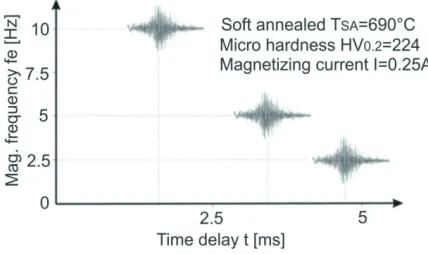
Figs. 6 and 7 show the time delays of the voltage
signals with different magnetization parameters. We need to change both the magnetizing current and the magnetizing frequency fe. Fig. 6 shows the time delay
of the signals captured with different magnetizing current intensities and a constant magnetizing frequency fe of 2.5 Hz. The longest time delays are obtained with the lowest magnetizing current intensities so that with a current intensity I of 0.25
A, the time delay t equals 4.70 ms. The shortest time
delay t, i.e. 0.80 ms, is obtained with a magnetizing
current I of 3 A.
frequencies produce shorter time delays so that with a frequency fe of 10 Hz a time delay t of 1.40 ms is
obtained whereas with a lower frequency fe, i.e. 2.5
Hz, the time delay t of the signal is considerably
longer, i.e. 4.70 ms.
Fig. 6. Variation in the time delays of the maximum voltage
values of BN signals as a function of different magnetizing current intensities and constant magnetizing frequency
Fig. 7. Variation of time delays of the maximum amplitude values
of BN signals as a function of different magnetizing frequencies and constant magnetizing current
3.2 The Influence of Heat Treatment on the Time Delay of Voltage Signals
We continued our research with the measurement of time delays of voltage signals. The measurements were performed on specimens that were heat treated with consequent change in microstructure and micro hardness (Fig. 2).
Measurement of the time delays of the voltage signals was carried out under optimum magnetization conditions. The optimum magnetization conditions are the ones giving the highest number of voltage impulses in the signal. They are influenced by the turns and orientation of the magnetic domains. Based on the given criteria related to the density of impulses in the BN voltage signal and the length of time delays of the signal, it can be stated that:
• the highest density of voltage impulses is obtained
with a magnetizing frequency f of 2.5 Hz and a
magnetizing current I of 0.25 A and
• the longest time delays t, i.e. 4.70 ms, are obtained
with a magnetizing frequency f of 2.5 Hz and a
magnetizing current I of 0.25 A (to a specimen in
the soft annealed state).
Data on time delays of the voltage signals, including the calculated mean values and data on microhardness are given in Table 2. The data indicate that there are differences in the time delays of the individual specimens in different states. For the specimens with higher hardness, a longer time delay is obtained and vice versa.
Table 2. Mean values of the time delays of the voltage signals with data on microhardness for the individual heat treated specimens
Heat treatments Micro hardnessHV
0.2
Time delays (mean values) t [ms]
Quenched, TH = 850 ºC 803 13.1
Quenched and tempering
TH = 850 ºC, TT = 300 ºC 511 9.3
Soft annealed, TSA = 690 ºC 224 4.7
Fig. 8 shows microhardness HV0.2 of the
specimens in three different states as a function of time delays of the voltage signals.
Fig. 8. Microhardness as a function of time delays from specimens of steel 1C55 in three different states
Results of the statistical analysis between the time delays of the voltage signals and the corresponding hardness are very favourable since the calculated correlation coefficient rt/HV is equal to 0.989.
4 DETERMINATION OF THE MICRO HARDNESS AND RELIABILITY ASSESSMENT
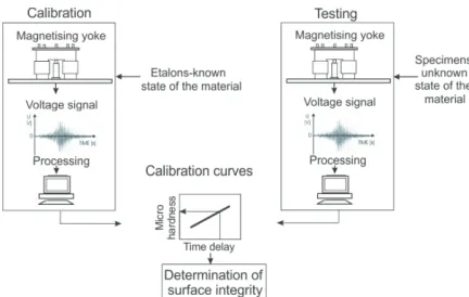
followed by measurements, and later a classification of the specimens with an unknown state. The calibration procedure and determination of micro hardness by
means of the calibration curve is shown in Fig. 9. The left part of Fig. 9 shows the procedure for
elaborating the calibration curves using etalons with a known micro hardness, whereas the right part shows the procedure for testing an unknown specimen, i.e. determination of the characteristics of the surface-hardened layers.
The time delay was measured from the highest point of the envelope (which also represents the area with the highest voltage impulses) to the sinusoidal of the magnetizing current. The plot of the envelope of voltage signal and the measurement of time delays from sinusoidal of magnetizing current were carried out with computer aid. The data indicate that there are differences in the time delays of the individual specimens in different states. For the specimens with higher hardness, a longer time delay is obtained and vice versa. The following findings can be stated:
• When measuring specimens with an unknown
micro hardness or unknown specimens, a suitable calibration curve determined on the basis of a preliminary measured micro hardness after heat treatment should be selected;
• A suitable calibration curve having been selected,
measurement is carried out on the specimens with an unknown micro hardness. The time delays are then measured. By means of the calibration curve, the corresponding micro hardness value is determined.
The analysis of the results obtained made it possible to determine the reliability of the assessment of micro hardness of a given specimen based on the time delay of the voltage signal captured. The assessment of the reliability of predicting micro hardness was carried out using the Student’s t-test.
Micro hardness measurement reliability analysis was conducted on the hardened and tempered specimens. For each high-tempering temperature three specimens were available. Three measurements were taken for each specimen, which means that nine measurements at the same tempering temperature were performed.
The aim of the research was to compare the voltage-signal time delay obtained with the quenched and tempered specimens at two neighbouring temperatures. The temperature differences ranged from ∆T1 = 10 °C, up to ∆T2 = 25 °C. The second aim of the research was to distinguish small differences in the micro hardness of the two neighbouring specimens
and to find out whether there were significant differences.
Fig. 9. Determination of micro hardness by means of calibration
curves
In the study the quenched and tempered
specimens tempered from TT1 = 300 °C to TT5 = 400
°C were used. Four different tempering temperatures rising gradually by 25 °C were chosen.
Fig. 10 shows envelopes of the voltage signals
captured from the samples in different states. The first envelope with a time delay t = 4.85 ms belongs to
the quenched specimen in oil from TH = 850 °C and
with the tempering temperature TT = 400 °C. The last
envelope with a time delay t = 9.30 ms belongs to the
quenched specimen in oil from TH = 850 °C and with
the tempering temperature TT = 300 °C.
The harder specimens show a lower and flatter envelope with a longer time delay with regard to the sinusoidal of the magnetizing current and vice versa.
Fig. 10. Voltage signal envelopes for quenched and tempered
specimens at different temperature
In Table 3 the comparative results of the
individual tempering temperatures. All of the first four results of significance were lower than the chosen
limit of confidence (0.00092; 0.00038; 0.00004; 0.00001 < 0.05), which indicates that a hypothesis
on the equality of the micro hardness among the tempering temperatures chosen was rejected and there were significant differences between the micro hardness chosen.
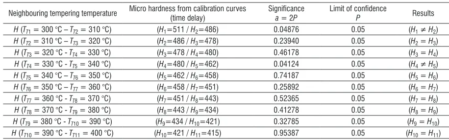
In Table 4 comparative results of micro hardness
significance are given for neighbouring tempering-temperature pairs. Tempering tempering-temperatures rose
gradually by 10 °C between two neighbouring
specimens. Most of the results of significance in Table
4 were higher than the chosen limit of confidence,
which means that the differences in the micro hardness between the two neighbouring specimens were insignificant.
5 CONCLUSION
The time delays are defined between the sinusoidal of the magnetizing current and the maximum amplitudes of the BN voltage signals. Statistical analysis was applied to the assessment of the reliability of micro hardness prediction, based on the time delays of the voltage signals. The aim of the research was to produce small differences in micro hardness of the individual specimens and to find out whether
there were significant differences. In addition to the
assessment of reliability the power of the statistical
relationship between the time delays and micro hardness in the entire tempering-temperature range was assessed.
The statistical analysis provided the following findings:
• The time delays of the captured BN voltage signal
is a good estimator of the micro hardness of the
1C55 heat-treated carbon steel, which is indicated
by the high values of the calculated correlation coefficients (rt˝/HV0.2 = 0.989).
• The temperature differences ranging by ∆T2 =
25 °C give us significant differences in micro
hardnesses, determined from the time delays, between neighbouring tempering-temperature pairs.
• The temperature differences ranging by ∆T1 =
10 °C show mostly insignificant differences in
micro hardnesses, determined from time delays, between neighbouring tempering-temperature pairs.
• The results of the micro hardness assessed from
the time delay of the BN differ from the average
by 16 HV from the measured Vickers hardness.
We estimated that this new micro magnetic method of signal processing is fast, reliable, repeatable and represents a successful estimator for determining
the micro hardness of the steel 1C55 in different states. Table 3. Test of micro hardness significance for different neighbouring tempering-temperature pairs (∆T2 = 25 °C)
Neighbouring tempering temperature Micro hardness from calibration curves
(time delay)
Significance
a = 2P Limit of confidence P Results
(TT1 = 300 °C to TT2 = 325 °C) (H1 = 511 / H2 = 482) 0.000924 0.05 (H1 ≠ H2)
(TT2 = 325 °C to TT3 = 350 °C) (H2=482 / H3 = 464) 0.000382 0.05 (H2 ≠ H3)
(TT3 = 350 °C to TT4 = 375 °C) (H3 = 464 / H4 = 439) 0.000049 0.05 (H3 ≠ H4)
(TT4 = 375 °C to TT5 = 400 °C) (H4 = 439 / H5 = 415) 0.000013 0.05 (H4 ≠ H5)
Table 4. Comparative results of micro hardness significance for neighbouring tempering-temperature pairs (∆T1 = 10 °C)
Neighbouring tempering temperature Micro hardness from calibration curves (time delay) Significance a = 2P Limit of confidenceP Results
H (TT1 = 300 °C – TT2 = 310 °C) (H1=511 / H2=486) 0.04876 0.05 (H1 ≠ H2)
H (TT2 = 310 °C – TT3 = 320 °C) (H2=486 / H3=478) 0.23940 0.05 (H2 = H3)
H (TT3 = 320 °C - TT4 = 330 °C) (H3=478 / H4=480) 0.46178 0.05 (H3 = H4)
H (TT4 = 330 °C - TT5 = 340 °C) (H4=480 / H5=462) 0.04124 0.05 (H4 ≠ H5)
H (TT5 = 340 °C – TT6 = 350 °C) (H5=462 / H6=458) 0.74187 0.05 (H5 = H6)
H (TT6 = 350 °C – TT7 = 360 °C) (H6=458 / H7=451) 0.25892 0.05 (H6 = H7)
H (TT7 = 360 °C - TT8 = 370 °C) (H7=451 / H8=443) 0.52365 0.05 (H7 = H8)
H (TT8 = 370 °C - TT9 = 380 °C) (H8=443 / H9=434) 0.41278 0.05 (H8 = H9)
H (TT9 = 380 °C - TT10 = 390 °C) (H9=434 / H10=421) 0.32785 0.05 (H9 = H10)
6 REFERENCES
[1] Jiles, D.C., Suominen, S. (1994). Effects of surface
stress on barkhausen emissions, model predictions
and comparison with X–ray diffraction studies. IEEE
Transactions on Magnetics, vol. 30, no. 6, p.
4924-4926, DOI:10.1109/20.334267.
[2] Wojtas, A. (2004). Surface and subsurface
residual-stresses after shot peening-their qualitative and quantitative analysis by X-Ray diffraction and Barkhausen noise analysis. Metal Finishing News, Wetzikon.
[3] Suominen, L., Tiitto, K. (1994). Use of X-ray diffraction
and Barkhausen noise for the evaluation of stresses in shot peening. Proceedings of 4th International
Conference on Residual Stresses, Baltimore, p.
443-448.
[4] Savaş, S., Gür, H. (2010). Monitoring variation
of surface residual-stresses in shot peened steel components by the magnetic Barkhausen noise method.
Insight, vol. 52, no. 12, p. 672-677.
[5] Grum, J., Žerovnik, P. (2000). Use of the Barkhausen
Effect in the Measurement of Residual Stresses in Steel. Insight, vol. 42, no. 12, p. 796-800.
[6] Žerovnik, P., Grum, J., Žerovnik, G. (2010).
Determination of hardness and residual-stress variations in hardened surface layers with magnetic barkhausen noise. IEEE Transactions on Magnetics, vol. 46, no. 3, p. 3221-3224, DOI:10.1109/TMAG.2009.2032417.
[7] Desvaux, S., Gualandri, J., Carrerot, H. Lamare, A. (2003). Industrial application process of impruvement of the high precision bearings service life –
pre-stress, Barkhausen noise. International Conference on Barkhausen Noise and Micromagnetic Testing ICBM, p. 49-62.
[8] Kikuchi, H., Ara, K., Kamada, Y., Kobayashi, S. (2009).
Effect of microstructure changes on Barkhausen noise properties and hysteresis loop in cold rolled low carbon steel. IEEE Transactions on Magnetics, vol. 45, no. 6, p. 2744-2747, DOI:10.1109/TMAG.2009.2020545.
[9] Žerovnik, P., Grum, J. (2009). Determination of residual
stresses from the Barkhausen noise voltage signal, 10th
International Conference of the Slovenian Society for
Non-Destructive Testing, Ljubljana, p. 437-445.
[10] Lo, C.C.H., Kinser, E. R., Jiles, D.C. (2006). Analysis
of barkhausen effect signals in surface - modified magnetic materials using a hysteretic-stochastic model. Journal of Applied Physics, art. no. 08B705, DOI:10.1063/1.2163272.
[11] Pepelnjak, T., Barisic, B. (2009). Computer-assisted
engineering determination of the formability limit for thin sheet metals by a modified Marciniak method.
Journal of Strain Analysis, vol. 44, no. 6, p. 459-472,
DOI:10.1243/03093247JSA503.
[12] Sablik, M.J., Augustyniak, B., de Campos, M.F.,
Landgraf, F. (2008). Modeling of effect of plastic
deformation on Barkhausen noise and magnetoacoustic
emission in iron with 2% silicon. IEEE Transactions on
Magnetics,vol. 44, no. 1, p. 3221-3224, DOI:10.1109/
TMAG.2008.2002803.
[13] Vashista, M., Paul, S. (2008). Study of the effect of
process parameters in high-speed grinding on surface integrity by Barkhausen noise analysis. Journal of
Engineering Manufacture, vol. 222, no. 12, p.
1625-1637, DOI:10.1243/09544054JEM1214.
[14] Koomatsubara, M., Porteseil, J.L., Nakamura, H. (1988). Comparison of Barkhausen noise power
between soft ferrites and silicon steels. IEEE
Transactions on Magnetics, vol. 24, no. 2, p.
1704-1706, DOI:10.1109/20.11576.
[15] Krause, T.W., Szpunar, J.A., Atherton, D.L. (2003).
Anisotropic flux density dependence of magnetic
Barkhausen noise in oriented 3% Si-Fe steel laminates.
IEEE Transactions on Magnetics, vol. 44, no. 1, p.
562-566, DOI:10.1109/TMAG.2002.806352.
[16] Schneider, D., Hofmann, R., Schwarz, T., Grosser, T., Hensel, E. (2012). Evaluating surface hardened
steels by laser-acoustics. Surface & Coatings
Technology, vol. 206, p. 2079-2088, DOI:10.1016/j.
![Table 1. Chemical composition of steel 1C55 [wt.%]](https://thumb-us.123doks.com/thumbv2/123dok_us/8950816.1860184/3.598.332.514.119.328/table-chemical-composition-steel-c-wt.webp)