Volume 22 - Article 4 | Pages 95–114

in the population sciences published by the Max Planck Institute for Demographic Research Konrad-Zuse Str. 1, D-18057 Rostock · GERMANY www.demographic-research.org

DEMOGRAPHIC RESEARCH

VOLUME 22, ARTICLE 4, PAGES 95-114

PUBLISHED 19 JANUARY 2010

http://www.demographic-research.org/Volumes/Vol22/4/ DOI: 10.4054/DemRes.2010.22.4

Research Article

The negative educational gradients

in Romanian fertility

Cornelia Mureşan

Jan M. Hoem

© 2010 Cornelia Mureşan & Jan M. Hoem.

This open-access work is published under the terms of the Creative Commons Attribution NonCommercial License 2.0 Germany, which permits use, reproduction & distribution in any medium for non-commercial purposes, provided the original author(s) and source are given credit.

1 Introduction 96

2 Trends and patterns in Romanian cohort fertility 97

3 Period fertility: Data and method 98

4 Main finding: The negative educational gradient in parity-specific fertility

102

5 Possible explanations for the negative gradients 105

6 Acknowledgements 106

The negative educational gradients in Romanian fertility

Cornelia Mureşan1

Jan M. Hoem2

Abstract

In Western countries, rates of second and third births typically increase with educational attainment, a feature that usually disappears if unobserved heterogeneity is brought into the event-history analysis. By contrast, in a country like Romania, second and third birth rates have been found to decline when moving across groups with increasing education, and the decline becomes greater if unobserved heterogeneity is added to the analysis. The present paper demonstrates this pattern, and shows that, because this feature is retained in the presence of control variables, such as age at first birth and period effects, the selectivity is not produced by a failure to account for the control variables.

1. Introduction

In a tradition going back to the seminal book by Gary Becker (1981), economists typically hypothesize that fertility will decrease as women’s educational levels increase, because childbearing intensities are dominated by differential opportunity costs. A long string of demographic contributions have shown the opposite pattern for countries in the West, namely, that in the populations studied in recent years, more highly educated women have had higher fertility at parities above zero than women with less education (Kravdal 2001, Hoem et al. 2001, Kreyenfeld 2002, Oláh 2003, Kreyenfeld and Zabel 2005, Köppen 2006). The explanation often given for this positive educational gradient at positive parities found in Western data is that the more highly educated women who become mothers constitute a select group of particularly childbearing-prone3 _{women, a} development which should result in a reduction in the educational gradient at parities above zero when unobserved heterogeneity is brought into the picture. In fact, the gradient regularly disappears, i.e., it is essentially reduced to zero.

By contrast, a negative educational gradient has been found (as predicted by Becker’s theory) for some countries in Eastern Europe. (For Albania, see Gjonca et al. 2008, Fig. 4; for the Ukraine, see Perelli-Harris 2008, Figure 5; for an investigation with particularly clear results, see Koytcheva 2006, who studied patterns for first and second births in Bulgaria in her Chapter 6.) In the present paper, we use event-history analysis with a number of control variables to show that negative educational gradients in fertility are present for Romania for all birth orders one through three. We suggest that Romanian educational gradients may be negative precisely for the reasons given in the Beckerian theory (i.e., opportunity cost considerations and quantity-quality trade-off), as we have little reason to suspect that a strong income effect will be found, especially during the socialist period, when education did not play any important role in wage differentials. We speculate that the rapid increase in income dispersion during the subsequent market-oriented period produced a growth in the return to education, which was likely to increase the opportunity costs of childbearing, especially for better educated women. In addition, we suggest that women with higher levels of education must have been more successful in avoiding the coercive measures of the pronatalist policies in the socialist period (simply because they were more talented in adapting to the circumstances), and that (for the same reason) they benefited to a greater extent when more childbearing-friendly conditions appeared. The lower childbearing intensities among women with higher levels of education appear to have persisted over the entire period of investigation. In Romania, the educational gradients become even

3 _{This term encompasses the woman’s attitudes and values, and those of her partner if she has a partner, as}

more strongly negative when we control for unobserved personality characteristics. We suggest that the explanation may be the same as for Western countries: Women who become mothers are positively selected for childbearing-proneness, and, even though in Romania this selection is not strong enough to overcome other factors and produce a positive educational gradient, the gradient becomes smaller (in this case, more negative) when we account for unobserved heterogeneity. In this respect, Romania appears to be similar to other countries for which this issue has been studied.

In the present paper, we first display negative educational gradients in parity-progression rates for cohorts in the Romanian census of 2002. While these rates reflect the structure of women’s final parity at the end of childbearing, they do not reflect explicitly the childbearing dynamics that lead up to the end product, and the rates may therefore be confounded by changing age patterns and developing birth intervals. These issues are kept under control in hazard regression, the method we use for most of our analysis. The bulk of our paper is concerned with the pattern of educational attainment in relative risks of childbearing of birth orders one, two, and three. To avoid drawing attention away from this main topic, we relegate our results concerning other covariates to Appendix 2.

2. Trends and patterns in Romanian cohort fertility

Figure 1: Parity progression ratio (PPR), trend across birth cohorts, for each parity and educational level

0 10 20 30 40 50 60 70 80 90 100

1948-52 1953-57 1958-62 1963-67

Parity 0, no ed Parity 0, mid ed

Parity 0, hi ed Parity 1, no ed Parity 1, mid ed Parity 1, hi ed Parity 2, no ed

Parity 2, mid ed Parity 2, hi ed

3. Period fertility: Data and method

To get a more detailed picture of Romanian fertility trends and patterns, we have analyzed the data of the first round of the national Generations and Gender Survey (GGS), collected at the end of 2005.4 _{The sample consists of 11,986 respondents (5,977} men and 6,009 women) aged 18 to 79 at the time of interview, but our primary focus is on the 6,002 women who had proper childbearing and educational histories.5

4 _{The Romanian Generations and Gender Survey (GGS) was conducted within the framework of the}

international Generations and Gender Programme (GGP) with the financial support of the United Nation Fund for Population Activities (UNFPA) and the Max Planck Institute for Demographic Research (MPIDR). More details about the program can be found on the website of the Population Activities Unit of the United Nations Economic Commission for Europe (UNECE PAU), http://www.unece.org/pau/ggp, the coordinator of the whole project, and on the website of MPIDR, http://www.demogr.mpg.de.

5 _{We eliminated seven women: one for having an improper childbearing history, five for not having the}

In the GGS, respondents were asked to report the date (month and year) of each event. Consequently, our timing estimates have the precision of one month. We have imputed the middle of the month as the exact time of each birth, and made this our dependent variable.6 _{Mothers are not counted as exposed to risk until nine months after} the previous birth. We right-censored observations after 15 years, or when the woman reached age 40, or if she had not had another birth by the date of the interview.

1( )

i

h t

1( ) y t

1( )

ik

Our key explanatory variable is educational attainment. Unfortunately, we do not really have complete educational histories, as only the highest educational level at the time of interview and the year and month of completion are reported in the first-round GGS. We cannot use the final educational level as a time-constant covariate because the results would be strongly biased for several reasons which have been discussed, for example, by Kravdal (2004) or Hoem and Kreyenfeld (2006) in their papers about anticipatory analysis. We have chosen the same solution as the latter authors, namely, to impute a current educational level, which is time-varying, and the value of which changes when the respondent is deemed to have completed her final educational level.7 In addition to the three categories of low, middle, and high educational attainment, which we explained in Chapter 2 above, we have a separate category for women who are regarded as still participating in education in the current month. Details can be found in Appendix 1.

For first births, we apply a hazard regression model with an intensity , which for the ith _{woman has the form}

1 1 1 1 1 0

lnh ti ( )= y t( )+

∑

Here t is the process time, defined as her age (counted from age 12). The log-baseline intensity is represented as a linear spline function of t. Furthermore,

x t

1

exp( k )

is an indicator of whether she has reached educational level k at process time t, (including whether she is deemed to be in education at that process time), and

β is the relative risk of occurrence of a first birth for educational category k (with βk1=0 for k=1, say). Finally, a second piecewise linear spline is intended to capture the effect of calendar time (counted since the beginning of the year 1950). The argument is the calendar time at which we take individual i to start to be exposed to the risk of a first birth, i.e., the calendar month in which she turns 12. Thus

1 c z 0 i c

6 _{Instead of considering the time to each birth as our dependent variable and the exposure to risk since nine}

months after the previous birth, we might have considered the time to each conception (that ended in a live birth) as our dependent variable and the time at the last previous birth as the start of exposure to risk. Both strategies are equally good.

1950

2

a

z a1

1

i

c

2

i

c za3

0

i

c + −t

l

l

is the calendar month in which the respondent is 12+t years old, counted from the beginning of 1950.

For second births we use a corresponding specification

2 2 2 2 2 1 2 1

nh ti ( )= y t( )+

∑

where is another linear spline used to pick up the effect of the age at first birth (counted from age 18), and the other items are quite similar to those of the intensity of a first birth. Process time t is now months since first birth, and is the calendar month of the first birth. Note that the educational-level binaries vary by birth order because process time t differs from one birth order to the next.

We extend this specification to third births by using a parallel third-birth intensity of the form

3 3 3 3 3 2 3 1

nh ti ( )= y t( )+

∑

where is the calendar month of the second birth. Note that the spline is supposed to pick up the effect of the woman’s age at first (not second) birth on the third-birth intensity. We suppose that what is most important is the age at entry into motherhood, not the age at last previous birth.8

These specifications of {h til( );l=1, 2,3} are supposed to reflect the effects of the

observed covariates on the intensities when we do not account for unobserved factors, i.e., when we assume that all female respondents with the same values of {xikl( )}t

i

h_{l l}

0)

= va

, , , and so on have the same childbearing intensities, as specified. Alternatively, we may try to account for unobserved differences in the individual characteristics of the respondents. As usual among users of the software aML, we do this by adding an unobserved-heterogeneity factor to the above formula for ln (for each ), and by assuming that the triple is tri-normally distributed with a zero mean

for each , some set of variances

i

c_l

1 a

(EUil

i

U_l

1, 2, 3

{U U Ui i i }

l rUil=σl2, and correlations

'=correlation(Uil,Uil')forl l≠ '. (The triples are taken to be independent across

ρ_ll

8 _{Among demographers, this phenomenon is known as the “engine of fertility.” The metaphor reflects the idea}

'}

individuals i.) We would expect each correlation to be positive, as we assume that a woman who is unusually childbearing-prone, say, for the values that she has on the observed control variables, will be so across all birth orders. Note that we can specify that two of the unobserved-heterogeneity factors are identical by specifying that the corresponding correlation be identically 1 (for all individuals). For other correlations, the {ρ_ll are estimated along with the _{{ }σ}2

l when the model is fitted to the data.

It is worth mentioning that, while we would expect these general features of the heterogeneity specification to be shared by all populations, the heterogeneity parameters (i.e., the {σl} and the {ρll'}) must vary across populations, and therefore

need to be estimated for each population. It may be assumed that a population in which some 87% of all women become mothers (according to the Romanian GGS data from 2005 that we studied) must have selection mechanisms that are quite different from those of a population in which only around three-quarters of women have children (according to the German Family and Fertility Survey of 1992; see Hoem and Kreyenfeld 2006, Table 5). We trust that such differences will be reflected in notable differences in the heterogeneity parameters, and that these differentials suffice to account for the differences in selection mechanisms.9

We need to give some additional attention to the specification of the calendar-time splines . The defining items are the location of their nodes, which we have selected to reflect major political and institutional changes in Romanian society. The fall of the communist regime at the end of 1989 is an important node for our calendar, but there are also other breaks caused by major changes in social policy in recent Romanian history. For instance, there have been important changes in abortion legislation, and we want these changes to be reflected in our calendar splines. Abortion was legalized in 1957, and was widely used to limit family size. In 1967, abortion was suddenly banned, which resulted in a doubling of the number of births over the next three years. Abortion was again legalized in 1989, on the eve of the collapse of the old socio-political regime. There have also been other changes in family policy. The first forms of financial support for children were introduced in 1956, but a wide-ranging pronatalist policy was not implemented in Romania until 1967. The demographic policies of the “golden age” of Ceausescu’s regime lasted between 1967 and 1989. The emerging industry needed a growing work force, including working women, and the Romanian family policy was set and developed in those years with this in view. Incentives and coercive measures together resulted in more births of all orders, relative to the periods before 1967 or after 1989. Moreover, higher-order birth risks were very

{ }zcl

9 _{It might help if the form of the heterogeneity distribution were also allowed to vary across populations}

sensitive to periodic re-enforcements of pronatalist policies in June 1973 and March 1984. The birth rate declined every time the corps-control weakened, and it rose again when measures against illegal abortions were strengthened (Mureşan 1996, 2008). After 23 years of the authoritarian communist regime, 1990 marked the start of freedom and of a re-definition of family policies. One year of paid childcare leave for working mothers was introduced in 1990, and this was extended to two years in 1997. Paternity leave was introduced in 1999, childcare benefits for “insured” mothers in 2003, and a number of other incentives designed to increase the low level of fertility have since been introduced (Mureşan et al. 2008).

These considerations have led us to use the following nodes in the linear spline that represents our period function: start of 1950, start of 1967, end of 1969, mid-1973, mid-1974, mid-1984, mid-1985, start of 1990, start of 1997, start of 2003, and end of 2005.

For the baseline splines we located the nodes simply so they fit the data suitably after some experimentation, and we used the same practical criterion for the nodes of the splines that represent the effect of age at first birth. For details, see the tabulation in Appendix 2.

4. Main finding: The negative educational gradient in parity-specific

fertility

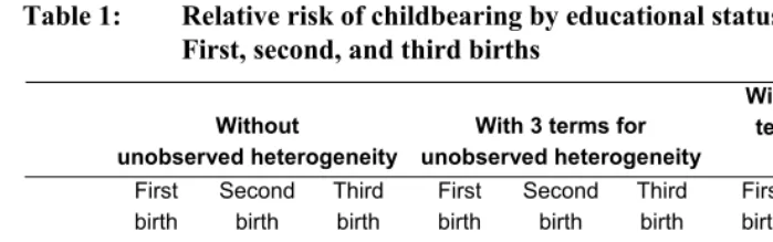
Table 1: Relative risk of childbearing by educational status. First, second, and third births

Without unobserved heterogeneity

With 3 terms for unobserved heterogeneity

With a single common term for unobserved

heterogeneity First birth Second birth Third birth First birth Second birth Third birth First birth Second birth Third birth

Lo ed 1.00 1.00 1.00 1.00 1.00 1.00 1.00 1.00 1.00

Mid ed 0.75 0.75 0.37 0.58 0.74 0.35 0.58 0.57 0.25

Hi ed 0.68 0.65 0.20 0.39 0.62 0.18 0.40 0.37 0.09

In ed 0.28 0.63 0.49 0.19 0.61 0.47 0.20 0.39 0.25

To get this far, we have experimented to some extent with the specification of the distribution of the heterogeneity triple , essentially by working on their correlation matrix. In our preferred specification, we find a notably positive correlation between Ui1and Ui2(we get

1 2 3

{U U Ui, i , i}

12

ˆ

ρ =0.86), and no determinable correlation between U

and the two other heterogeneity factors; in fact, we cannot get convergence of the iterative estimation process that aML uses if we try to introduce a

3

i

13

ρ or a ρ23. The operational consequence is that we take both of these correlations to be zero. Thus, we cannot verify our hypothesis that unobserved characteristics that would make a woman particularly childbearing-prone would manifest themselves across all parities. We are surprised by this finding, and suggest that researchers revisit this feature in future fertility analyses in Romania and other East European countries. At the same time, we note that one of the alternative specifications we have experimented with involves reducing the heterogeneity triple to a single heterogeneity factor U that is common to all three childbearing intensities, which corresponds to setting all correlations '

i

ρllto 1.

The outcome is listed in the final panel of Table 1, the main features of which are the same as in the first two panels; the primary difference is that the educational gradients are even more strongly negative in this final panel.10

Another striking feature of Table 1 is the high fertility of mothers who are currently participating in education, both for the transition to the second and to the third birth (at least in the first two panels of the table). It is as if being in education is not much of an obstacle to further childbearing for women who have already entered

10 _{Many of our predecessors have used a similar one-factor specification. It is possible that a three-factor}

motherhood. We suspect that a finding of this nature may be connected to a weakness in the determination of periods in which a respondent is in education, a weakness that our data share with all data from the first round of the Gender and Generation surveys. It is better to collect proper educational histories than to impute them, as we have been forced to do. We will be able to find out whether such a weakness exists when data from the second wave of GGS surveys become available, as they are designed to focus greater attention on individual educational histories. In the meantime, we offer the following observations about the Romanian educational system that could help to explain why it may indeed be easier than would normally be expected for Romanian women to continue to have children.11

In Romania, mothers enrolled in education most likely are either in a part-time or a distance-learning setting, i.e., they attend high school or vocational training in the evening and/or study through correspondence courses, at weekends, or work toward a tertiary education through distance learning. All of these forms of alternative learning were available to a certain extent in socialist times, and they have become even more widespread in the continuously developing educational environment of democratic Romania.

The socialist regime had the goal of providing working people with access to education, and it organized evening education at the level of vocational and high schools for them. In these schools, the rhythm of teaching was less demanding and the requirements were more relaxed, which was compensated for by a duration of study that was longer than in usual full-time education. Young parents who had been forced to leave daytime school early in order to support their families nonetheless had the opportunity to continue their studies in the evening. While part-time attendance at a university was less available due to a scarcity of openings, access to university did exist in the form of correspondence courses. A recognition of the possibility that opportunities of this kind may have facilitated the combining of enrolment in education and continued childbearing may make the high fertility levels in the last row of Table 1 more plausible.

11 _{Romania may actually share this feature with other countries. In fact, using imputations similar to ours for}

5. Possible explanations for the negative gradients

The negative educational gradient in recent Romanian fertility may be explained by two aspects of the Beckerian theory (in addition to the specific context of Romania). First, more highly educated working mothers may have risked missing wage increases and may have lost skills during maternity leave and childrearing leave. Second, better educated women may have had a stronger preference for higher quality children, rather than for a higher number of children.

Both of these aspects are sides of rational choice theory, but we believe that in Romania the second aspect is the more relevant. More highly educated women probably want to have children who have a high level of human capital, and who are well integrated into the future of a modern society; thus, these mothers are likely to invest much more in their children’s education than are mothers with lower educational levels. (Note that the latter usually live in rural areas or have grown up with “rural” norms and values. In any case, we are unable to control for the character of the current social environment in our data.) The more educated women are more likely to have higher ambitions for their children, and therefore can be expected to devote more energy, time, and money to a smaller number of children.

It is more costly to rear a child adequately for a more highly educated woman, not only because of her higher ambition level, but also because family responsibilities are considered more a duty of the mother than of the father in Romanian society. Even if there is considerable gender equality in the workplace, in families household chores and childrearing are regarded as women’s work.12 _{We extend this theory by arguing that} highly educated and therefore generally more ambitious women are more likely to feel that childrearing is a burden, and that this may lead them to limit their family size to a greater extent than others.

Our findings concerning the fertility effect of educational attainment are based on data for a long period which covers both socialist and post-socialist regimes.13 _The Beckerian “opportunity cost” hypothesis should work well in a society in which wage differentials are large and are connected to educational levels. This was not the case in socialist Romania, where people’s incomes did not differ much according to their educational levels. The introduction of a market economy system led to greater returns on education, and the corresponding considerations related to higher opportunity costs

12 _{Hărăguş (2005) has found evidence of a considerable gender imbalance family work in Romania.}

Incoherence between the levels of gender equity in individually-oriented institutions and family-oriented institutions leaves women facing a difficult choice between work and family, and MacDonald (2000) has argued that low fertility is correlated with the degree of such incoherence.

13 _{Given this perspective, educational effects may actually have changed over time, but we have not wanted to}

led to a lowering of the birth risk among more educated women, as we indicated at the beginning of this paper.

When even more highly educated women have their first child early, they have little reason to feel any time squeeze in their progression to subsequent births, and are likely to have children at a rather leisurely pace. This feature may in itself produce rates of second and third births that are lower for the more highly educated, which will be reflected in negative educational gradients of childbearing similar to those identified in our intensity regressions.14

6. Acknowledgements

We are grateful for constructive comments from two reviewers and from the main editor of the present journal.

References

Becker, G. (1981). A Treatise on the Family. Cambridge: Harvard University Press. Gjonca, A., Aassve, A., and Mencarini, L. (2008). Albania: Trends and patterns,

proximate determinants and policies of fertility change. Demographic Research 19(11): 261-292. doi:10.4054/DemRes.2008.19.11.

Hărăguş, P.-T. (2005). Folosirea timpului şi sarcinile domestice în Europa (Time use and domestic work in Europe). Studia Universitatis Babeş-Bolyai Sociologia 2: 95-116.

Hoem, B. (1996). The social meaning of the age at second birth for third-birth fertility: A methodological note on the need to sometimes re-specify an intermediate variable. Yearbook of Population Research in Finland 33: 333-339.

Hoem, J.M., Prskawetz, A., and Neyer, G.R. (2001). Autonomy or conservative adjustment? The effect of public policies and educational attainment on third births in Austria, 1975-96. Population Studies 55(3): 249-261.

doi:10.1080/00324720127700.

Hoem, J.M. and Kreyenfeld, M. (2006). Anticipatory analysis and its alternatives in life-course research. Part 1: The role of education in the study of first childbearing. Demographic Research 15(16): 461-484. doi:10.4054/DemRes. 2006.15.16.

Köppen, K. (2006). Second births in Western Germany and France. Demographic Research 14(14): 295-330. doi:10.4054/DemRes.2006.14.14.

Koytcheva, E. (2006). Social-demographic differences of fertility and union formation in Bulgaria before and after the start of the societal transition. [PhD

dissertation] University of Rostock, Available from the Max Planck Institute for Demographic Research.

Kravdal, Ø. (2001). The high fertility of college educated women in Norway: An artefact of separate modelling of each parity transition. Demographic Research 5(6): 185-215. doi:10.4054/DemRes.2001.5.6.

Kravdal, Ø. (2004). An illustration of the problems caused by incomplete education histories in fertility analyses. Demographic Research SC3(6): 135-154.

Kreyenfeld, M. (2002). Time-squeeze, partner effect or self-selection? An investigation into the positive effect of women's education on second birth risks in West Germany. Demographic Research 7(2): 15-47. doi:10.4054/DemRes.2002.7.2. Kreyenfeld, M. and Zabel, C. (2005). Female education and the second child: Great

Britain and Western Germany compared. Zeitschrift für Wirtschafts- und Sozialwissenschaften/Schmollers Jahrbuch 125: 145-156.

McDonald, P. (2000). Gender equity, social institutions and the future of fertility. Journal of Population Research 17(1): 1-16. doi:10.1007/BF03029445.

Mureşan, C. (1996). L'évolution démographique en Roumanie: Tendances passées (1948-1994) et perspectives d'avenir (1995-2030). Population 51(4/5): 813-844. Mureşan, C. (2008). Impact of induced abortion on fertility in Romania. European

Journal of Population 24(4): 425-446. doi:10.1007/s10680-008-9151-0.

Mureşan, C., Hărăguş, P.-T., Hărăguş, M., and Schröder, C. (2008). Overview Chapter 6: Romania: Childbearing metamorphosis within a changing context. Demographic Research 19(23): 855-906. doi:10.4054/DemRes.2008.19.23. Oláh, L. (2003). Gendering fertility: second births in Sweden and Hungary. Population

Research and Policy Review 22(2): 171-200. doi:10.1023/A:1025089031871. Perelli-Harris, B. (2008). Ukraine: On the border between old and new in uncertain

times. Demographic Research 19(29): 1145-1178. doi:10.4054/DemRes. 2008.19.29.

Appendix 1: Construction of the variable “current educational

attainment” and considerations concerning exposure time

Given the lack of complete educational histories, we have imputed a current educational level from our GGS data, first by separating for each individual the time spent in education from the time after education has been completed, and then by identifying those who have finished education by educational level attained. Only women who had completed at least lower-secondary education (which is compulsory in Romania) reported the date they achieved it, so for women without education or with primary education only, we have had to impute the date they finished their education. We set this date as the respondent’s 12th _{birthday, which we take to be the age when a woman} becomes exposed to the risk of giving birth. Every respondent is considered to be enrolled in full-time education until the date of her declared completion of final education. Such a definition of educational enrolment is strongly anticipatory, i.e., it assumes that the respondent did not take breaks between completing different educational levels. Until the late 1990s, when alternatives to daytime higher education started to emerge with some regularity, there were limited opportunities for returning to the educational system, and thus we can have confidence in our imputation for such periods. By contrast, strong anticipatory bias could affect our findings post 2000, since more students, especially women, and including mothers, returned to the educational system to earn a first degree diploma, which is required by the new professions of the market economy. Without making further assumptions, we cannot distinguish between women currently enrolled in high school, vocational school, or undergraduate studies. Those who were participating in education at the time of interview are considered to be enrolled full time. After completion, we have assigned the reported educational level to the respondent.

For the sake of simplicity, we have grouped the educational levels into just three categories, low, medium, and high, as follows:

• “Low level of education” means no academic qualifications. Respondents who did not report that they had graduated from high school, but who had attended primary school, middle school, and high school (first cycle only, giving a maximum of 10 grades, ISCED Levels 0, 1, and 2) are in this category. They have no more than compulsory education.

• “High level of education” means at least a university degree. All holders of an academic degree are in this category, as are graduates of short-cycle and long-cycle university programs, and of more advanced tertiary education (ISCED Levels 5 and 6).

In total we have four educational statuses, three of them categorized as with a completed education, and one additional category which amalgamates the statuses of being currently enrolled regardless of the level of education. We operate with no transitions between educational levels, except from the status “in education” into a “low,” “medium” or “high” educational level. Transition to motherhood or to a higher parity is possible from each of the four educational statuses without any change in the educational level.

Appendix 2: Other features of our period analysis

a) Baseline intensities for first, second, and third births

Figure 2A: First-birth baseline, by age of mother

0 50 100 150 200 250 300

15 20 25 30 35 40

age of women

h

azar

d

p

er

1

000

p

er

so

n

-year

s Separate Models

Joint Model

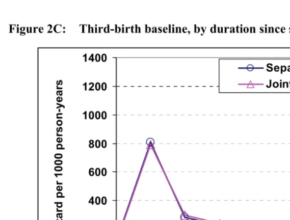
Figure 2B: Second-birth baseline, by duration since first birth

0 100 200 300 400 500 600

0 2 4 6 8 10 12 14

age of first child

h

az

ar

d

p

er

100

0 p

er

so

n

-y

ear

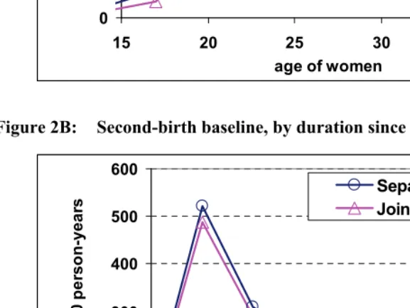
Figure 2C: Third-birth baseline, by duration since second birth

0 200 400 600 800 1000 1200 1400

0 2 4 6 8 10 12 14

age of second child

ha

za

rd p

e

r 1

0

0

0

pe

rs

on-y

e

a

rs

Separate Models Joint Model

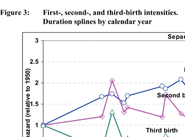
b) Period effects

Figure 3 contains the period effects for each birth order. For second and third births, we see clear effects of the variations in public family policy, and in all curves we see a general effect of institutional and economic changes, in particular the fertility decline after the end of communism, as described above at the end of Chapter 3. The prohibition of abortion in 1967 appears as a clear jump in the period curves for second and third births in that year. We are surprised that there is almost no corresponding jump in the curve for first births. As Mureşan (2008) has shown based on other data, this suggests that women did not use abortion as a means of fertility control before their first birth nearly as extensively as women who had already entered motherhood.

Figure 3: First-, second-, and third-birth intensities. Duration splines by calendar year

0 0.5 1 1.5 2 2.5 3

1950 1960 1970 1980 1990 2000

h

az

ar

d

(r

el

ati

ve t

o

19

50

) _{First birth}

Second birth

Third birth

Separate Models

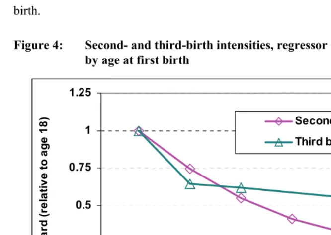
c) The effect of age at first birth on the intensities of second and third birth

The impact of age at first birth on second- and third-birth risks appears in Figure 4. The figure shows that the second- and third-birth intensities decline uniformly as the age at first birth increases. These curves come from our models without heterogeneity elements. The corresponding curves from models with heterogeneity factors are not much different, and are not displayed here. We believe, however, that the models we have used up to this point are too simple to pick up subtler effects of age at first births on later fertility. For example, entering motherhood at age 22 must have a different social meaning15 _{for women with higher levels of education (few of whom become} mothers at such a tender age) than it has for women with very little education (most of whom actually have their first child before age 22). Conversely, very few women with little education have a first child in their late twenties, while this is quite a normal age for entering motherhood among the more highly educated. We plan to pay attention to

the interaction between educational attainment and age at first birth in future work on second- and third-birth risks. We expect unobserved heterogeneity to play a more prominent role in that analysis than it has in the present paper because educational differentials in attitudes and values would no doubt be reflected in different ages at first birth.

Figure 4: Second- and third-birth intensities, regressor splines

by age at first birth

0 0.25 0.5 0.75 1 1.25

15 20 25 30 35

age at first birth

h

az

a

rd

(

re

la

ti

v

e t

o

ag

e 18

)

40 Second birth

Third birth