A shifted Chebyshev-Tau method for finding a time-dependent heat
source in heat equation
Samaneh Akbarpour
Department of Mathematics, Lahijan Branch, Islamic Azad University, Lahijan, Iran. E-mail: [email protected]
Abdollah Shidfar
Department of Mathematics, Lahijan Branch, Islamic Azad University, Lahijan, Iran. E-mail: [email protected]
Hashem Saberi Najafi∗
Department of Mathematics, Lahijan Branch, Islamic Azad University, Lahijan, Iran. E-mail: [email protected]
Abstract This paper investigates the inverse problem of determining the time-dependent heat source and the temperature for the heat equation with Dirichlet boundary conditions and an integral over-determination conditions. The numerical method is presented for solving the Inverse problem. Shifted Chebyshev polynomial is used to approxi-mate the solution of the equation as a base of the tau method which is based on the Chebyshev operational matrices. The main advantage of this method is based upon reducing the partial differential equation into a system of algebraic equations of the solution. Numerical results are presented and discussed.
Keywords. Inverse source problem, Heat equation, Shifted Chebyshev polynomial, Operational matrix,
Shifted Chebyshev-Tau method .
2010 Mathematics Subject Classification. 35R30, 65N21, 58J35.
1. Introduction
The inverse problems for heat equation arise in many physical and engineering problems, and they can be roughly divided into three principal classes.
(1) Backward or reversed-time problem: the initial condition is to be found [16, 26].
(2) Coefficient inverse problem: this is a classical parameter problem where a multiplier in the governing equation is to be found [1,5,8,11,17,22,24,25, 27].
(3) Boundary inverse problem: some missing information at the boundary of the domain is to be found [10, 18, 19,23].
Received: 20 April 2018 ; Accepted: 9 December 2018.
∗Corresponding author.
In this paper, we consider the following heat equation:
ut(x, t) =uxx(x, t) +p(t)u(x, t) +q(x, t), 0< x < L, 0< t≤τ, (1.1)
with initial condition
u(x,0) =f(x), 0< x < L, (1.2)
and the Dirichlet boundary conditions
u(0, t) =g1(t), 0< t≤τ, (1.3)
u(L, t) =g2(t), 0< t≤τ, (1.4)
subject to the integral over-specification of the functionk(x)u(x, t) over the spatial domain (energy over-specification)
Z 1
0
k(x)u(x, t)dx=E(t), 0≤t≤τ (1.5)
whereq(x, t), f(x), g1(t), g2(t), k(x), E(t)6= 0 are given functions. Also, it is
as-sumed that for constantρ >0 the kernel k(x) satisfies
Z 1
0
|k(x)|dx≤ρ.
If the functionp(t) is known, the problem of findingu(x, t) from (1.1)-(1.4) is called the direct problem. However, the problem here is that the source parameter p(t) is unknown, which needs to be determined by energy condition (1.5). This problem (1.1)–(1.5) is called the inverse problem.
There is a fundamental difference between the direct and inverse problems. It is known that an inverse problem is not well posed in general while the direct problem is well posed. The existence and uniqueness of this inverse problem are discussed in [4, 6, 13, 15, 17, 20]. In [6, 7, 11, 17, 21] the solution of this problem and similar problems are investigated. Some numerical methods are presented in [11, 17] for solving this problem. In [17], the author used the high order scheme for the solution of inverse problem (1.1)–(1.5). Also, the numerical methods suggested in [11] are based on the optimal homotopy analysis method (OHAM) is designed.
2. Properties of shifted Chebyshev polynomials
The well-known shifted Chebyshev polynomials are defined on the interval [0,1] and can be determined with the aid of the following recurrence formulae:
TL,0(x) = 1, TL,1(x) =
2x L −1,
TL,j(x) = 2
2x
L −1
TL,j−1(x)−TL,j−2(x), j= 2,3, ..., n. (2.1)
The following formula for thejth degree ofTL,j(x)
TL,j(x) =j j
X
k=0
(−1)j−k (j+k−1)!2
2k
(j−k)! (2k)!Lkx
k, j= 1,2,3, ..., n, (2.2)
whereTL,j(0) = (−1) j
andTL,j(L) = 1. The orthogonality condition is
Z L
0
TL,j(x)TL,k(x)wL(x)dx=hj, (2.3)
where
wL(x) = 1 √
Lx−x2, (2.4)
and
hj =
εj
2π , k=j,
0 , k6=j,
ε0= 2, εj= 1; j≥1. (2.5)
A functionu(x, t) of two independent variables defined for 0< x < L,0< t≤τ may be expanded into the shifted Chebyshev polynomials as:
u(x, t) =
∞ X
i=0 ∞ X
j=0
aijTτ,i(t)TL,j(x). (2.6)
If the infinite series in (2.6) is truncated, then it can be written as:
um,n(x, t)' m
X
i=0
n
X
j=0
aijTτ,i(t)TL,j(x) =ψT(t)Aφ(x), (2.7)
where the shifted Chebyshev vectorsψ(t) andφ(x) and the shifted Chebyshev coef-ficient matrixAare given as:
ψ(t) = [Tτ,0(t), Tτ,1(t), ..., Tτ,m(t)]T,
φ(x) = [TL,0(x), TL,1(x), ..., TL,n(x)] T
, (2.8)
A=
a00 a01 · · · a0n a10 a11 · · · a1n
..
. ... · · · ... am0 am1 · · · amn
where
aij = 1 hihj
Z τ
0 Z L
0
u(x, t)Tτ,i(t)TL,j(x)wτ(t)wL(x)dxdt, (2.9)
i= 0,1, ..., m, j= 0,1, ..., n.
Theorem 2.1. The first derivative of the shifted Chebyshev vector φ(x) may be expressed by[2,3, 9,14]
dφ(x) dx =D
(1)φ(x), (2.10)
whereD(1) is the(n+ 1)×(n+ 1)operational matrix of derivative given by
D(1) =dij =
4i
εjL j=i−k,
k= 1,3, ..., n
k= 1,3, ..., n−1
if (n) is odd
if (n)is even 0 otherwise
(2.11)
whereε0= 2, εj= 1, j≥1 .
For example, for odd n given as:
D= 2 L
0 0 0 · · · 0 0 0
1 0 0 · · · 0 0 0
0 4 0 · · · 0 0 0
3 0 6 · · · 0 0 0
..
. ... ... . .. ... ... ... 0 2 (n−1) 0 · · · 2 (n−1) 0 0
n 0 2n · · · 0 2n 0
and for even n given as:
D= 2 L
0 0 0 · · · 0 0 0
1 0 0 · · · 0 0 0
0 4 0 · · · 0 0 0
3 0 6 · · · 0 0 0
..
. ... ... . .. ... ... ... n−1 0 2 (n−1) · · · 2 (n−1) 0 0
0 2n 0 · · · 0 2n 0
Remark 2.2. The operational matrix for the nth derivative can be derived as [7,9]
dnφ(x) dxn =
D(1) n
φ(x), (2.12)
wheren∈N and the superscript inD(1) , denotes matrix powers. Thus
Dn =D(1) n
Theorem 2.3. The integration ofψτ,m(t) may be written as [23, 25]
Z t
0
ψ(t0)dt0'P ψ(t), (2.14)
whereP is the (m+ 1)×(m+ 1)shifted Chebyshev operational matrix of integration and is given by
p=
w0 δ0 0 0 0 · · · 0 0
w1 0 λ1 0 0 · · · 0 0
w2 δ2 0 λ2 0 · · · 0 0
w3 0 δ3 0 λ3 · · · 0 0 ..
. ... ... . .. . .. . .. ... ...
wm−2 0 0 0 . .. . .. λm−2 0
wm−1 0 0 0 0 . .. 0 λm−1
wm 0 0 0 0 · · · δm 0
, (2.15) where
wk =
τ
2 , k= 0
−τ
8 , k= 1
(−1)k+1τ
2(k−1)(k+1) , k= 2,3, ...
, δk=
τ
2 , k= 0
0 , k= 1
−τ
4(k−1) , k= 2,3, ...
,
λk =
0 , k= 0
τ
8 , k= 1
τ
4(k+1) , k= 2,3, ...
(2.16)
Obviously similar to (2.14) we have
Z x
0
φ(x0)dx0'Gφ(x), (2.17)
whereG is the (n+ 1)×(n+ 1) shifted Chebyshev operational matrix of integration and is defined similar to (2.15).
3. The numerical scheme
as:
um,n(x, t) =ψT(t)Aφ(x), (3.1)
qm,n(x, t)' m X i=0 n X j=0
qijTτ,i(t)TL,j(x) =ψT(t)Qφ(x),
f(x)' n
X
j=0
fjTL,j(x) =ψT(t)F φ(x),
whereAis an unknown (m+ 1)×(n+ 1) matrix,QandFare known (m+ 1)×(n+ 1) matrices, as Q=
q00 q01 · · · q0n q01 q11 · · · q1n
..
. ... ... ... qm0 qm1 · · · qmn
, F =
f0 f1 · · · fn−1 fn 0 0 · · · 0 0
..
. ... · · · ... ... 0 0 · · · 0 0
, (3.2) where
qij = 1 hihj
Z τ
0 Z L
0
q(x, t)Tτ,i(t)TL,j(x)wτ(t)wL(x)dxdt, (3.3)
i= 0,1, ..., m, j= 0,1, ..., n
and
fj= 1 hj
Z L
0
f(x)TL,j(x)wL(x)dx, j= 0,1, ..., n. (3.4)
Integrating equation (1.1) from 0 totand using equation (1.2) (see [7,9]), we have
u(x, t)−f(x) =
Z t
o
uxx(x, t0)dt0+
Z t
o
p(t0)u(x, t0)dt0+
Z t
o
q(x, t0)dt0. (3.5)
Using equations (2.7), (2.12) and (2.14) we get
Z t
o
uxx(x, t0)dt0=
Z t
o
ψT(t0)dt0
A
d2φ(x)
dx2
=ψT(t)PTAD2φ(x). (3.6)
The functionp(t) may be expanded in terms ofm+ 1 shifted Chebyshev series as
p(t) = m
X
k=0
bkTτ,k(t) =BTψ(t), (3.7)
whereB= [b0, b1, ..., bm] T
is an unknown vector. Now, using equations (2.5), (2.12) and (3.7) we have
Z t
o
p(t0)u(x, t0)dt0=
Z t
o
BTψ(t0)ψT(t0)dt0
Aφ(x). (3.8)
Let
whereH is an (m+ 1)×(m+ 1) matrix. To findH, we rewrite equation (3.9) (see[23]) in the form
m
X
k=0
bkTτ,k(t)Tτ,j(t) = m
X
k=0
HkjTτ,k(t), j= 0,1, ..., m. (3.10)
Multiplying the both sides of (3.10) byTτ,i(t)wτ(t) ,i= 0,1, ..., mand integrating from 0 toτ yield
m
X
k=0
bk
Z τ
0
Tτ,i(t)Tτ,k(t)Tτ,j(t)wτ(t)dt
= m
X
k=0
Hkj
Z τ
0
Tτ,k(t)Tτ,i(t)wτ(t)dt, i, j= 0,1, ..., m. (3.11)
Using equation (3.11) and employing the orthogonality relation (2.3) give
m
X
k=0
bk
Z τ
0
Tτ,i(t)Tτ,k(t)Tτ,j(t)wτ(t)dt=Hijhi,
or equivalently
Hij = 1 hi
m
X
k=0
bk
Z τ
0
Tτ,i(t)Tτ,k(t)Tτ,j(t)wτ(t)dt, i, j= 0,1, ..., m. (3.12)
Employing equations (2.14), (3.8) and equation (3.9) can be written as
Z t
o
p(t0)u(x, t0)dt0=ψT(t)PTHAφ(x). (3.13)
Also by using equations (2.7), (2.14) and (3.1) (see [23]), we get
Z t
o
q(x, t0)dt0=
Z t
0
ψT(t0)dt0
Qφ(x) =ψT(t)PTQφ(x). (3.14)
Applying equations (2.7), (3.1), (3.6), (3.13) and (3.14) the residual Rm,n(x, t) for equation (3.5) can be written as
Rm,n(x, t) =ψT(t)A−F−PTHA−PTAD2−PTQφ(x) = 0.
Let
Z=
A−F−PTHA−PTAD2−PTQ
,
then we have
ψT(t)Zφ(x) = 0. (3.15)
As in a typical Tau method, we generate (m+ 1)×(n−1) linear algebraic equations using the following algebraic equations
Also, by substituting equations (3.1) and (3.7) in equations (1.3)-(1.4) we get
ψT(t)Aφ(0) =g1(t), (3.17)
ψT(t)Aφ(L) =g2(t). (3.18)
And applying (3.1) in equation (1.5), we have
Z 1
0
k(x)u(x, t)dx=ψT(t)A
Z 1
0
k(x)φ(x)dx
=E(t). (3.19)
Let’s assume that
I=
Z 1
0
k(x)φ(x)dx, (3.20)
and
I= [I0, I1, I2, ..., In] T
, i= 0,1,2, ..., n (3.21)
with
Ii=
Z 1
0
k(x)φi(x)dx, (3.22)
that
k(x)' n
X
j=0
kjTL,j(x) =ψT(t)Kφ(x), (3.23)
andKis known (m+ 1)×(n+ 1) matrix below
K=
k0 k1 · · · kn−1 kn 0 0 · · · 0 0
..
. ... · · · ... ... 0 0 · · · 0 0
,
that is
kj = 1 hj
Z L
0
k(x)TL,j(x)wL(x)dx. (3.24)
Now applying equations (3.20)-(3.24) in equation (3.19), we have
ψT(t)AI=E(t). (3.25)
Figure 1. Plot of error for|um,n(x,1)−u(x,1)|withm=n= 4,8.
Figure 2. Plot of error for|pm(t)−p(t)|withm=n= 2,8.
4. Numerical results
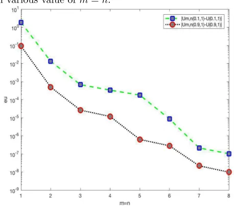
Figure 3. Plot of error |um,n(x,1)−u(x,1)| forx= 0.1 and x= 0.9 with various value ofm=n.
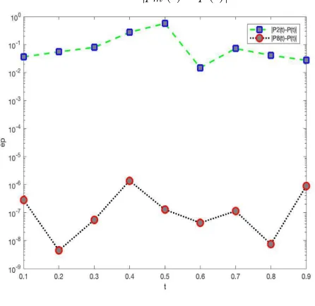
Figure 4. Plot of error|pm(t)−p(t)| fort= 0.1 andt= 0.9 with various value ofm.
shifted chebyshev-Tau method based on absolute errorseu andep defined as:
eu=|um,n(x, t)−u(x, t)|, ep=|pm(t)−p(t)|
Example 4.1. The inverse problem (1.1)–(1.5) with the following conditions:
τ= 1, L= 1,
q(x, t) = exp (t) x+cos(πx) +π2cos(πx)−exp (t) 1 +t2(x+cos(πx)), f(x) =x+cos(πx),
g1(t) = exp (t),
g2(t) = 0,
E(t) = exp 34− 2
π2
, k(x) = 1 +x2
The exact solution of the problem isu(x, t) = exp (t) (x+ cosπx) andp(t) = 1 +t2, see [17,11].
We solved the problem by applying the method described in Section 3. We re-port the absolute error of |um,n(x,1)−u(x,1)| and |pm(t)−p(t)| for m = n = 4,6,8 in Tables 1 and 2, respectively. Figure 1 shows the absolute error function |um,n(x,1)−u(x,1)| at different space for m = n = 4,8 . In addition, Figure 2 shows the absolute error function|pm(t)−p(t)|at different time for m =n= 2,8. Also, Figure 3 and Figure 4 illustrate the numerical results of the error function |um,n(x,1)−u(x,1)|and|pm(t)−p(t)|by increasing ofmandnin 0.1 and 0.9.
The obtained results showed that this approach can solve the problem effectively. The described computational method produces very accurate results even when em-ploying a small number of collocation points.
Table 1. Results for u(x,1) and the absolute error |um,n(x,1)−u(x,1)|form Example.
x exact error
u(x,1) m=n= 4 m=n= 6 m=n= 8 0.1 2.8571e+00 3.3395e-04 8.5616e-06 1.0265e-07 0.2 2.7428e+00 2.1271e-04 3.3107e-08 1.1036e-09 0.3 2.4133e+00 1.4184e-04 1.7740e-06 7.0921e-09 0.4 1.9273e+00 1.6643e-04 3.7018e-06 4.4484e-08 0.5 1.3591e+00 2.4769e-04 1.7070e-05 2.8897e-06 0.6 7.9097e-01 1.4388e-05 2.4996e-07 2.2013e-09 0.7 3.0503e-01 2.2960e-05 2.4139e-07 2.6079e-09 0.8 -2.4511e-02 1.8292e-07 5.9385e-10 1.8227e-11 0.9 -1.3879e-01 1.1727e-05 2.8145e-07 9.8509e-09
5. Conclusion
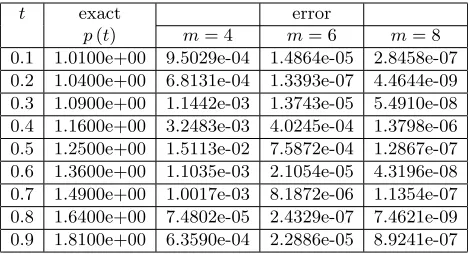
Table 2. Results forp(t) and absolute error|pm(t)−p(t)| form Example.
t exact error
p(t) m= 4 m= 6 m= 8
0.1 1.0100e+00 9.5029e-04 1.4864e-05 2.8458e-07 0.2 1.0400e+00 6.8131e-04 1.3393e-07 4.4644e-09 0.3 1.0900e+00 1.1442e-03 1.3743e-05 5.4910e-08 0.4 1.1600e+00 3.2483e-03 4.0245e-04 1.3798e-06 0.5 1.2500e+00 1.5113e-02 7.5872e-04 1.2867e-07 0.6 1.3600e+00 1.1035e-03 2.1054e-05 4.3196e-08 0.7 1.4900e+00 1.0017e-03 8.1872e-06 1.1354e-07 0.8 1.6400e+00 7.4802e-05 2.4329e-07 7.4621e-09 0.9 1.8100e+00 6.3590e-04 2.2886e-05 8.9241e-07
Illustrative numerical example with satisfactory approximate solutions is achieved to demonstrate the accuracy of method. The numerical results in Section 4 demonstrate the good accuracy of the described method. Moreover, only a small number of shifted Chebyshev polynomials is needed to obtain a satisfactory solution.
References
[1] S. Akbarpour, A. Shidfar, and H. Saberi Najafi,Shifted Chebyshev-Tau method for solving an inverse time-dependent source problem, Applied Mathematical and Computational Sciences,9 (2017), 1–20.
[2] M. H. Atabakzadeh, M. H. Akrami, and G. H. Erjaee,Chebyshev operational matrix method for solving multi-order fractional ordinary differential equations, Applied Mathematical Modelling, 37(2013), 8903–8911.
[3] C. Canuto, M. Y. Hussaini, A. Quarteroni, and T. A. Zang,Spectral Methods in Fluid Dynamic, Prentice-Hall, Englewood Cliffs, NJ, 1988.
[4] J. R. Cannon and Y. Lin, An inverse problem of ?nding a parameter in a semilinear heat equation, J. Math. Anal. Appl,145(1990), 470–484.
[5] Q. Chen and J. Liu,Solving an inverse parabolic problem by optimization from ?nal measure-ment data, J. Comput. Appl. Math,193(2006), 183–203.
[6] M. Dehghan,Parameter determination in a partial differential equation the overspeci?ed data, Math. Comput. Model,41(2005), 197–213.
[7] M. Dehghan and A. Saadatmandi, and A. Compo,The Legender-Tau technique for the deter-mination of a source parameter in a semilinere parabolic equation, Mathematics problems in engineering,2006(2006), 1-11.
[8] M. Dehghan and M. Tatari,Solution of a semilinear parabolic equation with an unknown control function using the decomposition procedure of Adomian, Numer. Methods Partial Differ. Equ, 23(2007), 499–510.
[9] E. H. Doha, A. H. Bhrawy, and S. S. Ezz-Eldien, Numerical approximations for fractional diffusion equations via a chebyshev spectral-tau method, Cent.Eur.J.phys,11(2013), 1494-1503. [10] Y. C. Hon and M. Li,A computational method for inverse free boundary determination problem,
Int. J. Numer. Methods Eng,73(2008), 1291–1309.
[11] A. Jaradat, F. Awawdeh, and M. S. M. Noorani,Identification of time-dependent source terms and control parameters in parabolic equations from overspecified boundary data, Journal of Computational and Applied Mathematics,313(2016), 397–409.
[13] Y. Lin,Analytical and numerical solutions for a class of nonlocal nonlinear parabolic differential equations, SIAM J. Math. Anal,25(1994), 1577–1594.
[14] Y. Luke,The Special Functions and Their Approximations, vol. 2, Academic Press, New York, 1969.
[15] J. A. Macbain and J. B. Bendar, Existence and uniqueness properties for one-dimensional magnetotelluric inversion problem, J. Math. Phys,27(1986), 645–649.
[16] N. S. Mera, L. Elliott, D. B. Ingham, and D. Lesnic,An iterative boundary element for solving the one-dimensional backward heat conduction problem, Int. J. Heat Mass Transfer,44(2001) 1937–1946.
[17] A. Mohebbi and M. Dehghan, High-order scheme for determination of a control parameter in an inverse problem from the over-specified data, Computer Physics Communications, 181 (2010), 1947–1954.
[18] T. T. M. Onyango, D. B. Ingham, and D. Lesnic,Restoring boundary conditions in heat con-duction, J. Eng. Math,62(2008), 85–101.
[19] T. T. M. Onyango, D. B. Ingham, D. Lesnic, and M. Slodicka,Determination of a time de-pendent heat transfer coefficient from non-standard boundary measurements, Math. Comput. Simul,79(2009), 1577–1584.
[20] A. I. Prilepko and V. V. Soloev,Solvability of the inverse boundary value problem of finding a coefficient of a lower order term in a parabolic equation, Differential Equations,23 (1987), 136–143.
[21] W. Rundell,Determination of an unknown non-homogeneous term in a linear partial differen-tial equation from overspeci?ed boundary data, Appl. Anal,10(1980), 231–242.
[22] A. Shidfar and R. Zolfaghari,Restoration of the hat transfer coefficient from boundary mea-surements using the sinc method, comp.Appl.Math,3(2015), 29–44.
[23] A. Shidfar and R. Zolfaghari,Reconstructing an unknown time-dependent function in the bound-ary condition of a parabolic PDE, Journal of Applied Mathematics and computation,225(2014), 238–249.
[24] A. Shidfar and R. Zolfaghari,Determination of an unknown function in a parabolic inverse problem by Sinc-collocation method, Numer. Methods Partial Differ. Equ,27(2011), 1584–1598. [25] A. Shidfar, R. Zolfaghari, and J. Damirchi,Appliation of sinc-colloation method for solving an
invrse problem, Jornal of computational and Applied Mathematics,233(2009), 545–554. [26] M. Tadi,An iterative method for the solution of ill-posed parabolic systems, Appl. Math.
Com-put,201(2008), 843–851.