An application of differential transform method for solving
nonlin-ear optimal control problems
Alireza Nazemi∗ Department of Mathematics, School of Mathematical Sciences, Shahrood University of Technology,
P.O. Box 3619995161-316, Tel-Fax No:+98 23-32300235, Shahrood, Iran.
E-mail: [email protected]
Saiedeh Hesam
Department of Mathematics, School of Mathematical Sciences, Shahrood University of Technology,
P.O. Box 3619995161-316, Tel-Fax No:+98 23-32300235, Shahrood, Iran.
E-mail: [email protected]
Ahmad Haghbin
Department of Mathematics, Gorgan branch, Islamic Azad University, Gorgan, Iran. E-mail: [email protected]
Abstract In this paper, we present a capable algorithm for solving a class of nonlinear optimal control problems (OCP’s). The approach rest mainly on the differential transform method (DTM) which is one of the approximate methods. The DTM is a powerful and efficient technique for finding solutions of nonlinear equations without the need of a linearization process. Utilizing this approach, the optimal control and the corresponding trajectory of the OCP’s are found in the form of rapidly convergent series with easily computed components. Numerical results are also given for several test examples to demonstrate the applicability and the efficiency of the method.
Keywords. Optimal control problems; Differential transform method; Hamiltonian system. 2010 Mathematics Subject Classification. 49J15.
1. Introduction
Optimal control problems arise in a wide variety of scientific and engineering ap-plications including physics, aerospace engineering, robotics, chemical engineering, economy, etc. [14,28,30,34]. In practice, many optimal control problems are sub-ject to constraints on the state and/or control variables. It is well known that con-strained optimal control problems are very difficult to solve. In particular, their analytical solutions are in many cases out of the question. Thus, numerical meth-ods are needed for solving many of these real world problems. There are now many
Received: 19 February 2016 ; Accepted: 25 July 2016.
∗Corresponding author.
numerical methods available in the literature for various optimal control problems [1,3,6,8,9,11,15,21–24,26,31–33,36]. Among them, Bellman [7] proposed an approach using dynamic programming. This approach leads to the Hamilton- Jacobi-Bellman (HJB) equation which is hard to solve in most cases. Due to the use of embedding method, Rubio [32] proposed a numerical approach for solving optimal control prob-lems of ODE’s and PDE’s. The advantages of the proposed method lies on the fact that the method is not iterative, it is self-starting, and it does not need to solve corresponding boundary value problems. However, this method has high computa-tional complexity. Huang and Lin [21] and Abu-khalaf et al. [1] suggested a numerical approach which finds the Taylor series solution of the Hamilton-Jacobi-Isaacs (HJI) equation associated with the nonlinearH∞ control problem. The coefficients of the Taylor series are generated by solving one Riccati algebraic equation and a sequence of linear algebraic equations. However, deriving each linear equation in the sequence requires a number of matrix computations, which may introduce computational com-plexity. An excellent literature review on the methods for solving the HJB equation is provided by Beard et al. [6] where a Successive Galerkin Approximation (SGA) approach is also considered. In the SGA, a sequence of generalized HJB equations is solved iteratively to obtain a sequence of approximations leading eventually to the solution of the HJB equation. However, the above-mentioned sequence may converge very slowly or even diverge. Banks and Dinesh [4] proposed the Approximating Se-quence of Riccati Equations (ASRE). From a practical point of view, the ASRE is attractive. But its shortcoming is that it suffers from computational complexity, since it needs solving a sequence of linear quadratic time-varying matrix Riccati differen-tial equations. Cimen [9] presented the State-Dependent Riccati Equation (SDRE) method which has been widely used in various applications. However, its major lim-itation is that it requires solving a sequence of matrix Riccati algebraic equations. This property may use up a lot of computing time and memory space.
One well known method for solving optimal control problems can also be derived using the Pontryagin’s maximum principle (PMP) [31]. For the nonlinear OCP’s, this approach leads to a nonlinear Two-Point Boundary Value Problem (2PBVP) that unfortunately in general cannot be analytically solved. Therefore, many re-searchers have tried to find an approximate solution for the nonlinear 2PBVPs [3]. In the recent years, some better results have been obtained. For instance, a new Suc-cessive Approximation Approach (SAA) has been proposed by Tang in [33], where instead of directly solving the nonlinear 2PBVP, derived from the maximum princi-ple, a sequence of nonhomogeneous linear time-varying 2PBVPs is solved iteratively. It should be noted that solving time-varying equations are much more difficult than solving time-invariant ones. Effati and Saberi Nik [11] obtained an analytical approx-imate solution for non-linear OCP’s using the homotopy perturbation method. As a modification, Jajarmi et al. [23] applied the optimal homotopy perturbation method for OCP’s. Yousefi et al. [36] utilized another approximate analytical scheme called the variational iteration method to find optimal control of linear systems.
initial value problems in electric circuit analysis. This method constructs an analytical solution in the form of polynomials. It is different from the high-order Taylor series method, which requires symbolic computation of the necessary derivatives of the data functions. The Taylor series method is computationally expansive for large orders. The differential transform is an iterative procedure for obtaining analytic Taylor series solutions of differential equations. In recent years the application of differential transform theory has been appeared in many researches [2,10,12,17,19, 20,25,27,35,37]. Especially, the differential transform method has been successfully used for solving 2PBVP [5,13,18,29].
Motivated by the above discussions, the aim of this paper is to employ the DTM for solving a class of linear and nonlinear OCP’s. Applying the DTM to the 2PBVP derived from the PMP, the optimal control and the corresponding trajectory are obtained in the form of rapid convergent series. Moreover, the convergence of the obtained series is controlled by an absolute tolerance. Thus, just a few iterations yield to find a suboptimal trajectory-control pair for the nonlinear OCP’s. Illustrative examples are provided to demonstrate the applicability and efficiency of the technique. The paper is organized as follows. Section 2 describes the mathematical modelling of a linear-quadratic OCP’s which using PMP leads to a linear 2PBVP. Section 3 is similar to section 2, where instead of linear-quadratic OCP’s, a nonlinear OCP’s with the corresponding 2PBVP is studied. The basic idea of DTM is explained in Section 4. In Section 5, the DTM is employed to propose a new optimal control design strategy. In Section 6, effectiveness of the proposed approach is verified by solving several numerical examples. Conclusions are given in Section 7.
2. Linear-quadratic optimal control system Consider the linear system
˙
x=Ax(t) +Bu(t), t0≤t≤tf, (2.1)
with the initial condition
x(t0) =x0, (2.2)
where x0 ∈ Rn is a given vector and the matrices A ∈ Rn×n and B ∈ Rm×n. we
shall consideru∈Lm
2 [t0, tf] andx: [t0, tf] →Rn an absolutely continuous function on [t0, tf] such that ˙x∈Ln2[t0, tf] where Ln2[t0, tf] is the Hilbert space of measurable square integrable functions on [t0, tf] with values in Rn. The problem may now be stated as follows:
Given the dynamical system (2.1), find the optimal control u ∈ Lm
2[t0, tf] and the corresponding state vector x(t) satisfying (2.1) and (2.2) while minimizing the quadratic cost functional
J= 1 2x(tf)
TSx(t f) +
1 2
∫ tf
t0
(xTP x+ 2xTQu+uTRu)dt, (2.3)
The Hamiltonian is
H(x, u, p, t) = 1 2(x
TP x+ 2xTQu+uTRu) +pT(Ax+Bu), (2.4)
wherep∈Rn is a co-state vector. According to the PMP, the necessary conditions for optimality are
˙
x=Ax(t) +Bu(t), (2.5)
˙
p=−∂H
∂x =−P x(t)−Qu(t)−A
Tp(t), (2.6)
0 = ∂H
∂u =Q
Tx(t) +Ru(t) +BTp(t). (2.7)
Equation (2.7) can be solved foru(t) to give
u(t) =−R−1QTx(t)−R−1BTp(t), t∈[t0, tf], (2.8)
the existence ofR−1 is assured, since R is a positive definite matrix. Substituting (2.8) into (2.5) yields,
˙
x(t) = [A−BR−1QT]x(t)−BR−1BTp(t),
thus, we have the set of 2nlinear homogenous differential equations,
[
˙
x(t) ˙
p(t)
]
=
[
A−BR−1QT −BR−1BTP −P+QR−1QT QR−1BT −AT
] [ x(t)
p(t)
]
. (2.9)
The solution for these equations has the form
[ x(tf)
p(tf)
]
=ϕ(tf, t)
[ x(t)
p(t)
] ,
where ϕ is the transition matrix of the system (2.9). Partitioning the transition matrix, we have
[ x(tf)
p(tf)
]
=
[
ϕ11(tf, t) ϕ12(tf, t)
ϕ21(tf, t) ϕ22(tf, t)
] [ x(t)
p(t)
]
, (2.10)
whereϕ11, ϕ12, ϕ21andϕ22aren×nmatrices. Sincex(tf) is free, from the boundary condition equations, (see [26] page 200, entry 2 of Table 5.1), we find that
p(tf) =Sx(tf). (2.11)
Substituting this forp(tf) in (2.10) gives
x(tf) =ϕ11(tf, t)x(t) +ϕ12(tf, t)p(t), (2.12)
Sx(tf) =ϕ21(tf, t)x(t) +ϕ22(tf, t)p(t), (2.13)
which when solved forp(t) yields
p(t) = [ϕ22(tf, t)−Sϕ12(tf, t)]−1[Sϕ11(tf, t)−ϕ21(tf, t)]x(t). (2.14)
Kalman [24] has shown that the required inverse exists for allt∈[t0, tf].It is easy to verify that (2.14) can be written as
which means thatp(t) is a linear function of the states of the systems; k is an×n
matrix. Actuallyk depends on tf also, buttf is specified. Substituting in (2.8) we obtain,
u(t) =−R−1QTx−R−1BTk(t)x(t), t∈[t0, tf], (2.16)
which indicates that the optimal control law for problem is a linear, albeit time varying, combination of the system states.
3. Nonlinear quadratic optimal control problems Consider a nonlinear control system described by:
{
˙
x(t) =f(t, x(t)) +g(t, x(t))u(t), t∈[t0, tf],
x(t0) =x0, x(tf) =xf,
(3.1)
wherex∈Rn andu∈Rm are respectively the state and control vectors,f(t, x(t))∈ Rn and g(t, x(t)) ∈Rn×m are two continuously differentiable functions in all argu-ments,x0∈Rn andxf ∈Rn are the initial and final state vectors, respectively. Our goal is to find the optimal control lawu(t),which minimizes the following quadratic performance as
J[x, u] =1 2
∫ tf
t0
(x(t)TQx(t) +u(t)TRu(t))dt, (3.2)
subject to the dynamic system (3.1) for Q ∈ Rn×n and R ∈ Rm×m, positive semi-definite and positive semi-definite matrices, respectively.
According to the PMP, the necessary optimality conditions are obtained as follow-ing [11]:
˙
x=f(t, x) +g(t, x)u, (3.3)
˙
p=−Hx(x, u, p), (3.4)
u= argminuH(x, u, p), (3.5)
x(t0) =x0, x(tf) =xf, (3.6)
where H(x, u, p) = 1 2[x
TQx+uTRu] +pT[f(t, x) +g(t, x)u] is referred to as the Hamiltonian and p(t) ∈ Rn is the co-state vector. Equivalently, (3.3)-(3.6) can be written as
˙
x=f(t, x(t))−g(t, x(t))R−1gT(t, x(t))p(t),
˙
p=−
(
Qx(t) + (∂f(t,x∂x(t)))Tp(t) +∑ni=1pi(t)[−R−1gT(t, x(t))p(t)]T ∂gi(∂xt,x(t))
) ,
x(t0) =x0, x(tf) =xf.
(3.7)
The optimal control law is also given by
u(t) =−R−1gT(t, x(t))p(t), t∈[t0, tf]. (3.8)
4. Analysis of the differential transform method
For convenience of the reader, we will present a review of the differential transform procedure.
As stated in [19], the differential transform of the derivative of a function is defined as follows
Definition 4.1. The one-dimensional differential transform of function w(x) is de-fined as follows:
W(k) = 1
k![
dkw(x)
dxk ]x=0, (4.1) where w(x) is the original function and W(k) is the transformed function, which is called theT -function.
Definition 4.2. The differential inverse transform ofW(k) is defined as follows:
w(x) = ∞
∑
k=0
W(k)xk. (4.2)
Substituting (4.1) into (4.2) we have
w(x) = ∞
∑
k=0
1
k![
dkw(x)
dxk ]x=0 x
k. (4.3)
In real applications, the functionw(x) by a finite series of (4.2) can be written as
w(x) = n
∑
k=0
W(k)xk, (4.4)
and (4.2) implies that
w(x) = ∞
∑
k=n+1
W(k)xk, (4.5)
is neglected as it is small. Usually, the values of n are decided by a convergency of the series coefficients.
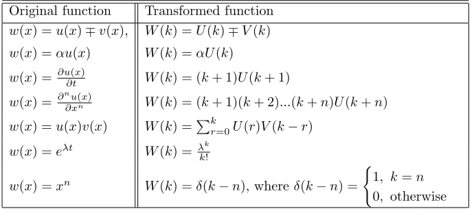
The fundamental mathematical operations performed by one dimensional differen-tial transform method can readily be obtained and are listed in Table 1.
Here, we propose a new idea in order to use the DTM to solve optimization problem (3.2) with constrain (3.1). We consider the the following initial value problem (IVP)
˙
x=f(t, x(t))−g(t, x(t))R−1gT(t, x(t))p(t),
˙
p=−
(
Qx(t) + (∂f(t,x∂x(t)))Tp(t) +∑ni=1pi(t)[−R−1gT(t, x(t))p(t)]T ∂gi(∂xt,x(t))
) ,
x(t0) =x0, p(t0) =α,
(4.6)
αand then the optimal pair (x(.), u(.))T is immediately given. A similar procedure is done to solve problem (2.3) with respect to (2.1) and (2.2), where the imposed boundary condition is given by (2.11).
Table 1. The operations for the one-dimensional differential transform method.
Original function Transformed function
w(x) =u(x)∓v(x), W(k) =U(k)∓V(k)
w(x) =αu(x) W(k) =αU(k)
w(x) =∂u∂t(x) W(k) = (k+ 1)U(k+ 1)
w(x) =∂n∂xu(nx) W(k) = (k+ 1)(k+ 2)...(k+n)U(k+n)
w(x) =u(x)v(x) W(k) =∑kr=0U(r)V(k−r)
w(x) =eλt W(k) =λk
k!
w(x) =xn W(k) =δ(k−n),whereδ(k−n) =
{
1, k=n
0, otherwise
According to the above discussions, the following theorem can be stated:
Theorem 4.3. Consider the OCP of the nonlinear system in (3.1) with performance index in (3.2). Employing the DTM, the optimal pair(x(.), u(.))T is given as follows
{
x∗(t) =∑∞k=0X(k)tk, t∈[t
0, tf],
u∗(t) =−R−1gT(t, x∗(t))∑∞k=0P(k), t∈[t0, tf].
(4.7)
A similar theorem can be concluded for linear system (2.1)-(2.2) with the quadratic performance index (2.3).
5. Application of the DTM for non-linear OCP’s
In this section, we propose a practical implementation to design the suboptimal control to system (3.1) with cost function (3.2). For the linear-quadratic problem (2.3) with constrains (2.1) and (2.2) the strategy is similar.
It is clearly impossible to obtain the optimal trajectory and the optimal control law as in (4.7), since it contains infinite series. In practice, the Nth order suboptimal trajectory-control pair is obtained by replacing∞with a finite positive integerN in (4.7) as follows:
{
xN(t) =∑Nk=0X(k)tk,
uN(t) =−R−1gT(t, xN(t))∑N
k=0P(k)t
k. (5.1)
accuracy if for a given positive constantϵ >0,the following condition holds:
|J(N)−J(N−1)
J(N) |< ϵ, (5.2)
where
J(N)=1 2
∫ tf
t0 (
(x(N)(t))TQx(N)(t) + (u(N)(t))TRu(N)(t)
)
dt. (5.3)
If the tolerance error boundϵ >0 be chosen small enough, the Nth-order suboptimal trajectory-control law will be very close to the optimal pair (x∗(t), u∗(t))T,the value of performanceJ(N)in (5.3) will be very close to its optimal valueJ∗ and the boundary
conditions will be tightly satisfied.
6. Simulation results
In this section we present some numerical examples to illustrate the proposed method.
Example 6.1: [11]
minJ =
∫ 1
0
u2(t)dt
subject to
{
˙
x= 12x2(t) sinx(t) +u(t), t∈[0,1], x(0) = 0, x(1) = 0.5 .
According to the PMP, the following nonlinear 2PBVP is obtained
˙
x= 1 2x
2(t) sinx(t)−1
2p(t), t∈[0,1],
˙
p=−p(t)x(t) sinx(t)−12p(t)x2(t) cosx(t), t∈[0,1], x(0) = 0, x(1) = 0.5,
(6.1)
and the optimal control law is given by
u(t) =−1
2p(t). (6.2) We consider the following IVP
˙
x= 12x2(t) sinx(t)−12p(t), t∈[0,1],
˙
p=−p(t)x(t) sinx(t)−12p(t)x2(t) cosx(t), t∈[0,1],
x(0) = 0, p(0) =α.
(6.3)
According to the DTM for (6.3) by an iterative procedure, we obtain the following components
(k+ 1)X(k+ 1) = 12(∑kr=0∑rs=0X(s)X(r−s)U(k−r)−P(k)
) ,
(k+ 1)P(k+ 1) =∑kr=0∑rs=0P(s)X(r−s)U(k−r)−
1 2 (∑k r=0 ∑r s=0 ∑s
p=0P(p)X(s−p)X(r−s)V(k−r) )
,
X(0) = 0, P(0) =α,
whereU andV are the DTM of sin(x) and cos(x) as follows
U(0) = sin(0);V(0) = cos(0), U(k) =∑ki=0−1[kk−iV(i)X(k−i)],
V(k) =−∑ki=0−1[k−kiU(i)X(k−i)].
(6.5)
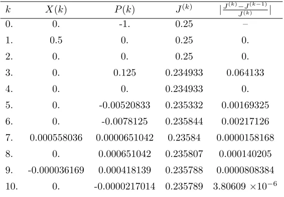
Table 2. Simulation results of the proposed method in different iteration times for Example 6.1.
k X(k) P(k) J(k) |J(k)−J(k−1)
J(k) |
0. 0. -1. 0.25 –
1. 0.5 0. 0.25 0.
2. 0. 0. 0.25 0.
3. 0. 0.125 0.234933 0.064133
4. 0. 0. 0.234933 0.
5. 0. -0.00520833 0.235332 0.00169325
6. 0. -0.0078125 0.235844 0.00217126
7. 0.000558036 0.0000651042 0.23584 0.0000158168
8. 0. 0.000651042 0.235807 0.000140205
9. -0.000036169 0.000418139 0.235788 0.0000808384
10. 0. -0.0000217014 0.235789 3.80609×10⁻⁶
In order to obtain a suboptimal trajectory-control pair with remarkable accuracy, we use the proposed guideline in Section 5 with the tolerance error boundϵ= 5×10⁻⁵.
Substituting (6.5) into (6.4) and after some manipulations, we acquire|J(10)J(10)−J(9)|=
3.80609×10⁻⁶< ϵ; where by imposing the boundary conditionx10(1) = 0.5,we have ∑10
k=0X(k) = 0.5 i.e. α=−0.998958≃ −1. Thus we obtain
x(t) =1 2t,
and from (6.2)
u(t) =−1 2
10 ∑
k=0
p(k) = 1 2−
t3
16+
t5
384+
t6
256 −
t7
30720 −
t8
3072−
t9
4783+
t10
92160.
Example 6.2: [11]
minJ =1 2x
2
(1) +1 2
∫ 1
0
(x2(t) +u2(t))dt,
subject to
{
˙
x=−2x(t) +u(t)
x(0) = 1, x(1) is free.
The exact solution ofk(t) is
k(t) =
√
5 cosh√5(1−t)−sinh√5(1−t)
√
5 cosh√5(1−t) + 3 sinh√5(1−t). (6.6)
We solve the following IVP
˙
x=−2x(t)−p(t),
˙
p=−x(t) + 2p(t),
x(0) = 1, p(0) =α.
(6.7)
Implementing the DTM for (6.7) we have
(k+ 1)X(k+ 1) =−2X(k)−P(k),
(k+ 1)P(k+ 1) =−X(k) + 2P(k),
X(0) = 1, P(0) =α.
(6.8)
We select the tolerance error boundϵ= 5×10⁻⁵and get|J(12)−J(11)
J(12) |= 0.0000272704< ϵ; where by employing the boundary condition x12(1)−p12(1) = 0, we have α =
0.243534.Therefore using (2.15) we have
k(t) =
∑12
k=0P(k)t
k
∑12
k=0X(k)tk
, (6.9)
Table 3. Simulation results of the proposed method in different iteration times for Example 6.2.
k X(k) P(k) J(k) |J(k)−J(k−1)
J(k) |
0. 1. 0.243534 1.02965 –
1. -2.24353 -0.512933 1.00137 0.0282411
2. 2.5 0.608834 1.08208 0.0745874
3. -1.86961 -0.427444 0.310381 2.48631
4. 1.04167 0.253681 0.224674 0.381468
5. -0.467403 -0.106861 0.116038 0.936216
6. 0.173611 0.0422801 0.127557 0.0903023
7. -0.0556432 -0.0127215 0.120514 0.0584406
8. 0.015501 0.00377501 0.122105 0.0130347
9. -0.00386411 -0.000883441 0.121693 0.00339046
Figure 1. Comparison of the exact solution ofk(t) with the DTM solution in Example 6.2.
0.0 0.2 0.4 0.6 0.8 1.0
0.3 0.4 0.5 0.6 0.7 0.8 0.9 1.0
t
k
H
t
L
DTM solution Exact solution
Example 6.3: [11]
minJ =1 2
∫ 1
0
(x2(t) +u2(t))dt
subject to
{
˙
x=−x(t) +u(t), x(0) = 1, x(1) is free.
The exact solution ofk(t) is
k(t) =−(1 +
√
2β) cosh(√2t) + (√2 +β) sinh(√2t)
where
β=−cosh(
√
2) + (√2) sinh(√2)
√
2 cosh(√2) + sinh(√2) . (6.11)
We consider
˙
x=−x(t)−p(t),
˙
p=−x(t) +p(t),
x(0) = 1, p(0) =α.
(6.12)
Implementing the DTM for (6.12) we have
(k+ 1)X(k+ 1) =−X(k)−P(k) (k+ 1)P(k+ 1) =−X(k) +P(k),
X(0) = 1, P(0) =α.
(6.13)
Table 4. Simulation results of the proposed method in different iteration times for Example 6.3.
k X(k) P(k) J(k) |J(k)−J(k−1)
J(k) |
0. 1. 0.385819 0.574428 –
1. -1.38582 -0.614181 0.145989 2.93473
2. 1. 0.385819 0.238132 0.386938
3. -0.46194 -0.204727 0.184162 0.293056
4. 0.166667 0.0643032 0.195237 0.0567272
5. -0.046194 -0.0204727 0.192453 0.0144678
6. 0.0111111 0.00428688 0.192989 0.00277637
7. -0.00219971 -0.00097489 0.192897 0.000477353
8. 0.000396825 0.000153103 0.192911 0.0000746814
9. -0.0000611031 -0.0000270803 0.192909 0.0000102555
We select the tolerance error bound ϵ = 5 ×10⁻⁵ and acquire |J(9)−J(8) J(9) | =
0.0000102555 < ϵ; where by employing x9(1)−p9(1) = 0, we get α = 0.385819.
Therefore we have
k(t) =
∑9
k=0P(k)t
k
∑9
k=0X(k)tk
, (6.14)
Figure 2. Comparison of the exact solution ofk(t) with the DTM solution in Example 6.3.
0.0 0.2 0.4 0.6 0.8 1.0
0.0 0.1 0.2 0.3
t
k
H
t
L
DTM solution Exact solution
Example 6.4: [26]
minJ =1 2Sx
2
(15) +1 4
∫ 15
0
u2(t)dt
subject to
{
˙
x=−0.2x(t) +u(t),
x(0) = 5, x(15) is free, S >0.
The optimal control low isu(t) =−2K(t)x(t) where
K(t) = [e0.2(tf−t)+ S 0.2[e
0.2(tf−t)−e−0.2(tf−t)]]−1[Se−0.2(tf−t)].
From equation (9), we consider
˙
x(t) =−0.2x(t)−2p(t),
˙
p(t) = 0.2 p(t), x(0) = 1, p(0) =α.
(6.15)
Employing the DTM for (6.15) we have
X(k) = 1k(−0.2X(k−1)−2P(k−1)), P(k) = 1
k(0.2P(k−1)),
X(0) = 1, P(0) =α.
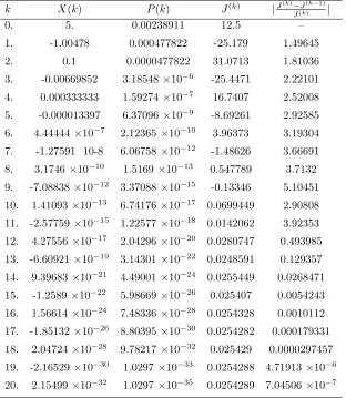
Table 5. Simulation results of the proposed method in different iteration times for Example 6.4.
k X(k) P(k) J(k) |J(k)−J(k−1)
J(k) |
0. 5. 0.00238911 12.5 –
1. -1.00478 0.000477822 -25.179 1.49645
2. 0.1 0.0000477822 31.0713 1.81036
3. -0.00669852 3.18548×10⁻⁶ -25.4471 2.22101
4. 0.000333333 1.59274×10⁻⁷ 16.7407 2.52008
5. -0.000013397 6.37096×10⁻⁹ -8.69261 2.92585
6. 4.44444×10⁻⁷ 2.12365×10⁻¹⁰ 3.96373 3.19304
7. -1.27591 10-8 6.06758×10⁻¹² -1.48626 3.66691
8. 3.1746×10⁻¹⁰ 1.5169×10⁻¹³ 0.547789 3.7132
9. -7.08838×10⁻¹² 3.37088×10⁻¹⁵ -0.13346 5.10451
10. 1.41093×10⁻¹³ 6.74176×10⁻¹⁷ 0.0699449 2.90808
11. -2.57759×10⁻¹⁵ 1.22577×10⁻¹⁸ 0.0142062 3.92353
12. 4.27556×10⁻¹⁷ 2.04296×10⁻²⁰ 0.0280747 0.493985
13. -6.60921×10⁻¹⁹ 3.14301×10⁻²² 0.0248591 0.129357
14. 9.39683×10⁻²¹ 4.49001×10⁻²⁴ 0.0255449 0.0268471
15. -1.2589 ×10⁻²² 5.98669×10⁻²⁶ 0.025407 0.0054243
16. 1.56614×10⁻²⁴ 7.48336×10⁻²⁸ 0.0254328 0.0010112
17. -1.85132×10⁻²⁶ 8.80395×10⁻³⁰ 0.0254282 0.000179331
18. 2.04724×10⁻²⁸ 9.78217×10⁻³² 0.025429 0.0000297457
19. -2.16529×10⁻³⁰ 1.0297×10⁻³³ 0.0254288 4.71913×10⁻⁶
20. 2.15499×10⁻³² 1.0297×10⁻³⁵ 0.0254289 7.04506×10⁻⁷
Settingϵ= 5×10⁻⁵we obtain|J(20)−J(19)
J(19) |= 7.04506×10−
7< ϵ; where by using the
boundary conditionSx(t)−p(t) = 0,we have
α= 0.00238911, forS= 5, α= 0.00177368, forS= 0.5, α= 0.000495996, forS= 0.05.
(6.17)
Therefore
k(t) =
∑20
k=0P(k)t
k
∑20
k=0X(k)tk
, (6.18)
(x(.), u(.))T are also shown in Figures 4 and 5. One can compare these approximate results with the exact results in [26] page 213.
To end this section, we answer a natural question: Are there advantages of the proposed collocation method compared to the existing ones? To answer this, we summarize what we have observed from numerical experiments and theoretical results as below.
• The technique that we used, which is based on Taylor series expansion enables us to obtain a series solution by means of an iterative procedure.
•The main advantage of the method is the fact that it provides its user with an analytical approximation, in many cases an exact solution, in a rapidly convergent sequence with elegantly computed terms.
•A specific advantage of this method over any purely numerical method is that it offers a smooth, functional form of the solution over a time step.
• The other advantages of this method, compared to other analytic methods are controllable accuracy, and high efficiency which is exhibited by the rapid convergence of the solution.
•This method can be applied directly to differential equations without requiring linearization, discretization or perturbation.
•Large computational work and roundoff errors are avoided.
•All the calculations in the method are very easy.
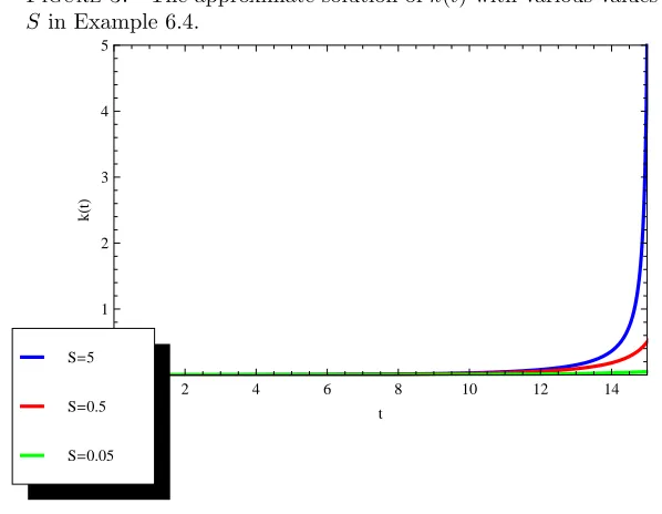
Figure 3. The approximate solution ofk(t) with various values of
S in Example 6.4.
0 2 4 6 8 10 12 14
0 1 2 3 4 5
t
k
H
t
L
S=0.05
S=0.5
Figure 4. The approximate solution ofx(t) with various values of
S in Example 6.4.
0 2 4 6 8 10 12 14
0 1 2 3 4 5
t
x
H
t
L
S=0.05
S=0.5
S=5
Figure 5. The approximate solution ofu(t) with various values of
S in Example 6.4.
0 2 4 6 8 10 12 14
-0.12
-0.10
-0.08
-0.06
-0.04
-0.02
0.00
t
u
H
t
L
S=0.05 S=0.5 S=5
7. Conclusion
Applying the DTM, the optimal control law and the corresponding optimal trajec-tory are determined in the form of rapid convergent series with easy computable terms. The present study has confirmed that the DTM offers great advantages of straightforward applicability, computational efficiency and high accuracy. The Differ-ential transform method needs less work in comparison with the traditional methods. Therefore, this method can be applied to many complicated linear and non-linear problems and does not require linearization, discretization or perturbation. More-over, in view of computational complexity, the proposed method is more practical than the other approximate approaches. Mathematica and Matlab have been used for computations and simulations in this paper.
References
[1] M. Abu-Khalaf, J. Huang, and F. L. Lewis,NonlinearH2/H∞Constrained Feedback Control, a Practical Design Approach Using Neural Networks, Springer-Verlag, NewYork., (2006). [2] A. K. Alomari, A new analytic solution for fractional chaotic dynamical systems using the
differential transform method, Computers & Mathematics with Applications.,61(2011),
2528-2534.
[3] U. M. Ascher, R. M. M. Mattheij, and R.D. Russel,Numerical solution of bound- ary value
problems for ordinary differential equations, SIAM, Philadelphia., (1995).
[4] S. P. Banks and K. Dinesh,Approximate optimal control and stability of nonlinear finite–and
infinite-dimensional systems, Annals of Operations Research.,98(2000), 19-44.
[5] V. L. Baranov, Solution of nonlinear boundary value problems on the basis of differential
transforms, Engineering Simulation.,14(1997), 599–608.
[6] R. W. Beard, G. N. Saridis, and J. T. Wen,Galerkin approximations of the generalized
Hamil-tonJacobiBellman equation, Automatica.,33(1997), 2159-2177.
[7] R. Bellman,On the theory of dynamic programming, PNAS.,38(1952), 716–719.
[8] A. E. Bryson,Applied Linear Optimal Control: Examples and Algorithms, Cambridge Univer-sity Press, UK., (2002).
[9] T. Cimen, State dependent Riccati equation (SDRE) control: a survey, 17th IFAC World
Congress, Seoul, Korea.(2008).
[10] O. Demirdag and Y. Yesilce,Solution of free vibration equation of elastically supported
Tim-oshenko columns with a tip mass by differential transform method, Advances in Engineering
Software.,42(2011), 860-867.
[11] S. Effati and H. Saberi Nik,Solving a class of linear and non-linear optimal control problems
by homotopy perturbation method,28(2011), 539–553.
[12] A. Elsaid,Fractional differential transform method combined with the Adomian polynomials, Applied Mathematics and Computation.,218(2012), 6899-6911.
[13] V. S. Ert¨urk and S. Momani,Differential transform technique for solving fifth-order boundary
value problems, Mathematical and Computational Applications.,13(2008), 113–121.
[14] W. L. Garrard and J. M. Jordan,Design of nonlinear automatic flight control systems,
Auto-matica.,13(1997), 497-505.
[15] H. P. Geering, Optimal Control with Engineering Applications, Berlin: Springer., (2007). [16] A. G¨okdoˇgan, M. Merdan, and A. Yildirim,The modified algorithm for the differential
trans-form method to solution of Genesio systems, Communications in Nonlinear Science and
Nu-merical Simulation.,17(2012), 45-51.
[17] P. K. Gupta,Approximate analytical solutions of fractional BenneyLin equation by reduced
dif-ferential transform method and the homotopy perturbation method, Computers & Mathematics
with Applications.,61(2011), 2829-2842.
[18] S. Haq, S. Islam, and J. Ali,Numerical solution of special 12th-order boundary value problems
using differential transform method, Communications in Nonlinear Science and Numerical
[19] S. Hesam, A. R. Nazemi, A. Haghbin, Analytical solution for the generalized Kuramoto–
Sivashinsky equation by differential transform method, Scientia Iranica, Transactions B:
Me-chanical Engineering.20(2013), 1805–1811.
[20] S. Hesam, A. R. Nazemi, and A. Haghbin,Analytical solution for the Fokker-Planck equation
by differential transform method, Transactions B: Mechanical Engineering.19 (4)(2012), 1140–
1145.
[21] J. Huang and C. F. Lin,Numerical approach to computing nonlinear H-infinity control laws, Journal of Guidance, Control, and Dynamics.,18 (1995), 989–994.
[22] H. Jaddu and E. Shimemura,Computational method based on state parameterization for
solv-ing constrained nonlinear optimal control problems,International Journal of Systems Science.,
30(1999), 275-282.
[23] A. Jajarmi, N. Pariz, A. Vahidian, and S. Effati,A Novel Modal Series Representation
Ap-proach to Solve a Class of Nonlinear Optimal Control Problems, International Journal of
Innovative Computing, Information and Control.,7(2011), 501–510.
[24] R. E. Kalman,Contributations to the theory of optimal control, Boletin de la Sociedad Matem-atica Mexicana., (1960), 102–119.
[25] M. Keimanesh, M. M. Rashidi, A. J. Chamkha, and R. Jafari, Study of a third grade non-Newtonian fluid flow between two parallel plates using the multi-step differential transform
method, Computers & Mathematics with Applications.,62(2011), 2871-2891.
[26] D. E. Kirk, Optimal Control Theory: An Introduction, Prentice Hall, Englewood Cliff, New Jersey., (1970).
[27] J. Liu and G. Hou,Numerical solutions of the space- and time-fractional coupled Burgers
equa-tions by generalized differential transform method, Applied Mathematics and Computation.,
217(2011), 7001-7008.
[28] V. Manousiouthakis and D. J. Chmielewski,On constrained infinite-time nonlinear optimal
control, Chemical Engineering Science.,57(2002), 105-114.
[29] S. Momani and V. S. Ert¨urk,Solving a system of fourth-order obstacle boundary value problems
by differential transform method, Kybernetes.,37(2008), 315–325.
[30] T. Notsu, M. Konishi, and J. Imai,Optimal water cooling control for plate rolling, International Journal of Innovative Computing Information and Control.,4(2008), 3169-3181.
[31] L. S. Pontryagin, V. G. Boltyanskii, R. V., Gamkrelidze, and E. F. Mishchenko,The
Mathe-matical Theory of Optimal Processes, Wiley Interscience Publishers, New York., (1962).
[32] J. E. Rubio,Control and Optimization; The Linear Treatment of Non-linear Problems, Manch-ester, U. K., Manchester University Press., (1986).
[33] G. Y. Tang,Suboptimal control for nonlinear systems, a successive approximation approach, Systems & Control Letters.,54(2005), 429-434.
[34] L. Tang, L. D. Zhao, and J. Guo,Research on pricing policies for seasonal goods based on
optimal control theory., ICIC Express Letters,3(2009), 1333-1338.
[35] A. Tari and S. Shahmorad,Differential transform method for the system of two-dimensional
nonlinear Volterra integro-differential equations, Computers & Mathematics with
Applica-tions.,61(2011), 2621-2629.
[36] S. A. Yousefi, M. Dehghan, and A. Lotfi, Finding the optimal control of linear systems via
Hes variational iteration method,International Journal of Computer Mathematics.,87(2010),
1042-1050.