Improving Performance of Spatial Network Queries

(1)

University of New Orleans University of New Orleans

ScholarWorks@UNO

University of New Orleans Theses and

Dissertations Dissertations and Theses

8-9-2006

Improving Performance of Spatial Network Queries

Elias Ioup

University of New Orleans

Follow this and additional works at: https://scholarworks.uno.edu/td

Recommended Citation Recommended Citation

Ioup, Elias, "Improving Performance of Spatial Network Queries" (2006). University of New Orleans Theses and Dissertations. 406.

https://scholarworks.uno.edu/td/406

This Thesis is protected by copyright and/or related rights. It has been brought to you by ScholarWorks@UNO with permission from the rights-holder(s). You are free to use this Thesis in any way that is permitted by the copyright and related rights legislation that applies to your use. For other uses you need to obtain permission from the rights-holder(s) directly, unless additional rights are indicated by a Creative Commons license in the record and/or on the work itself.

(2)

Improving Performance of Spatial Network Queries

A Thesis

Submitted To The Graduate Faculty of the University of New Orleans

in partial fulfillment of the requirements for the degree of

Master of Science in

Computer Science

by

Elias Zayd Khalil Ioup

B.S., University of Chicago, 2003

(3)

Acknowledgements

I would like to thank Olivier Tabone and Olivier Mansion of Ecole Centrale, Nantes, France for their invaluable work in implementing much of this project. Thanks to the Department of Computer Science for funding and housing this project and providing the equipment necessary to complete it. I would also like to thank Kevin Shaw and John Sample of the Naval Research Laboratory at

(4)

Abstract

Spatial network queries, for example KNN or range, operate on systems where objects are constrained to

locations on a network. Current spatial network query algorithms rely on forms of network traversal which

have a high complexity proportional to the size of the network making, them poor for large real-world

networks. In this thesis, an alternative method of approximating the results of spatial network queries with

a high level of accuracy is introduced. Distances between network points are stored in an M-Tree index, a

balanced tree index where metric distance determines data ordering. The M-Tree uses the chessboard

metric on network points embedded in a higher dimensional space using tRNE. Using the M-Tree both

KNN and range queries are computed more efficiently than network traversal. Error rates of the M-Tree are

low, with accuracies of 97% possible on KNN queries and perfect accuracy with 2% extra results on range

(6)

Introduction

Work on spatial databases has been extensive over the years. However, the work

has for the most part been limited to systems where objects may be located anywhere on

the Euclidean plane. Just as important are systems where objects are limited to locations

on a network such as roads or rivers. The problems and solutions involved in these

systems are very different from Euclidean systems. Managing large spatial network

databases requires developing separate solutions.

Network expansion is the most common method of performing queries in a spatial

network. The network expansion algorithm is a modification to Dijkstra's algorithm for

searching a graph; it travels the network from a query point until it collects all results to a

query. The problem with the network expansion algorithm is its complexity. It has

complexity proportional to the number of nodes in the network and is slow for large

networks common in spatial network queries (such as a road network). Little can be done

to improve the algorithm because of its underlying requirement of network traversal.

Other methods must be explored.

One such method is to modify the underlying network data. Reducing the

number of nodes in the network will have a substantial effect in increasing the

performance of the network expansion algorithm. Node reduction can be accomplished

by identifying nodes which do not describe connectivity within the network and

removing them. It is also possible to increase the speed of data access. Reducing the

(7)

performance of network expansion, the underlying problems of network expansion are

unchanged. Fixing such problems requires a different approach.

Indexing is one method of reducing algorithm times for spatial network queries.

However, indexing data in spatial networks has not differed much from indexing normal

spatial data. R-Tree indexes are the basis for most methods to index spatial networks.

The difficulty in R-Tree indexes is that data is organized strictly on Euclidean distance

between objects rather than network distance. Euclidean distance is a poor

approximation for network distance. Using an R-Tree to index data in a spatial network

invariably has problems.

An M-Tree index is a better data organization method for spatial network data.

The M-Tree organizes data according to any arbitrary metric. In the case of a spatial

network, the metric is the network distance between objects in the network. The M-Tree

is designed to perform similarity queries such as KNN and range queries, i.e. just the

queries necessary in spatial networks.

The only difficulty with an M-Tree index is that it requires a method of

computing distance in the network which is efficient. In performing KNN and range

queries the M-Tree requires many network distance computations. If these distance

computations are slow then the M-Tree is of no benefit in performing similarity queries

in a network.

There are several different methods of computing distance in a network which

may be used with the M-Tree. These include Dijkstra’s algorithm, A* search, hill

(8)

obstacles to its usage with the M-Tree. In the end, these methods do not offer the

performance required to be effective when used with the M-Tree.

The solution to the distance computation problem is to use a distance metric as

easy to compute as Euclidean distance. The coordinates of the network objects can be

transformed into a higher dimensional space, a process called Road Network Embedding

(RNE) [1]. An LP metric in the embedded space is an accurate approximation of true

network distance. LP distance is a simple computation which can be performed quickly.

When the M-Tree performs similarity queries it can use this new distance metric. The

increased speed of the embedded distance computation is passed on to the query

evaluation.

The main contribution of this thesis is to introduce improved methods of

computing spatial network queries. First, data manipulation which improves the

performance of network queries and network preprocessing is introduced. Network

pruning reduces the number of nodes in the network, thereby increasing the performance

of algorithms dependent on node complexity. Secondly, the M-Tree is introduced as an

access method for spatial network data. The M-Tree is an innovative way of performing

spatial network queries which previously were performed by network traversal

algorithms. To the best of our knowledge, the M-Tree has never before been used to

perform spatial network queries because integrating the M-Tree with a network distance

is difficult. Road Network Embedding provides an efficient method of computing

network distance which works perfectly with the M-Tree. By combining the M-Tree with

(9)

The M-Tree is both a fast and versatile access method which outperforms current

algorithms for computing spatial network queries.

The M-Tree with the embedded network is more efficient than other methods of

performing KNN and range queries. Network expansion [2] is the most used method of

performing these queries. Compared to a standard implementation of network expansion

with a database stored network, the M-Tree shows better performance for all size queries.

For range queries the M-Tree is anywhere from 7 to 28 times fasters. KNN queries are

up to 45 times faster for smaller values of k. The speed increase over network expansion

grows even faster for larger values of k. The M-Tree not only outperforms network

expansion but in many cases other methods as well. The M-Tree’s increase in

performance over network expansion is often much greater than that of Network Voronoi

diagrams [3]. The M-tree is also a more versatile access method than Network Voronoi

diagrams. While the Voronoi diagrams only support KNN queries, the M-Tree supports

both KNN and range queries, the two most common types of spatial network queries.

First, this paper discusses previous work performing spatial network queries and

explains the network model and queries which are used later. Then the M-Tree is

introduced as a solution to evaluating KNN and range queries. After comparing different

possible methods of computing network distance, we introduce truncated Road Network

Embedding (tRNE) which allows efficient computation of network distance. The M-Tree

with tRNE is compared to network expansion and shown to have better performance

when computing KNN, range, and Aggregate KNN (AKNN) queries. The latter query is

a good example of the versatility of the M-Tree. While network expansion works well in

(10)

complex queries like AKNN. The M-Tree does adapt well to these more complicated

(11)

Background

Papadias et al. [2] created a comprehensive approach to querying spatial network

databases. They suggest two general methods for performing KNN and range queries.

The first is Euclidean restriction. This method exploits the fact that the network distance

to a point is always greater than or equal to the Euclidean distance. The other method is

network expansion. Network expansion is the faster algorithm and is used in other

spatial network queries, such as the moving object KNN query by Jensen et al. [4]. It is

also the benchmark used to compare to other spatial network query algorithms, such as

the Voronoi based KNN query introduced by Kolahdouzan and Shahabi [3].

Network expansion works by traversing the network from the initial query point,

similar to Dijkstra’s algorithm. As it traverses the network the algorithm adds points of

interest that match the query as it reaches them. For KNN queries the algorithm

continues until K points have been retrieved. For range queries the algorithm continues

until all segments within the given range are traversed. Like Dijkstra’s algorithm,

network expansion has complexity dependent on the number of nodes and edges in the

network.

The data in the network is indexed using an R-Tree. Both segments and the

points of interest are indexed in an R-Tree. The points of interest (POI) on the network

are not actually connected to the network. POI are linked to the correct segments on the

network using the Tree. Other than finding initial locations and linking POI, the

R-Tree is not used in the network expansion algorithm.

Kolahdouzan and Shahabi [3] created a method of solving KNN network queries

(12)

regions which are closest in network distance to the various points of interest. By

precomputing the diagram, they provide an efficient method of performing K nearest

neighbor queries. Finding the KNN involves finding the Voronoi cell that contains the

query point. The next nearest neighbors are in the adjacent cells. Continually visiting the

adjacent cells provides as many nearest neighbors as necessary. The network Voronoi

cells are indexed by an R-Tree, allowing fast searching for particular cells.

While they are between 1.5 and 12 times faster than network expansion, Voronoi

diagrams are used for solving KNN queries only. Network expansion is useful for other

types of queries, such as range queries. This method, while making traversing the

network much more efficient, does require a form of network search. Despite the fact

that the search is over Voronoi cells, the performance will still be highly sensitive to the

size of the query.

As in the above research, the R-Tree is the standard method of indexing the

spatial networks. In addition to the above, Pfoser and Jensen [5] as well as Jensen et al.

[4] use the R-Tree to index networks. The difficulty of an R-Tree is that it is designed for

unconstrained spatial queries, not network constrained spatial queries. The network

Voronoi diagram and network expansion are two methods designed to overcome the

difficulties of this index. However, it would be desirable to instead have another type of

index made to work with the constraints imposed by a spatial network. The M-Tree

index is such a data structure.

An example of a more complex spatial network query is an Aggregate KNN

(13)

distances from each query point to each point of interest. Liu et al. [6] survey algorithms

to solve the AKNN query over networks and find Incremental Euclidean Restriction

(IER) to be the best. This algorithm retrieves the Euclidean nearest neighbors of the

query points and then computes the actual network distances to these preliminary results

to determine the AKNN. While the network distance computation is an optimized

version of the A* search algorithm, this algorithm still requires a large number of

network traversals which are expensive. The benefit of the M-Tree is that more complex

(14)

Proposed Methodology

Network Model

A real world spatial network such as a system of roads must be modeled for use in

a database. This network model approximates the network in 2 dimensions. Often this

approximation is termed 1.5 dimensions because objects and motion are strictly located

on the 1 dimensional network lines which move in 2 dimensions.

A spatial network is made up of network segments and network nodes. A node

exists wherever a road ends or two roads intersect. The nodes separate the roads into

segments. The portion of a road between two nodes is defined as one segment. Segments

are the basic type of the network. Each segment is defined as a polyline. A polyline L is

a sequence of points:

!

L"(p1,p2,...,pn) where

!

pi" #

2

A node N in the network is represented as:

!

N"pi# $

2 where

!

pi"{p1,pn}

Nodes indicate all the connections between road segments and therefore indicate

how travel can take place in the network. If two road segments do not share a node then

they do not directly connect. The network segments are assumed to be bidirectional as in

other network models [4][3][5][6]. The network is then a metric space and has many

useful properties.

Spatial Network Queries

(15)

a certain range from a given query point. Below is a formal definition of a range query

R(p,ρ):

!

R(p,")={o#M|d(p,o)$"}

M = points of interest

p = query point

d(x,y) = distance over network from point x to y

!

" = max distance from the query point

The KNN query returns the k closest objects to the query point. Below is the definition of

a KNN query:

!

KNN={N"M|N =k# $o%N,q&N'd(p,o)>d(p,q)}

k = number of objects to return

A third query, Aggregate KNN, is an example of a more complex spatial network query.

The AKNN query returns the k "closest" objects to multiple query points. Closest is

defined as the shortest aggregate distance from each of the query points. The aggregate

distance is computed by applying a user defined aggregate function to the distance to

each query point. Any aggregate function, such as the sum or max, can be used in

conjunction with the AKNN query. The formal definition of the AKNN query is below:

!

AKNN={N"M|N =k# $o%N,q&N'dagg(P,o)>dagg(P,q)}

k = number of objects to return

P = set of query points

(16)

Graph Processing

The Data Set

The actual data for the spatial network may come in many different forms. For

this research, TIGER data from the US Census was used as the underlying network. The

primary reason for using this specific data set is that it is free to the public and provides

the road network for the entire United States. For these experiments, however, only two

states were used, Louisiana and California.

Another possible source of spatial network data is provided by companies such as

Navtech and TeleAtlas. The data provided by these companies is more accurate and

better formatted for use in actual spatial network applications. However, these data sets

are expensive and thus not available for this work. The methods described here are

applicable to these commercial data sets as well as to other spatial networks which are

not roads.

Graph Creation

The initial network data is organized as network segments which are encoded as a

sequence of latitude and longitude coordinates. First, the two endpoints of each network

segment are created as nodes in the network graph. In this system, the points of interest

are also included as nodes in the graph. Including points of interest as nodes in the graph

is not necessary to the graph processing described below. Often the points of interest are

too dynamic a set to hard code them into the graph. If points of interest are not included

as nodes, it is required that they be explicitly linked to the network segment on which

(17)

The graph is stored as a sequence of adjacency lists, one for each node. The

following information is stored in the graph for each node in the network:

1. The id of the node.

2. The coordinates of the node.

3. The number of adjacent nodes.

4. An array of references to adjacent nodes.

5. The distance to each adjacent node.

6. A reference to point of interest information if this node is a point of interest.

The above fields must be updated as the graph is processed. Below are the important

changes that are made to the graph of the network.

The original network data may not necessarily ensure correct connectivity

between network segments. Two segments which are connected in the real world may

have endpoints whose coordinates are slightly different. These nodes should have the

same coordinates and be labeled as the same node. All nodes should be compared to

ensure that small decimal errors do not differentiate nodes which should be the same. An

R-Tree over the node coordinates will allow efficient search for nodes which should be

merged. It is essential that the network segments be updated with new node equivalences

to ensure that connectivity information is preserved.

After all the nodes are determined the graph is pruned of unessential nodes and

segments [7]. Nodes and line segments which contain points of interest will not be

pruned. These sections of the graph contain the information important to the network

queries and must stay intact. Jensen et al. [4] proposed such a technique and removed all

(18)

because these nodes do not model connectivity to an alternate path. Collapsing these

segments into one segment cannot alter possible paths taken by a graph traversal

algorithm.

Nodes with one adjacency may also be removed from the graph. It is these nodes

which often allow the greatest amount of pruning to be performed. These nodes represent

end sections of the graph which contain no useful information to answer queries and no

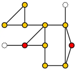
connectivity information. Figures 1 through 3 show an example of nodes pruned from a

graph. Yellow nodes are regular graph nodes. The red nodes are points of interest and

are exempt from the pruning requirements. In Figure 1, the nodes with one adjacency are

removed from the network. Figure 2 shows nodes with two adjacencies pruned. The

final network with all nodes removed is shown in Figure 3.

The resultant graph after pruning will have fewer nodes and line segments. Most

queries on the pruned graph will run faster because their complexity is based on the

number of nodes or line segments in the graph.

(19)

Figure 2. Remove nodes with two adjacencies (dashed nodes). Red nodes are points of interest and left unpruned.

Figure 3. All nodes pruned (dashed nodes) from network. Red nodes are points of interest and left unpruned.

The process of removing nodes is an iterative one. Node are repeatedly removed

from the graph until no remaining nodes fit the pruning categories. The effectiveness of

removing these extra nodes depends on the original network data. Some network data

contains many of these extraneous nodes and segments whereas other data is organized

such that there are no extra line segments. Pruning will be more effective in the former

rather than the latter. Most network data will be reduced in size by pruning, especially

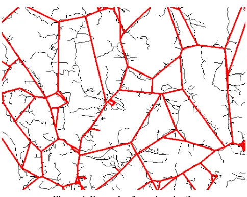
the removal of end nodes. Figure 4 shows an area of roads in Louisiana with the

(20)

Parallelizing the Process

Because removal of nodes is an iterative process, it will take quite a while to

complete on a large and complex network. Running the graph creation in parallel on a

cluster will reduce the required time substantially. The pruning process parallelizes

easily. All slaves are given a copy of the network database. The network is split into

disjoint geographic boxes by the master and assigned to each of the slaves. The slave

removes the unnecessary nodes from its area and sends the changes back to the master.

Once all slaves have finished the current iteration, new work is assigned and the process

repeats until all work is finished. Pseudo code for such an algorithm is shown in Figure

5.

(21)

BEGIN

| work ←next set of id to process | WHILEwork DO

| FOR i=1 Tonslaves STEP 1 DO | | wait for the signal work done of a slave | ENDFOR

END

Figure 5. Algorithm for parallel graph reduction.

Two standard problems when parallelizing a process are how to handle the

boundaries between slave areas and how to limit inter-process communication. Nodes

whose adjacencies are in other slave areas require special handling. Graph changes

during the pruning process necessitate costly communication between the master and the

slaves.

The solution to the boundary problem is to ignore all nodes whose adjacencies are

not in the same area. These nodes are left to be handled by later iterations. After all

slaves have processed their first iteration, the master must redistribute the work. By

changing the location of the boundaries, the probability that a node will be near a

boundary for each iteration is greatly reduced. If any boundary nodes do remain

unhandled at the end of the pruning, the master node will make one final pass over the

entire area and prune the problem nodes. An example of two slave areas is shown in

(22)

Figure 6. Two adjacent slave graph areas. Node N2 is not pruned because its adjacency is in another slave area.

NodesN1/N6 is pruned by slave1/slave2.

To reduce communication within the cluster database updates are made

selectively between the master and slaves. Slaves only send back necessary changes to

the master and the master only updates the necessary portions of the slave database. For

example, if a slave removes four nodes in the current iteration, only the information for

those nodes need be sent back to the master. When assigning work to a slave, only the

area assigned should be updated in the slave’s database. Other areas are not pertinent and

should be left unchanged.

Graph Validation

For complex networks it will be difficult to ensure that the resulting graph is

valid. A validation program checks to ensure correctness in the graph. The following

are properties that should hold in the final graph:

• If A is adjacent to B then B is adjacent to A.

• If A is in the graph then all nodes adjacent to A are in the graph.

(23)

Graph Storage and Access

This section compares two methods of storing and accessing the created graph.

Each method has its benefits and the one selected should be chosen with knowledge

about the network data as well as the application requiring access to the graph.

Database Storage and Access

The first method of graph storage is to use a database. The database provides a

simple method of managing the graph data. This method is highly scalable which is

important when using large network data sets. Accessing the graph is done through basic

database queries. The main concern with this method is how to program the spatial

network queries. The test database used in this project is PostgreSQL [8], but the

techniques apply to most database management systems (DBMS).

Two techniques are possible to access the data from a program implementing

spatial network queries. The first is to have a program external to the database perform

the queries. The benefit of this method is that it is usually easy to write such a program.

The choice of programming languages and tools is wide. Often, there are interfaces that

allow the external program to be accessed from within the database and thus allow the

queries to be used seamlessly. The problem with this method is that database access from

the query program is usually slow. Given that most useful network graphs are fairly large

this is problematic.

The second method to access data from the network queries is to write an

extension to the database. Instead of an external program, the queries are written as

(24)

native database functions. In PostgreSQL this functionality is provided by the Server

Programming Interface (SPI).

SPI is simply a set of native interface functions that allow access to the Parser,

Planner, Optimizer, and Executor of the DBMS. The benefit of SPI (or similar functions

in other DBMS) is that user defined queries are performed fast. There is no connection

overhead or inter-process communication. The downside is that using SPI is more

complex than simply writing an external module. Language choice is limited when

extending the database functionality. SPI is written in C and full access to its

functionality is only available using C (though some other languages provide limited

accessibility). SPI also requires access to data using specific macros, functions, and data

structures which can complicate the writing of functions. However, because SPI is the

fastest method of accessing database data, it is our chosen method of interfacing with the

database. Both KNN and range queries on the spatial network were implemented using

the network expansion algorithm and the Server Programming Interface.

Shared Library Access

The second method of storing and accessing the data is through a dynamically

accessible shared library. A special program generates a C source file containing the

entire structure of the graph. All of the information contained in the database version of

the graph is also contained in the shared library version. There are important benefits to

this method but also some large deficiencies which may preclude its usefulness.

The shared library is actually a hard coded table of nodes. Each node is a global

(25)

number of points of interest. The graph itself is accessed through macros which simplify

the interface and can be used directly through PostgreSQL.

The shared library is modifiable so that the network expansion algorithm can set

flags on particular nodes. These flags indicate containment in particular lists used by the

network expansion algorithm. In addition, the flags record the position of the node in a

particular list. The result is that these lists rarely need to be scanned and the network

expansion algorithm performs more efficiently. A similar fix could be done with the

database access method but the list scan time costs much less than data retrieval and thus

is not a large improvement.

The benefit of the shared library graph is speed. The graph is kept in main

memory and results in extremely fast access times. Applications of spatial network

queries often require speedy results, making the shared library a perfect access and

storage method. Not only is access fast but loading the library is fast. Other main

memory approaches would require loading the library from a data file or database. The

data would need to be parsed and placed in the correct data structures. The shared library

method does not require this startup overhead, making it perfect for an experimental

environment with many tests and restarts. In particular, the shared library provides an

excellent platform for comparing network expansion algorithms to other spatial network

algorithms. The access speed benefit of the shared library approach is matched by other

main memory approaches which may be more suited to an always on, deployed

application.

The problems of the shared library graph, and other main memory approaches, are

(26)

road network covering the entire United States would require about 2-3 gigabytes of main

memory simply to hold the shared library. In addition, compiling the shared library

requires even more memory. Another issue is that the shared library is static. Once

changes are made to the graph the library requires a complete recompilation. Having to

recreate a graph every time one node or segment changes is a significant problem.

These problems are not insurmountable. The memory usage is large but may be

handled with current systems. Large networks may be stored in many shared libraries,

possibly contained on many nodes in a cluster. The static nature of the shared library

approach is not a problem with other main memory approaches which could be used with

dynamic networks. In many cases, spatial networks are static data sets and there is no

need to update the graph on regular intervals.

M-Tree Index

The M-Tree is a tree index structure created by Ciaccia et al. [9]. It is structured

like other database tree indexes such as the B+-Tree and the R-Tree. An M-Tree indexes

data from any metric space. The index is designed to support similarity queries. Unlike

other metric trees the M-Tree is dynamic. Many metric trees organize data according to

absolute distance from a single static object. Instead, the objects in an M-Tree are

organized according to their relative metric distance. Objects which are close in metric

distance are placed near each other in the M-Tree. This property makes the M-Tree

(27)

The M-Tree can index any metric space. A metric space is any set of features

which have a distance defined over them such that the distance satisfies the following

three properties:

• (1) symmetry:

∀ (Ox,Oy) ∈ D2, d(Ox,Oy) = d(Oy,Ox)

• (2) non negativity:

∀ (Ox,Oy) ∈ D2 \ Ox ≠Oy, d(Ox,Oy) > 0 ^ d(Ox,Ox) = 0

• (3) triangle inequality:

∀ (Ox,Oy,Oz) ∈ D3 , d(Ox,Oy) ≤ d(Ox,Oz) + d(Oz,Oy)

The M-Tree is structured much like other database tree indexes. It is a paged and

balanced tree where data is stored at the leaf level. The leaves contain the leaf object Ol

as well as the distance

!

d(Ol,P(Ol)) to the parent node P(Ol). The internal nodes of the tree

are more important. These nodes are called routing nodes. They contain the information

necessary to traverse the tree successfully when performing similarity queries. A routing

node contains four items: the value of the routing object

!

Or, a pointer to the sub-tree of

the node

!

T(Or), the covering radius of the object

!

r(Or), and the distance from the routing

object to its parent node

!

d(Or,P(Or)). The covering radius is the maximum distance from

!

Or to any object in

!

T(Or). The information kept in these nodes is important to the

efficiency of similarity queries performed with an M-Tree.

The M-Tree is designed to increase performance of two types of queries, KNN

and range queries. These are the two most common types of queries that are performed

on objects in a metric space. The properties of the M-Tree limit the search space for

(28)

query. Given a range query with range

!

", if

!

d(Or,p)>"+r(Or) then

!

d(Ol,p)>"

!

"Ol#T(Or),

i.e. that sub-tree

!

T(Or) may be pruned. In addition, a reduction in the number of distance

computations may be achieved by utilizing the following property:

!

d(P(Or),p)"d(Or,P(Or)>#+r(Or)$d(Or,p)>#+r(Or)

This result allows the M-Tree to take advantage of the distances computed for the parent

node in order to omit computing distances for the child node. This reduction in distance

computations is important when the metric distance function is complex. Using these

properties of the metric space the range query algorithm traverses the M-Tree to find

candidates for the range query. Those candidates are then checked and returned if they

satisfy it.

The M-Tree range query algorithm used for our tests is an improvement over the

original created by Ciaccia et al. [9]. Normally, when performing a range query the

algorithm recursively traverses the tree as long as there is some possibility of a leaf node

being within the range. In particular, if all leaves below a certain routing node Or are

guaranteed to be within the range of the query the nodes are still traversed. A

justification for this approach is that it returns the exact distance from the query point for

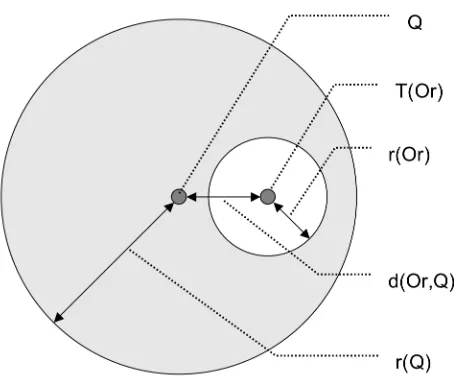
each node in the result. However, for a query Q with range r(Q), traversing the subtree

T(Or) is unnecessary. All nodes below T(Or) can be added to the results without further

computation. Since the spanning radius of a subtree is known, it is easy to determine if

the whole subtree is completely contained within the query range (Figure 7). The

(29)

Figure 7: The branch pruning method reduces the number of traversed subtrees in range queries. If the covering radius of the subtree of Or, T(Or), is within the range of the query point Q then the entire subtree T(Or) is added to the results.

01 02 03 04 05 06 07 08 09 10 11 12 13 14 15 16 17 18 19 20 21 22 range_query(N:node,Q:query_object,r(Q):range) { let Op be the parent object of node N; if N is not a leaf then {

for each Or in N do {

if |d(Op,Q)–d(Or,Op)| ≤ r(Q)+r(Or) then { compute d(Or,Q);

if d(Or,Q) + r(Or) ≤ r(Q) then add all leaves from T(Or) to result if d(Or,Q) ≤ r(Q) + r(Or) then range_query(*ptr(T(Or)),Q,r(Q)); }

} } else {

for each Oj in N do {

if |d(Op,Q)-d(Oj,Op)| ≤ r(Q) then { compute d(Oj,Q)

if d(Oj,Q) ≤ r(Q) then add oid(Oj) to the result }

} } }

(30)

01 02 03 04 05 06 07 08 09 10 11 12 13 14 15 16 17 18 19 20 21 22 23 24 25 26 27 28 29 30 31 32 33 34 35 36 k-NN_Search(T:root_node, Q:query_object,k:integer) { PR =[T,_];

for i = 1 to k do: NN[i] =[_,∞]; while PR ≠ ∅ do:

{ Next_Node = ChooseNode(PR); k-NN_NodeSearch(Next_Node,Q,k); }}

ChooseNode(PR:priority_queue): node { let dmin(T(

!

Or*)) = min{dmin(T(

!

Or))},

considering all the entries in PR; Remove entry [ptr(T(

!

Or*)),dmin(T(

!

Or*))] from PR;

return *ptr(T(

!

Or*)); }

k-NN_NodeSearch(N:node,

Q:query_object,k:integer) { let Op be the parent object of node N; if N is not a leaf then

{ ∀Or in N do:

if |d(Op,Q) − d(Or,Op)| ≤ dk + r(Op) then { Compute d(Or,Q);

if dmin(T(Or)) ≤ dk then

{ add [ptr(T(Or)),dmin(T(Or))] to PR; if dmax(T(Or)) < dk then

{ dk = NN_Update([_,dmax(T(Or))]); Remove from PR all entries for which dmin(T(Or)) > dk; }}}} else /* N is a leaf */

{ ∀Oj in N do:

if |d(Op,Q) − d(Oj,Op)| ≤ dk then {Compute d(Oj,Q);

if d(Oj,Q) ≤ dk then

{ dk =NN_Update([oid(Oj),d(Oj,Q)]); Remove from PR all entries for which dmin(T(Or)) > dk; }}}}

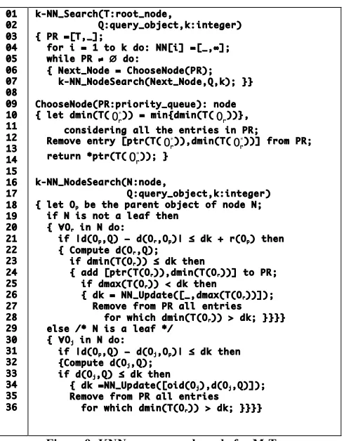
Figure 9: KNN query pseudo code for M-Tree

The k nearest neighbors (KNN) query is the other similarity query for which the

M-Tree was designed. The algorithm which performs this query over the M-Tree, shown

in Figure 9, is very much like the KNN algorithm for the R-Tree. The algorithm

traverses the tree and prunes sub-trees whose minimum distance is too large. The

minimum distance of any node in a sub-tree is:

} 0 , ) , ( max{ )) ( (

min T O = d O p "!

d _r _r

The distance of the current kth nearest neighbor provides a range that can be used

for pruning sub-trees. The minimum distance is compared with the current range and

pruning is performed if necessary. The minimum distance is also used as a heuristic when

(31)

distance allows more sub-trees to be pruned later. The reduction in distance

computations by using the parent object may be applied as in the range query.

The aggregate k nearest neighbors query is more complex than a single source

KNN query. It is a good example of the flexibility of the M-Tree for use in spatial

network algorithms. Network expansion is inefficient in solving the AKNN query and

the best known method IER still requires repeated distance computations, a slow process.

However, solving the AKNN query with the M-Tree is similar to solving a standard

single source KNN query. The major difference in the algorithms is the distance metric

used. Any distance computing between the query point and a possible result point in

KNN is replaced with an aggregate distance between all query points and a possible

result point in AKNN. For example, if the aggregate function is summation, Q is the set

of query points, and p is point currently being tested then the aggregate distance is:

!

d(p,q)

q"Q

#

The pseudo-code for the AKNN algorithm is shown in Figure 10. It should be noted that

(32)

01 02 03 04 05 06 07 08 09 10 11 12 13 14 15 16 17 18 19 20 21 22 23 24 25 26 27 28 29 30 31 32 33 34 35 36 37 Ak-NN_Search(T:root_node, Q:query_object,k:integer) { PR =[T,_];

for i = 1 to k do: NN[i] =[_,∞]; while PR ≠ ∅ do:

{ Next_Node = ChooseNode(PR); Ak-NN_NodeSearch(Next_Node,Q,k); }}

ChooseNode(PR:priority_queue): node { let dmin(T(

!

Or*)) = min{dmin(T(

!

Or))},

considering all the entries in PR; Remove entry [ptr(T(

!

Or*)),dmin(T(

!

Or*))] from PR;

return *ptr(T(

!

Or*)); }

Ak-NN_NodeSearch(N:node,

Q:query_object,k:integer) { let Op be the parent object of node N; if N is not a leaf then

{ ∀Or in N do:

if agg(|d(Op,Q) − d(Or,Op)|) ≤ agg(d(NN[k], Q)+r(Op)) then { Compute dagg (Or,Q);

if daggmin(T(Or)) ≤ dk then

{ add [ptr(T(Or)),daggmin(T(Or))] to PR; if daggmax(T(Or)) < dk then

{ dk = NN_Update([_,daggmax(T(Or))]); Remove from PR all entries

for which daggmin(T(Or)) > dk; }}}} else /* N is a leaf */

{ ∀Oj in N do:

if agg(|d(Op,Q) − d(Oj,Op)|) ≤ dk then {Compute dagg (Oj,Q);

if dagg (Oj,Q) ≤ dk then

{ dk =NN_Update([oid(Oj),d(Oj,Q)]); Remove from PR all entries

for which daggmin(T(Or)) > dk; }}}}

Figure 10: AKNN algorithm

Building the M-Tree is similar to building other index trees. The tree grows from

the bottom up and page splits increase the height of the tree. Where to insert new nodes

and how to split pages are the important differences in building the M-Tree. The

insertion algorithm chooses which sub-tree to insert the new object into based on the

increase in the covering radius. The best sub-tree is the one which has the least increase

in the covering radius. In cases where multiple sub-trees have no increase in covering

radius, the best sub-tree is the one where the new object is closest to the routing object.

Page splits are handled by partitioning the objects into two groups and promoting a node

(33)

covering radius. Similarly, the new routing objects are chosen such that the covering

radius is smallest.

Organizing the network with an M-Tree

The M-Tree is well designed to index objects in a network. The network distance

can be used to organize the M-Tree. Objects close on the network will be placed close in

the M-Tree as opposed to an R-Tree which organizes objects strictly by Euclidean

distance. There are problems, however, with indexing a road network with an M-Tree.

The major problem with using an M-Tree to index a spatial network is computing

the network distance. The distance between two objects in a network is defined as the

shortest path between those objects. Evaluating similarity queries with the M-Tree

requires repeated distance computations between objects. The M-Tree’s dependence on

distance computations makes an efficient shortest path algorithm essential to its

performance. A comparison of the different distance algorithms is important to ensure a

good balance between speed and accuracy when performing M-Tree queries.

Network Distance

Dijkstra’s Algorithm

The classic shortest path algorithm is Dijkstra’s algorithm. Dijkstra’s algorithm

computes more than just the shortest path between two nodes. It actually computes the

shortest path from the start node to every other node in the network. In many applications

computing the one-to-many shortest path is unnecessary, making Dijkstra’s algorithm

inefficient. Despite this fact many algorithms requiring shortest path computations use

Dijkstra’s algorithm. For certain graph theory applications Dijkstra’s algorithm is often

(34)

algorithm is

!

O(V+ElogV) where V represents vertices and E edges. Dijkstra’s algorithm

forms the basis for most other shortest path algorithms, and they often share its

algorithmic complexity. Alternate methods improve upon Dijkstra in absolute runtime

but have the same complexity.

A* Algorithm

The A* algorithm is a modification of Dijkstra’s algorithm which finds

one-to-one shortest paths. A* uses a heuristic to improve the search of Dijkstra’s algorithm. The

improvement of A* over Dijkstra is dependent on the heuristic. A heuristic which returns

distances close to the actual network distance will expand fewer unnecessary paths. If

the heuristic always returns a distance of zero, the A* algorithm is exactly Dijkstra’s

algorithm. At the opposite end, if the heuristic returns exactly the network distance the

A* algorithm will only traverse the exact shortest path. A heuristic for A* should always

return a distance less than the actual distance in the network in order to guarantee that a

shortest path is found. Any such heuristic is called admissible. The complexity of the A*

algorithm is

!

O(V+ElogV) the same as Dijkstra’s algorithm, because in the worst case A* is

the same as Dijkstra. However, in practice A* expands fewer nodes and thus runs in less

time than Dijkstra’s algorithm. The A* algorithm is the optimal method of determining

shortest paths between points. No other algorithm with an equivalent admissible

heuristic can find the shortest path by expanding fewer nodes.

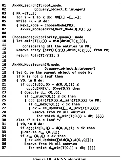
In experiments using road networks described later, the A* algorithm has

execution time which is linear with respect to distance between the two nodes of the short

(35)

properties of the M-Tree create an upper bound on the distances computed using the A*

algorithm, namely:

d ≤ r(Or) + rQ

where rQ is the query radius and r(Or) is the covering radius of routing node Or. Given

that A* computation time is linear with respect to distance a bound can be placed on the

computational cost of performing a distance computation:

!

cost(A* (v1,v2))"K(r(Or)+rQ)

v1, v2 are network vertices, K is a constant

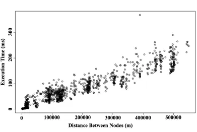
The execution time of the M-Tree when using the A* algorithm for distance

computations is much slower than comparable methods such as network expansion

(Figure 12). As a result, alternate methods of computing distance are necessary.

(36)

Figure 12: Execution time versus number of distance computations for the M-Tree with A* distance. Execution time is exponential in the number of distance computations.

Hill Climbing

The hill climbing algorithm is an alternative distance algorithm to the A*

algorithm. A heuristic is also used with the hill climbing algorithm. Instead of

expanding all necessary nodes as in the A*, the hill climbing only expands the best node

according to the heuristic. As a result, there is no guarantee that the result will be the

shortest path. The approximation of network distance may be acceptable because of

improved run time.

The increase in performance of hill climbing is significant in comparison to the

(37)

shortest path. The difficulty with overestimates is the results of a range query (RHC)

using hill climbing will always be a subset of the results (RA*) using A*.

RHC⊆ RA*

There is no good method of accounting for the nodes not included in the hill

climbing range results. It is possible to over-range the query but there is no way to

ensure the correctness of the result. In our tests the accuracy of distance computations

with the hill climbing distance is only 70%. This low accuracy reduces the usefulness of

the hill climbing algorithm. However, it is still helpful to analyze its performance when

used with the M-Tree.

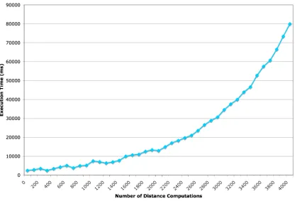
The hill climbing algorithm has performance that rivals network expansion. For

smaller range queries the M-Tree with hill climbing lags behind network expansion

(Figure 13). However, as the range increases to more than 300km the M-Tree performs

better than network expansion (Figure 14). The optimization made to the M-Tree range

query algorithm is responsible for this improvement. In fact, one can see the

optimization reducing search times to zero once the range of the query encompasses all

the objects in the network. In contrast, network expansion reaches an upper bound once

(38)

(39)

Precomputation

While hill climbing does have performance comparable to network expansion, it

is still worse than network expansion for smaller range queries. Hill climbing with the

M-Tree never shows a large improvement over network expansion for KNN queries

because there is no optimization which allows for branch pruning as done with range

queries. More importantly the hill climbing algorithm is a poor approximation for true

network distance and inaccuracies in the query results will be hard to overcome.

A much faster method of computing distance is required, one which is not a poor

approximation of network distance (like Euclidean distance). One method suggested in

the literature [4] is precomputing distance between nodes in the network.

Precomputation has the benefit that no network search is necessary to determine distance

between two points in the network. The distance will also be highly accurate because

precomputing the distances between nodes can use a highly accurate algorithm. The

computation time using precomputed distances will not be O(1) because there must be

some form of search to find the correct pair of nodes, but it should be much shorter than

traversing the network.

Unfortunately, precomputation is not actually a faster method of computing distances.

Most spatial networks are very large, encompassing millions of nodes and segments. For

a network containing Nnodes the number of distances to compute is:

!

nbdist=Nnodes(Nnodes"1)

2 =O(Nnodes

2

)

Our tests are conducted using two separate networks, one of Louisiana and one of

(40)

amount of space required to hold the distances is too large to be practical and makes

searching for distances just as slow as traversing a network, if not worse (Table 1).

Table 1: Precomputation cost using 60 nodes of a Beowulf cluster each with 50 distances / s

dataset # nodes distance computations processing time space required

LA 240,000 28 x109 3.5 months 429 GB CA 2,000,000 2 x 1012 _{20.7 years} _{29 TB}

Hill Climbing and Precomputation

Hill climbing is not quite fast enough and is not accurate. Precomputation

requires too much space to be feasible. However, combining the two may overcome both

of their deficiencies. If certain important nodes have distances precomputed then both

speed and accuracy can be improved.

Certain nodes in the network are promoted. The distance between the promoted

nodes and the points of interest indexed by the M-Tree are computed. Only the distances

to points of interest are necessary because all M-Tree queries will be over this subset of

nodes. The number of promoted nodes is much smaller than the total number of nodes.

The hill climbing algorithm is modified to check for promoted nodes along its path.

Upon reaching a promoted node, it uses the precomputed distance from that node to the

appropriate point of interest. Precomputed distances are exact. If the hill climbing

algorithm finds a promoted node then the distance estimation will be more accurate. It

will also be faster if the hill climbing algorithm is not too close to the destination node

and the number of promoted nodes is not too large (making the search slow).

The difficulty is to promote nodes which will often be reached by a hill climbing

(41)

they are heavily used, especially in longer range searches which are likely to take more

time for a hill climbing search.

There are still problems with the combination of these two methods. While better

than each individually, it is still slower than a simple Euclidean distance computation.

The distances will still be overestimates causing range queries to return too few results.

What we want is a distance algorithm on par with Euclidean distance for non-network

constrained spatial queries.

Road Network Embedding

Road Network Embedding (RNE) is a method of computing distance introduced

by Shahabi et al. [1]. Road Network Embedding uses the Linial, London, and

Robinovich (LLR) embedding technique, a kind of Lipschitz embedding [10]. An

embedding maps a point from the original space to a point in a k-dimensional vector

space.

RNE method starts by partitioning the objects in the system into subsets. For

LLR there are

!

" =O(logN) collections of subsets with each collection containing

!

"=O(logN) subsets where N is the number of points in the original space. The subsets in

each collection have

!

2i members where i is the index of the collection. The new value of

a particular location on the network is a vector with

!

"# components. Each component is

the minimum of the distance to each object in a particular subset.

The benefit of RNE is that distance in the network can be approximated by using

an LP metric in the embedded space. An Lp distance is defined as:

Lp(x,y)= xi"yi p i=1 k

#

$ %

& ' ( )

1

(42)

!

L", also called the chessboard metric, is the chosen LP metric for estimating network

distance. The chessboard metric is defined as:

!

L_"=maxi{xi#yi}

The chessboard metric is the best of the LP metrics for estimating network distance

according to Shahabi et al. [1]. Computing distances using the chessboard metric is a

simple O(1) calculation much like computing Euclidean distance. Such a

computationally simple metric is perfect for use with the M-Tree.

With RNE the new space has

!

O(log2

(N)) dimensions. Each dimension of a point in

the embedded space is actually a distance in the network. Performing RNE requires

!

O(log2

(N)) network distance computations for each point mapped to the higher dimensional

space. These distance computations must be made by a network traversal algorithm like

the A* algorithm. In order to create the complete embedding,

!

O(Nlog2

(N)) distance

computations must be performed in total. For a large network, computing that many

distances requires a substantial amount of precomputation. The space required to hold

the embedded points is also large given the high dimensionality of the new space.

Shahabi et al. [1] proposed a more limited version of RNE which does not have

the size problems of standard RNE. Truncated Road Network Embedding (tRNE) limits

the dimensionality of the embedded space. The intuition is that only the first few

dimensions of the embedding are important to the accurate calculation of network

distance. Instead of

!

"# dimensions in the embedded space, there are only pq where

1"p<<# and 1"q<<#. The cost of precomputing the entire embedding is reduced to pqN,

(43)

Using RNE does not allow computing exact network distance. The chessboard

metric in the embedded space only estimates the actual network distance. However, the

approximation using RNE is much better than the approximation using the hill climbing

algorithm. The estimate made using the chessboard metric has a maximum of

!

O(logN)

error. This approximation also has two useful properties. The first is the contractive

property:

!

dtRNE(v1,v2)"dnetwork(v1,v2)

All distances computed using RNE are less than the actual network distances, the

opposite of the hill climbing estimates. The benefit of the contractive property is that a

range query result (RRNE) using RNE to compute distance will contain all results in a

range query (RA*) using the true network distance.

RA*⊆ RRNE

The second property provides a lower bound to the error of the tRNE distance:

!

dnetwork(v1,v2)

c "dtRNE(v1,v2)"dRNE(v1,v2)"dnetwork(v1,v2)

!

c="(log(N))

The number c is called the distortion of the embedding. Given the upper and lower

bounds RNE and tRNE are assured to have a limit to the amount of error.

Cost Analysis

First is a comparison of the different distance algorithms that can be used with the

M-Tree (Table 2). We make the assumption that the network is a planar graph for

purposes of measuring complexity. The complexity of each algorithm is not an accurate

indicator of true computational time. Hill-Climbing and A* have the same complexity

(44)

comparisons of time and space complexity show that tRNE has the lowest possible time

and space complexity. Of course, the actual space required for tRNE is greater than that

required for A* and hill climbing which do not require precomputation and storage. In

comparison to A*, the only downside of tRNE is the loss of accuracy.

The preprocessing complexity of tRNE is less than that of complete

precomputation and partial precomputation (Table 3). Partial precomputation will have a

lower actual computational cost given that only a percentage of the nodes get

precomputed distances; however, it is dependent on the number of nodes in the network

and thus has the same worst case complexity as full precomputation. For determining

precomputation complexity as well as space complexity for tRNE it is assumed that a

fixed dimension is used, not one dependent on the size of the network.

Table 2: Complexity Comparison of Distance Algorithms

distance Time Space accuracy

A* O(Nlog N) O(N) 100 %

Hill climbing O(N log N) O(N) 70%

precomputation O(log2 N) O(N2) 100%

Hill Climbing + precomputation O(N log N) O(N) 70% - 100 %

tRNE O(1) O(N) > 95 %

Table 3: Pre-computation Costs for Distance Algorithms

distance pre-computation _complexity pre-computation O(N3(log N)) hill climbing +

precomputation O(N

3_{(log N))}

(45)

Experimental Results

We used two real road networks for our experiments: Louisiana and California.

The data for the road networks is US Census Bureau Tiger/LINE data. The initial data

was preprocessed to reduce the number of nodes in the network as described in the

proposed methodology. Preprocessing the data removed unnecessary nodes in the

network. In particular, nodes adjacent to only one or two other nodes are collapsed

together. These nodes increase the number of segments in the network without adding

useful information about connectivity between points of interest. Reducing the

complexity of the network improves performance of network algorithms, especially when

the network is large. The preprocessing was performed on a 72 node Beowulf cluster

because of the complexity of network reduction. Table 4 shows statistics about the data

sets and the results of graph reduction.

Table 4. Initial Statistics and Results of Graph Reduction Initial

Nodes

Post-Reduction Nodes

Reduction Factor

Points of Interest

Graph Size

Louisiana 1,200,091 137,947 88% 8,000 42 MB

California 4,931,271 624,905 87% 70,000 141 MB

The data for both road networks is held in a PostgreSQL database [8]. This

includes the network nodes and segments as well as the points of interest on the network.

For tRNE the embedded points are also contained within the database. The M-Tree index

is an external index linked into the database through external function calls. Only the

points of interest are contained within the M-Tree because range and KNN queries will

be only over this set of points.

The performance of the M-Tree was compared to that of network expansion, the

(46)

of network expansion were used for testing. The first version holds the entire network in

memory. A shared library containing the network is loaded at runtime and used to

perform the queries. The second version leaves the network in the PostgreSQL database

and uses SPI to access the data. The PostgreSQL Server Programming Interface (SPI) is

the fastest method of programmatically accessing PostgreSQL data from C code.

The actual experiments were performed on a Sun Java Workstation 1100 with a

2.2Ghz AMD64 processor and 2GB of memory. The tRNE process was performed on a

72 node Beowulf cluster. It consists of 63 slave nodes which are 2.2Ghz Intel Pentium

IV systems and 9 slave nodes which are 2.4Ghz Intel Pentium IV systems. All slave

nodes have 1 GB of memory. The master node has dual 2.2GHz Intel Xeon processors

and 2 GB of memory.

Performance of Proposed Methodology

The performance comparison is between an M-Tree using tRNE as the distance

function and both the in-memory and database versions of network expansion. It is

expected that the in-memory version of network expansion will be faster than the

database version; however, holding the entire network in-memory is impractical for many

applications.

Similar patterns of performance are seen for both range and KNN queries. Figure

16 and Figure 19 show the database version of network expansion performing much

slower than in-memory network expansion and the M-Tree. These results are to be

(47)

the in-memory version. The M-Tree index requires only index accesses to compute the

queries and is very fast as a result.

The smaller range and KNN queries show the in-memory network expansion

performing better than the M-Tree (Figure 15 and Figure 18). For ranges above 2 km the

M-Tree performs better than the in-memory network expansion. The same is true for

KNN queries where k=20. Network expansion is better for smaller queries because very

little of the network must be traversed to answer the queries. If the query can be

answered by traversing only a few segments the network expansion has to do very little

work. The M-Tree must traverse a portion of the tree to answer any query which

deprives it of the benefit of network expansion.

The density of the points of interest has an effect on these small queries, as can be

seen by the variance of the network expansion curve in Figure 17 and Figure 20. If few

points of interest are in the immediate area, more of the network must be expanded to

answer the query. The same figures show the M-Tree is not as affected by density. The

variance of the M-Tree performance is much smaller. Queries in low density areas are

where the M-Tree performs the best.

In Figure 17, one can see that the query time of network expansion plateaus at a

range of approximately 5.2x105 m. The reason is that the entire network has been

expanded and no more traversing is necessary to answer any queries. The larger the

network the greater the range necessary for the plateau to occur. Thus, for large queries

in a large network the performance benefit of the M-Tree increases even more.

The performance of the M-Tree with the more complex AKNN query is shown in

(48)

the M-Tree as both k and the number of query points vary. There is a linear relationship

between the number of query points and the query execution time. The AKNN

algorithms must perform the same computations for each query point so such a

relationship makes sense. However, these figures also show that K has a small or

negligible effect on the query execution time. The algorithm does little extra work to find

more neighbors since possible neighbors are added to a result queue as they are found.

As long as the value of k is not large, sorting the queue has only a small effect of the total

execution time of the algorithm.

Figure 22 is a comparison between the AKNN query using the M-Tree and the

IER algorithm, the best network traversal algorithm. It should be noted that the IER

algorithm actually had 4 times fewer data points from which to draw results than the

M-Tree algorithm (1000 points instead of 4000 points). However, Figure 22 still clearly

shows a vast improvement in the performance of the M-Tree over IER. The M-Tree has

execution times two orders of magnitude lower than the IER algorithm. Such a result

makes sense because the IER algorithm must perform a distance computation using

network traversal to evaluate any possible result. A large number of points in the system

requires performing many distance computations. Though this also holds for the M-Tree,

the cost of a distance computation is so low for the M-Tree that large numbers of points

(49)

Figure 15: A comparison between the M-Tree and in-memory Network Expansion (NE) for smaller range queries.

(50)

(51)

Figure 19: A KNN query comparison between the M-Tree and Network Expansion using in-memory and database networks.

(52)

(53)

Given that a database stored network is the standard, the M-Tree outperforms

network expansion tremendously. The M-Tree is at least an order of magnitude faster

than network expansion for all range query sizes and most values of k for KNN queries.

Performance for range queries larger than 3.4 km is actually two orders of magnitude

faster. Network Voronoi diagrams are at most 15 times faster than network expansion.

The M-Tree is greater than 35 times faster than network expansion at k=10 and 56 time

faster at k=20. The improvement continues to grow as k gets larger. By k=900 network

expansion takes 270 times longer to complete a query. The results for AKNN queries are

equally as impressive. The M-Tree is on average 185 times faster than IER on smaller

networks. As the network grows to include tens of thousands of nodes the performance

gap will be even larger.

Accuracy

The first experiment is a test of the accuracy of the queries performed by the

M-Tree using tRNE for distance. Because tRNE only gives an estimate of network distance,

it is important to know the quality of that estimate. Accuracy is defined as:

!

Acc= NC

NNE

where

!

NCis the number of common results between the network expansion and the

M-tree, and

!

NNE is the number of results given by the network expansion. Because

!

dtRNE"dnetwork, we expect for a range query with range

!

r_Q to have more results in the M-tree

result set than in the Network Expansion result set. The extra results will be quantified as

Improving Performance of Spatial Network Queries

ScholarWorks@UNO

ScholarWorks@UNO

Improving Performance of Spatial Network Queries

Improving Performance of Spatial Network Queries

Acknowledgements

Table of Contents

Abstract

Introduction

Background

Proposed Methodology

#

#

Experimental Results