https://doi.org/10.5194/gmd-11-4621-2018 © Author(s) 2018. This work is distributed under the Creative Commons Attribution 4.0 License.
The VOLNA-OP2 tsunami code (version 1.5)
Istvan Z. Reguly1, Daniel Giles2, Devaraj Gopinathan3, Laure Quivy4, Joakim H. Beck5, Michael B. Giles6, Serge Guillas3, and Frederic Dias2
1Faculty of Information Technology and Bionics, Pázmány Péter Catholic University, Prater u 50/a, 1088 Budapest, Hungary 2School of Mathematics and Statistics, University College Dublin, Dublin, Ireland
3Department of Statistical Science, University College London, London, UK
4Centre de Mathématiques et de Leurs Applications (CMLA), Ecole Normale Supérieure, Paris-Saclay,
Centre National de la Recherche Scientifique, Université Paris-Saclay, 94235 Cachan, France
5Computer, Electrical and Mathematical Science and Engineering Division (CEMSE), King Abdullah University
of Science and Technology (KAUST), Thuwal, 23955-6900, Saudi Arabia
6Math Institute, University of Oxford, Oxford, UK
Correspondence:Istvan Z. Reguly ([email protected]) Received: 24 January 2018 – Discussion started: 8 March 2018
Revised: 21 October 2018 – Accepted: 24 October 2018 – Published: 19 November 2018
Abstract. In this paper, we present the VOLNA-OP2 tsunami model and implementation; a finite-volume non-linear shallow-water equation (NSWE) solver built on the OP2 domain-specific language (DSL) for unstructured mesh computations. VOLNA-OP2 is unique among tsunami solvers in its support for several high-performance com-puting platforms: central processing units (CPUs), the In-tel Xeon Phi, and graphics processing units (GPUs). This is achieved in a way that the scientific code is kept separate from various parallel implementations, enabling easy main-tainability. It has already been used in production for several years; here we discuss how it can be integrated into various workflows, such as a statistical emulator. The scalability of the code is demonstrated on three supercomputers, built with classical Xeon CPUs, the Intel Xeon Phi, and NVIDIA P100 GPUs. VOLNA-OP2 shows an ability to deliver productivity as well as performance and portability to its users across a number of platforms.
1 Introduction
After the Indian Ocean tsunami of 26 December 2004, Bernard et al. (2006) emphasised that one of the greatest con-tributions of science to society is to serve it purposefully, as when providing forecasts to allow communities to respond before a disaster strikes. In the last 12 years, the
numeri-cal modelling of tsunamis has experienced great progress – see Behrens and Dias (2015). There is a variety of mathe-matical models, such as shallow-water equations (see Titov and Gonzalez (1997), Liu et al. (1998), Gailler et al. (2013), Zhang and Baptista (2008), Macías et al. (2017), and Dutykh et al. (2011)), the Boussinesq equations (see Kennedy et al. (2000) and Lynett et al. (2002)), or the Navier–Stokes equa-tions (see (Abadie et al., 2012) and Gisler et al. (2006)) and a large number of implementations, primarily for individual target computer architectures. The use cases of such models are wide ranging, and most rely on high numerical accuracy as well as high computational performance to deliver results – examples include sensitivity analysis by Goda et al. (2014), probabilistic tsunami hazard assessments by Geist and Par-sons (2006), Davies et al. (2017), and Anita et al. (2017), and more efficient and informed tsunami early warning by Yusuke et al. (2014) and Castro et al. (2015).
In Sect. 2 we discuss a number of codes currently being used in production, which as such are trusted and reliable codes, as part of a workflow. Yet, the computational perfor-mance of most of these codes is “good enough”; they were written by domain scientists and may have been tuned to one architecture or another, but, for example, GPU support is al-most non-existent. In today’s and tomorrow’s quickly chang-ing hardware landscape, however, “future-proofchang-ing” numer-ical codes is of exceptional importance for continued sci-entific delivery. Domain scientists can not be expected to keep up with architectural advances and spend a significant amount of time re-factoring code to new hardware.Whatto compute must be separated from how it is computed – in-deed in a recent paper by Lawrence et al. (2018), leaders in the weather community chart the ways forward and point to domain-specific languages (DSLs) as a potential way to ad-dress this issue.
OP2, by Mudalige et al. (2012), is such a DSL, embed-ded in C/C++ and Fortran; it has been in development since 2009. It provides an abstraction for expressing unstructured mesh computations at a high level and then provides auto-mated tools to translate scientific code written once into a range of high-performance implementations targeting mul-ticore central processing units (CPUs), graphics processing units (GPUs), and large heterogeneous supercomputers. The original VOLNA model (Dutykh et al., 2011) was already discussed and validated in detail – it was used in production for small-scale experiments and modelling but was inade-quate for targeting large-scale scenarios and statistical analy-sis; therefore it was re-implemented on top of OP2; this paper describes the process, challenges, and results from that work. As VOLNA-OP2 delivered a qualitative leap in terms of possible uses due to the high performance it can deliver on a variety of hardware architectures, its users have started in-tegrating it into a wide variety of workflows; one of the key uses is for uncertainty quantification: for the stochastic in-version problem of the 2004 Sumatra tsunami in Gopinathan et al. (2017), for developing Gaussian process emulators that help reduce the number of simulation runs in Beck and Guillas (2016) and Liu and Guillas (2017), applications of stochastic emulators to a submarine slide at the Rockall Bank in Salmanidou et al. (2017), a study of run-up behind is-lands in Stefanakis et al. (2014), the durability of oscillating wave surge converters when hit by tsunamis in O’Brien et al. (2015), tsunamis in the St. Lawrence Estuary in Poncet et al. (2010), a study of the generation and inundation phases of tsunamis in Dias et al. (2014), and others.
The time dependency in the deformation enables the tsunami to be actively generated – see Dutykh and Dias (2009). This is a step forward from the common passive mode of tsunami genesis that utilises an instantaneous rup-ture. The active mode is particularly important for tsunami-genic earthquakes with long and slow ruptures, e.g. the 2004 Sumatra–Andaman event described in Lay et al. (2005) and Gopinathan et al. (2017), and submerged landslides
in Løvholt et al. (2015), e.g. the Rockall Bank event in Salmanidou et al. (2017).
These applications present a number of challenges in in-tegration into the workflow, as well as scalable performance: the need for extracting snapshots of state variables on the full mesh, or at a number of specified locations, and capturing the maximum wave elevation or inundation – all in the context of distributed memory execution.
As the above references indicate, VOLNA-OP2 has al-ready been key in delivering scientific results in a range of scenarios, and through the collaboration of the authors, it is now capable of efficiently supporting a number of use cases, making it a versatile tool to the community; there-fore we have now publicly released it: it is freely available at https://github.com/reguly/volna (last access: 11 November 2018).
The rest of the paper is organised as follows: Sect. 2 dis-cusses related work; Sect. 3 presents the OP2 library, upon which VOLNA-OP2 is built; Sect. 4 discusses the VOLNA simulator itself, its structure, and features; Sect. 5 discusses performance and scalability results on CPUs and GPUs; and finally Sect. 6 draws conclusions.
2 Related work
Tsunamis have long been a key target for scientific simula-tions. Behrens and Dias (2015) give a detailed look at various mathematical, numerical, and implementation approaches to past and current tsunami simulations. The most common set of equations solved are the shallow-water equations, and most codes use structured and nested meshes. A popular dis-cretisation is finite differences, such codes include NOAA’s MOST (Titov and Gonzalez, 1997), COMCOT (Liu et al., 1998), and CENALT (Gailler et al., 2013). On more flexi-ble meshes many codes, such as SELFE (Zhang and Bap-tista, 2008), TsunAWI (Harig et al., 2008), ASCETE (Vater and Behrens, 2014), and Firedrake-Fluids (Jacobs and Pig-gott, 2015), use the element discretisation or the finite-volume discretisation in the cases of the VOLNA code (Du-tykh et al., 2011), GeoClaw (George and LeVeque, 2006), or HySEA (Macías et al., 2017). Another model is described by the Boussinesq equations – these equations and the solver are more complex than shallow-water solvers. Since they are primarily needed only for dispersion (see Glimsdal et al. (2013)), they are used less commonly; examples include FUNWAVE (Kennedy et al., 2000) and COULWAVE (Lynett et al., 2002). Finally, the 3-D Navier–Stokes equations pro-vide the most complete description, but they are significantly more complex than other models – examples include SAGE (Gisler et al., 2006) and the work of Abadie et al. (2012).
meshes and finite differences or finite volumes, it is unclear whether these are used in production, and they are not open source. Celeris (Tavakkol and Lynett, 2017) is a Boussinesq solver that uses finite volumes and a structured mesh – it is hand-coded for GPUs using graphics shaders, and its source code is available; however it can only use a single GPU.
As far as we are aware, only Tsunami-HySEA (Macías et al., 2017), which also uses finite volumes, uses GPU clus-ters in production – that code, however, only supports GPUs and is hand-written in CUDA. Performance reported by Cas-tro et al. (2015) on a 10 million point test case shows a sCas-trong scaling efficiency going from 1 to 12 GPUs between 88 % and 73 % (overall 12 GPUs are 5.88 faster than 1 GPU) and a 25×speed-up with 1 GPU over an unspecified (likely single core) CPU implementation. Direct comparison to VOLNA-OP2 is not possible since Tsunami-HySEA uses (nested) structured meshes, and the multi-GPU version is not open source.
3 The OP2 domain-specific language
The OP2 library (Mudalige et al., 2012) is a DSL embedded in C and Fortran that allows unstructured mesh algorithms to be expressed at a high level and provides automatic paral-lelisation and a number of other features. It provides an ab-straction that lets the domain scientist describe a mesh using a number of sets (such as quadrilaterals or vertices), connec-tions among these sets (such as edges to nodes), and data de-fined on sets (such asxandycoordinates on vertices). Once the mesh is defined, an algorithm can be implemented as a se-quence of parallel loops, each over all elements of a given set applying different “kernel functions”, accessing data either directly on the iteration set or indirectly through, at most, one level of indirection. This abstraction enables the implementa-tion of a wide range of algorithms, such as the finite-volume algorithms that VOLNA uses, but it does require that for any given parallel loop, the order of execution must not affect the end result (within machine precision) – this precludes the implementation of Gauss–Seidel iterations, for example.
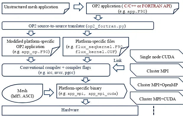
OP2 enables its users to write an application only once us-ing its API, which is then automatically parallelised to utilise multicore CPUs, GPUs, and large supercomputers through the use of MPI, OpenMP, and CUDA. This is carried out in part through a code generator that parses the parallel loop ex-pressions and generates code around the computational ker-nel to facilitate parallelism and data movement, and in part through different back-end libraries that manage data, includ-ing MPI halo exchanges, or GPU memory management, as shown in Fig. 1. For more details, see Giles et al. (2011) and Mudalige et al. (2012).
3.1 Parallelisation approaches in OP2
OP2 takes full responsibility for orchestrating parallelism and data movement – from the user perspective, the code written looks and feels like sequential C code that makes calls to an external library. To utilise clusters and supercom-puters, OP2 uses the message passing interface (MPI) to par-allelise in a distributed memory environment; once the mesh is defined by the user, OP2 automatically partitions and dis-tributes it among the available resources. It uses the stan-dard owner-compute approach with halo exchanges and over-laps computations with communications. In conjunction with MPI, OP2 uses a number of shared-memory parallelisation approaches, such as CUDA and OpenMP.
A key challenge in the finely grained parallelisation of unstructured mesh algorithms is the avoidance of race con-ditions when data are indirectly modified. For example, in a parallel loop over edges, when indirectly incrementing data on vertices, multiple edges may try to increment the same vertex, leading to race conditions. OP2 uses a colour-ing approach to resolve this; elements of the iteration set are grouped into mini-partitions, and each element within these mini-partitions is coloured, so no two elements of the same colour access the same value indirectly. Subsequently, mini-partitions are coloured as well. For CUDA, we as-sign mini-partitions of the same colour to different CUDA thread blocks, and for OpenMP to different threads. There is then a global synchronisation among different mini-partition colours. In the case of CUDA, threads processing elements within each thread block use the first level of colouring to apply increments in a safe way, with block-level synchroni-sation in between. Code generation that is suitable for auto-vectorisation by the compilers is also supported; it carries out the packing and unpacking of vector registers. The results obtained on different architectures may only differ due to differences in compiler optimisations (particularly at aggres-sive levels) and the different order in which partial results are accumulated. Previous work describes further details, accu-racy, and performance comparisons of various architectures; these are available in Mudalige et al. (2012) and Reguly et al. (2007).
3.2 Input and output
OP2 source-to-source translator (op2_fortran.py)
Conventional compiler + compiler flags (e.g. icc, nvcc, pgcc)
Hardware
Link Single node CUDA
Cluster MPI
Cluster MPI+OpenMP
Cluster MPI+CUDA Unstructured mesh application OP2 application ( C/C++ or FORTRAN API)
(e.g. app.F90)
Modified platform-specific OP2 application (e.g. app_op.F90)
Platform-specific files (e.g. flux_seqkernel.F90,
flux_kernel.CUF)
Mesh (hdf5, ASCI)
Platform-specific binary (e.g. app_mpi, app_mpi_cuda)
Figure 1.Building system with OP2.
4 The VOLNA simulator
4.1 Model, numerics, and previous validation
The finite-volume framework is the most natural numeri-cal method to solve the non-linear shallow-water equations (NSWEs), in part because of their ability to treat shocks and breaking waves. It belongs to a class of discretisation schemes that are highly efficient in the numerical solution of systems of conservation laws, which are common in com-pressible and incomcom-pressible fluid dynamics. Finite-volume methods are preferred over finite differences and often over finite elements because they intrinsically address conserva-tion issues, improving their robustness: total energy, momen-tum, and mass quantities are conserved exactly, assuming no source terms and appropriate boundary conditions. The code was validated against the classical benchmarks in the tsunami community as described below.
4.2 Numerical model
Following the needs of the target applications, the following non-dispersive NSWEs (in Cartesian coordinates) form the physical model of VOLNA:
Ht+ ∇ ·(Hv)=0, (1)
(Hv)t+ ∇ ·
Hv⊗v+g 2H
2I 2
=gH∇d. (2)
Here, d (x, t ) is the time-dependent bathymetry, v(x, t ) is the horizontal component of the depth-averaged velocity, g is the acceleration due to gravity, andH (x, t )is the total wa-ter depth. Further, I2 is the identity matrix of order 2. The
tsunami wave height or elevation of free surface η (x, t )is computed as
η (x, t )=H (x, t )−d (x, t ) , (3)
where the sum of static bathymetryds(x)and the dynamic
seabed upliftuz(x, t )constitute the dynamic bathymetry, d (x, t )=ds(x)+uz(x, t ) . (4) ds is usually sourced from bathymetry datasets pertaining
to the region of interest (for example global datasets like ETOPO1/GEBCO or regional bathymetries). The vertical componentuz(x, t )of the seabed deformation is calculated
depending on the physics of tsunami generation, e.g. via co-seismic displacement for finite fault segmentations by Gopinathan et al. (2017), submarine sliding by Salmanidou et al. (2017, 2018), etc.
In addition to the capabilities of employing active genera-tion and consequent tsunami propagagenera-tion, VOLNA also mod-els the run-up–run-down (i.e. the final inundation stage of the tsunami). These three functionalities qualify VOLNA to sim-ulate the entire tsunami life cycle. The ability of NSWEs (1)– (2) to model both propagation and run-up and run-down pro-cesses was validated in Kervella et al. (2007) and Dutykh et al. (2011), respectively. Thus, the use of a uniform model for the entire life cycle obviates many technical issues such as the coupling between the seabed deformation and the sea surface deformation and the use of nested grids.
con-strained in realistic cases. A Harten–Lax–van Leer (HLLC) numerical flux which incorporates the contact discontinuity is used to ensure that the standard conservation and consis-tency properties are satisfied: the fluxes from adjacent trian-gles that share an edge exactly cancel when summed and the numerical flux with identical state arguments reduces to the true flux of the same state. Details of the numerical imple-mentation can be found in Dutykh et al. (2011).
4.3 Validation
The original version of VOLNA was thoroughly validated against the National Tsunami Hazard Mitigation Program (NTHMP) benchmark problems (Dutykh et al., 2011). A brief look at how the new implementation, which utilises the more restrictive limiter, performs with regards to two bench-mark problems is given below. The reader is referred to the original paper (Dutykh et al., 2011) or the NTHMP website for further details on the set-up of the benchmark problems. 4.3.1 Benchmark problem 1 – solitary wave on a
simple beach
The analytical solution to the run-up of a solitary wave on a sloping beach was derived by Synolakis (1987). Thus, in this benchmark problem one compares the simulated results with the derived analytical solution.
Set-up
The beach bathymetry comprises a constant depth (d) fol-lowed by a sloping plane beach of angleβ=arccot(19.85). The initial water level is defined as a solitary wave of height ηcentred at a distanceLfrom the toe of the beach and the initial wave-particle velocity is proportional to the initial wa-ter level:
H (x,0)=ηsech2(γ (x−X1) /d) , (5)
u(x,0)= −
r
g
dH. (6)
Herex=X0=dcot(β),L=arccosh( √
20)/γ,X1=X0+ L, andγ=√3η/4d. For this benchmark problem the fol-lowing ratio must also hold:ηt /d=0.019.
Tasks
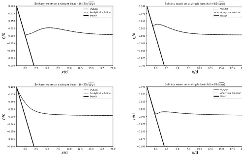
In order to verify the model, the wave run-up at various time steps (Fig. 2) and the wave height at two locations (x/d=0.25 and x/d=9.95) (Fig. 3) are compared to the analytical solution. The test was run on a node of CSD3 Wilkes2 utilising a P100 GPU.
It can be seen from the plots above that the agreement be-tween numerical results and the analytical solutions is very good. Therefore, the new implementation of the model is able to accurately simulate the run-up of the solitary wave.
4.3.2 Benchmark problem 2 – wave run-up onto a complex 3-D beach
This benchmark problem involves the comparison of lab-oratory results for a tsunami run-up onto a complex 3-D beach with simulated results. The laboratory experiment re-produces the 1993 Hokkaido–Nansei–Oki tsunami, which struck the island of Okushiri, Japan. The experiment is a 1 : 400 scale model of the bathymetry and topography around a narrow gully and the tsunami is an incident wave fed in as a boundary condition.
Set-up
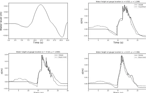
The computational and laboratory domain corresponds to a 5.49 m by 3.40 m wave tank and the bathymetry for the do-main is given for 0.014 m by 0.014 m grid cells. The incom-ing wave is incident on thex=0 m boundary and is defined for the first 22.5 s (Fig. 4a), after which it is recommended that a non-reflective boundary condition be set. At y=0, y=3.4, andx=5.5 m fully reflective boundaries are to be defined.
Tasks
The validation in the model involves comparing the temporal variation of the moving shoreline, the water height at fixed gauges, and the maximum run-up. For the basis of this brief validation, we compared the water height at three gauges in-stalled in the tank, located at (4.521, 1.196), (4.521, 1.696), and (4.521, 2.196).
It can be seen from the gauge plots in Fig. 4b–d that the first elevation wave arrives between 15 and 25 s. The overall dynamics of this elevation wave is accurately captured by the model at all the gauges, particularly the arrival time and ini-tial amplitude. Considering the results of the two benchmark tests and the full validation of the original VOLNA code, one can see that the new implementation, which implements a more restrictive limiter, still preforms satisfactorily and is consistent with the previous version. The benchmark was run on a 24-core Intel(R) Xeon(R) E5-2620 v2 CPU.
4.4 Code structure
Figure 2.Solitary wave on a simple beach – comparison between the simulated run-up and analytical solution at the shoreline (time=35, 45, 55, 65√d/g). Solid line – VOLNA; dashed line – analytical solution; thick line – beach.
Figure 3.Solitary wave on a simple beach – comparison between VOLNA and solution at different locations:(a)x/d=0.25: notice that the location becomes “dry” fort≈(67√d/g−82√d/g);(b)x/d=9.95.
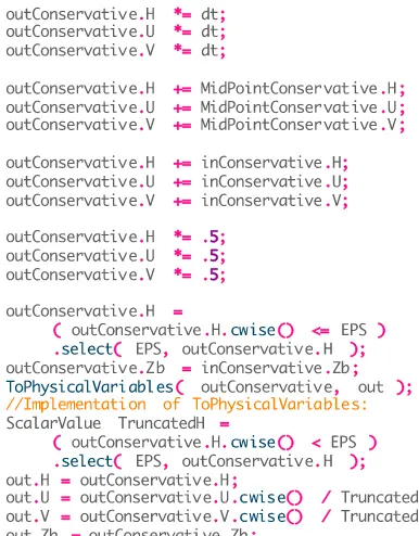
The original VOLNA source code was implemented in C++, utilising libraries such as Boost (Schling, 2011). This gives a very clear structure, abstracting data management, event handling, and low-level array operations for the higher-level algorithm – an example is shown in Fig. 5. While this
x y
x
Figure 4. (a)The incoming water level incident on thex=0 m boundary and comparison between VOLNA and laboratory results at different locations for benchmark problem 2:(b)x=4.521,y=1.196;(c)x=4.521,y=1.696;(d)x=4.521,y=2.196.
Algorithm 1Code structure of VOLNA
Initialise mesh from Gmsh file Initialise state variables
whilet < tf inaldo
Perform pre-iteration events
Third-order Runge–Kutta time stepper
Determine local gradients of state variables on each cell
Compute a local limiter on each cell
Reconstruct state variables, compute boundary conditions and determine fluxes across cell faces Compute time step
Apply fluxes and bathymetric source terms to state variables on cells
Perform post-iteration events
end while
with a mathematical formula – were implemented with func-tionality and simplicity, not performance, in mind.
To better support performance and scalability, and thus al-low for large-scale simulations, we have re-engineered the VOLNA code to use OP2 – the overall code structure is kept similar, but matters of data management and parallelism are
now entrusted to OP2. To support parallel execution we sep-arated the preprocessing step from the main body of the sim-ulation: first the mesh and simulation parameters are parsed into a HDF5 data file, which can then be read in parallel by the main simulation, which also uses HDF5’s parallel file I/O to write results to disk.
Performance-critical parts of the code, essentially any op-erations on the computational mesh, are re-implemented us-ing OP2: they are written with an element-centric approach and grouped for maximal data reuse. Calculations that were previously a sequence of operations, each calculating all par-tial results for the entire mesh, now apply only to single el-ements (such as cells or edges), and OP2 automatically ap-plies these computations to each element – this avoids the use of several temporaries and improves computational density. This process involves outlining the computational kernel to be applied at each set element (cell or edge) to a separate function and writing a call to the OP2 library – a matching code snippet is shown in Fig. 5.
Figure 5.Code snippets from the original and OP2 versions.
over which the flow will propagate. This is given through an unstructured triangular mesh. This is then transformed into a usable input to VOLNA via thevolna2hdf5code to generate compact HDF5 files. The mesh is also renumbered with the Gibbs–Poole–Stockmeyer algorithm to improve locality.
The second is the dynamic source of the tsunami. It can be an earthquake or a landslide. To describe the temporal evo-lution of seabed deformation, either a function or a series of files can be used. When a series of files is used (typically when another numerical model provides the spatio-temporal information of a complex deformation), there is a need to define the frequency of these updates in the so-called vln generic input file to VOLNA. A recent improvement has been the ability to define these series of files for a sub-region of the computational domain, and at possibly lower resolution. Per-formance is better when using a function for the seabed de-formation since I/O requirements for files can generate large overheads – VOLNA-OP2 allows for describing the initial bathymetry with an input file and then specifying relative de-formations using arbitrary code that is a function of spatial coordinates and time. Similarly, one can also define initial conditions for wave elevation and velocity.
The generic input file of VOLNA includes information about the frequency of the updates in the seabed deforma-tion, the virtual gauges in which time series of outputs will be produced, and possibly some options to output time series of outputs over the whole computational domain in order to create movies for instance. These I/O requirements obviously
affect performance: the more data to output and the slower the file system, the larger the effect.
To simulate tsunami hazard for a large number of scenar-ios is computationally expensive, so VOLNA has been re-placed in past studies by a statistical emulator, i.e. a cheap surrogate model of the simulator. To build the emulator, in-put parameters are varied in a design of experiments, and the runs are submitted with these inputs to collect input–output relationships. The output of interest could for example be the waveforms, free surface elevation, and velocity, among oth-ers. The increase in flexibility in the definition of the region over which the earthquake source of the tsunami is defined reduces the size of the series of files used as inputs: this is really helpful when a set of simulations needs to be run. Sim-ilarly, the ability to specify the relative deformation using an arbitrary code that is a function of spatial coordinates and time also reduces the computational and memory overheads when running a set of simulations.
5 Results
5.1 Running VOLNA
pro-cessing units (the Wilkes2 machine in Cambridge’s CSD3), a classical CPU architecture in the Peta-5–Skylake part of CSD3 (specifically dual-socket Intel Xeon Gold 6142 16-core Skylake CPUs), and Intel’s Xeon Phi platform in Peta-5–KNL (64-core Knights Landing-generation chips, config-ured in cache mode).
There are five key computational stages that make up 90 % of the total runtime: a stage evolving time using the third-order Runge–Kutta scheme (RK), a “gradients” stage com-puting gradients among cells, a stage that computes the fluxes across the edges of the mesh (“fluxes”), a stage that com-putes the minimum time step (“dT”), and a stage that applies the fluxes to the cell-centred state variables (“applyFluxes”). Each of these stages consist of multiple steps, but for perfor-mance analysis we study them in groups.
The RK stage is computationally fairly simple (no indi-rect accesses are made and cell-centred state variables are updated using other cell-centred state variables) and there-fore parallelism is easy to exploit, and the limiting factor to performance will be the speed at which we can move data: achieved bandwidth. Both the gradients and the fluxes stages are computationally complex and involve accessing large numbers of data indirectly through cell-to-cell and edge-to-cell mappings. The dT stage moves significant numbers of data to compute the appropriate time step for each cell, triggering an MPI halo exchange as well, and then carries out a global reduction to calculate the minimum – particu-larly over MPI this can be an expensive operation, but over-all it is limited by bandwidth. The applyFluxes stage, while computationally simple, is complex due to its indirect in-crement access patterns; per-edge values have to be added onto cell-centred values, and in parallelising this operation, OP2 needs to make sure to avoid race conditions. The per-formance of this loop is limited by the irregular access and control throughout the hardware. For an depth study of in-dividual computational loops and their performance, we refer the reader to our previous work in Reguly et al. (2007).
5.2 Tsunami demonstration case
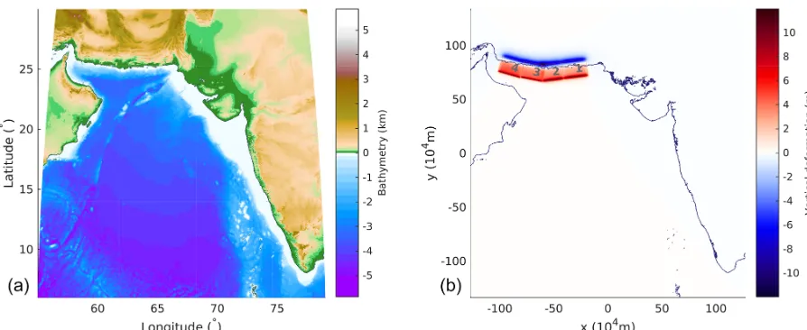
For performance and scaling analysis, we employ the Makran subduction zone as the tsunamigenic source for the numer-ical simulations. Our region of interest extends from 55 to 79◦E and from 6 to 30◦N. The bathymetry (Fig. 6a) is obtained from GEBCO (https://www.gebco.net/, last ac-cess: 11 November 2018). The region of interest is pro-jected about the centre latitude (i.e. 18◦N) to form the
rect-angular computational domain for VOLNA in Cartesian co-ordinates (Fig. 6b). This translates to a region of approxi-mately 2500 km×2700 km in area. The calculation of the sea-floor deformation or uplift (assumed instantaneous) is modelled via the Okada solution (Okada, 1992). This defor-mation is generated by the earthquake source, which is mod-elled as a four-segment finite fault model (Table 2) with a uniform slip of 30 m. The non-uniform meshes for the
sim-ulation are generated using Gmsh (Geuzaine and Remacle, 2009). A simple strategy is used to generate these meshes. Using the dimensions of the finite fault earthquake sources (l×w), an approximate source wavelength (λ0<min(l, w))
of the tsunami, and the ocean depth of the Makran trench (d0∼3 km), we calculate the time period (T) of the wave
as T =√λ0
gd0. Next, assuming that the time period of the tsunami is the same everywhere in the domain, we get for a depthdn,√λdn
n
=√λ0
d0, which in turn relates the characteristic triangle (or element) lengthhnfor depthdnashn=λk0
q dn
d0, wherek=10. At the shore (i.e.d=0), a minimum mesh size (hmin) is specified. Linear interpolation is carried out to
fur-ther smoothen the mesh gradation. A combination ofλ0and hminis used to generate a series of non-uniform meshes
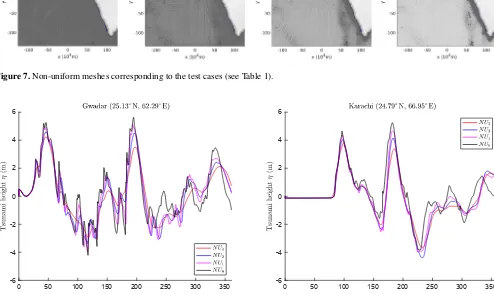
(Ta-ble 1 and Fig. 7). We also fix the triangle size as 25 km for re-gions that are deep inland. Finally, Fig. 8 shows the tsunami waveforms at two virtual gauge locations, from a run on a P100 GPU on CSD3 – the same run on the Peta-5–Skylake cluster gave results with 1.5 % (8–12 June 2015). Simulated time is 21 660 s for all mesh sizes; however, for timed runs at different scales on different platforms we restrict this to 2000 s to conserve computer time.
5.3 Performance and scaling on classical CPUs
As the most commonly used architecture, we first evalu-ate performance on classical CPUs in the Cambridge CSD3 supercomputer: dual-socket Xeon Gold 6142 CPU, with 16 cores each, supporting the AVX512 instruction set. We test a plain MPI configuration (32 processes per node), as well as a hybrid MPI+OpenMP configuration, with two MPI processes per node (one per socket), and 16 OpenMP threads each, with process and thread binding enabled.
We use OP2’s vectorised code generation capabilities, as described in Mudalige et al. (2016). The RK stage performs the same in both variants; however the fluxes and dT stages saw significant performance gains – the compiler did not au-tomatically vectorise computations; it had to be forced to do so. The applyFluxes stage could not be vectorised due to a compiler issue.
On a single node with pure MPI, running the largest mesh, 9 % of time was spent in the RK stage, achieving 182 GB s−1 throughput on average; 40 % of time was spent in the gradients stage, achieving 108 GB s−1; 25 % of time was spent in the fluxes stage, achieving 142 GB s−1; 12 % of time was spent in the dT phase, achieving 65 GB s−1; and 12 % of time was spent in the applyFluxes stage, achieving 221 GB s−1thanks to a high degree of data reuse. The maxi-mum bandwidth on this platform is 189 GB s−1as measured by STREAM Triad. The time spent in MPI communications ranged from 23 % on the smallest mesh to 10 % on the largest mesh.
prob-Figure 6. (a)Bathymetry from GEBCO’s geodetic grid is mapped onto a Cartesian grid for use in VOLNA.(b)Uplift caused by a uniform slip of 30 m in the four-segment finite fault model (given in Table 2).
Table 1.Details of the non-uniform (NU) triangular meshes.
Mesh Name Vertices Edges Triangles Sourceλ Mesh size at coast
nV nE nT λ0 hmin
NU0 53.7M 26 863 692 80 564 925 53 701 234 12.5 km 125 m
NU1 13.8M 6 931 758 20 771 822 13 840 065 25 km 250 m
NU2 3.6M 1 812 073 5 414 155 3 602 083 50 km 500 m
NU3 0.95M 485 453 1 435 017 949 565 100 km 1000 m
Table 2.Finite fault parameters of the four-segment tsunamigenic earthquake source.
Segment Length (l) Down-dip width (w) Longitude Latitude Depth Strike Dip Rake
i (km) (km) (◦) (◦) (km) (◦) (◦) (◦)
1 220 150 65.23 24.50 10 263 6 90
2 188 150 63.08 24.23 10 263 7 90
3 199 150 61.25 24.00 5 281 8 90
4 209 150 59.32 24.32 5 286 9 90
lem that the problem size per node needs to remain reason-able, otherwise MPI communications will dominate the run-time: for the NU0mesh, at 32 nodes 251 s out of 308 s
to-tal (81 %). This can be characterised by the strong scaling efficiency: when doubling the number of computational re-sources (nodes), what percentage of the ideal 2×speedup is achieved. For small node counts these values remain above a reasonable 85 %, but particularly for the smaller problems runtimes actually become worse. It is evident that on the Peta-5–Skylake cluster the interconnect used for MPI com-munications becomes a bottleneck for scaling – this overhead is significantly lower on Archer, for example; on the largest mesh at 32 nodes this overhead is only 32 %.
We have also evaluated execution with a hybrid MPI+OpenMP approach, as shown with the dashed lines in
Fig. 9a. However, on this platform it failed to outperform the pure MPI configuration.
Figure 7.Non-uniform meshes corresponding to the test cases (see Table 1).
0 50 100 150 200 250 300 350
Time (min) -6
-4 -2 0 2 4 6
0 50 100 150 200 250 300 350
Time (min) -6
-4 -2 0 2 4 6
Figure 8.Tsunami waveforms at virtual gauges located at Gwadar and Karachi.
stage with the exception of applyFluxes was vectorised – the latter was not due to compiler issues.
On a single node with pure MPI, the straightforward com-putations of the RK stage can utilise the available high bandwidth very efficiently: only 8.3 % of time spent here, achieving 194 GB s−1. The gradients stage takes 42 % of the time, achieving 82 GB s−1; the fluxes stage takes 25 % of the time and achieves 104 GB s−1; dT takes 11.4 % and achieves 46 GB s−1; and the applyFluxes stage takes 11.6 % and achieves 165 GB s−1. On the largest mesh, the Zeon Phi system is 21 % slower than a single node of the classical CPU system.
Performance when scaling to multiple nodes with pure MPI is shown in Fig. 9b: it is quite clear that scaling is worse than on the classical CPU architecture for smaller problem sizes – the Xeon Phi requires a considerably larger problem size per node to operate efficiently. Strong scaling efficiency is particularly poor on the smallest mesh, but even on the largest mesh it is only between 63 % and 92 %. Similar to the classical CPU system, the interconnect becomes a bottleneck
to scaling. Running with a hybrid MPI+OpenMP configura-tion on the Xeon Phi does improve scaling significantly, as shown in Fig. 9b – this is due to having to exchange much fewer (but larger) messages. Strong scaling efficiency on the largest problem remains above 82 %. At scale, at least on this cluster, the Xeon Phi can outperform the classical CPU sys-tem on a node-to-node basis of comparison.
5.5 Performance and scaling on P100 GPUs
1 4 16 64 256 1024 4096
1 2 4 8 16 32
Si m ul at io n ru nt im e (s )
Number of nodes
NU_3 NU_2 NU_1 NU_0
1 4 16 64 256 1024 4096
1 2 4 8 16 32
Si m ul at io n ru nt im e (s )
Number of nodes
NU_3 NU_2 NU_1 NU_0
(a) (b)
Figure 9.Performance scaling on(a)Peta-5–CPU (Intel Xeon CPU) and(b)Peta-5–KNL (Intel Xeon Phi) at different mesh sizes with pure MPI (solid) and MPI+OpenMP (dashed).
Intel’s Xeon Phi, high vector efficiency is required for good performance on the GPU.
On a single GPU, running the second-largest mesh NU1
(because NU0 does not fit in memory), 8.3 % of runtime
is spent in the RK stage, achieving 342 GB s−1; gradients takes 50 % of the time, achieving only 136 GB s−1 due to its high complexity; fluxes takes 15 %, achieving 379 GB s−1 thanks to a high degree of data reuse in indirect accesses; dT takes 4.4 % and achieves 382 GB s−1; and finally ap-plyFluxes takes 20 % of the time, achieving 204 GB s−1. In-deed, this last phase has the most irregular memory access patterns, which is commonly known to degrade performance on GPUs. Nevertheless, even a single GPU outperforms a classical CPU node by a factor of 1.5, and the Xeon Phi by 1.85.
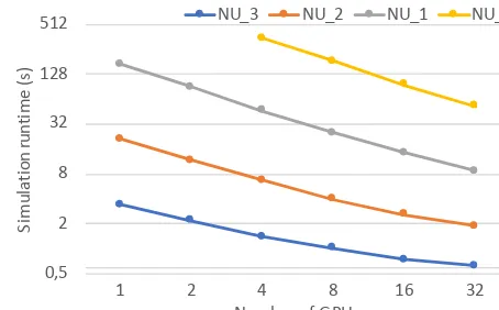
Performance when scaling to multiple GPUs is shown in Fig. 10; similar to the Xeon Phi, GPUs are also sensitive to the problem size and the overhead of MPI communications. However, given that there are four GPUs in one node, the overhead of communications is significantly lower. For the smallest problem, efficiency drops from 78 % to 58 %, and for the largest problem efficiency drops from 95 % to 89 %. Thanks to much better scaling (due to lower MPI overhead), 32 GPUs are 6.9/2.6×faster than 32 nodes of Xeon CPUs and Xeon Phi.
5.6 Running costs and power consumption
Ultimately, when one needs to decide what platform to run these simulations on, a key deciding factor aside from time to solution is cost to solution. In the analysis above, aside from discussing absolute performance metrics, we have reported speedup numbers relative to other platforms – which from a performance benchmarking perspective is not strictly fair. However, such relative performance figures combined with the cost of access do help in the decision.
Admittedly the cost of buying hardware as well as the cost of core hours or GPU hours varies significantly; therefore
0,5 2 8 32 128 512
1 2 4 8 16 32
Si m ul at io n ru nt im e (s )
Number of GPUs
NU_3 NU_2 NU_1 NU_0
Figure 10.Performance scaling on Wilkes2 (P100 GPU) at different mesh sizes.
here we do not look at specific prices. However, energy sumption is an indicator of pricing. A dual-socket CPU con-sumes up to 260 W, which is then roughly tripled when look-ing at the whole node due to memory, disks, networklook-ing, etc. In comparison, the Intel Xeon Phi CPU has a thermal design power of 215 W, roughly 750 W for the node. A P100 GPU has a TDP of 300 W, but has to be hosted in a CPU system – the more GPUs in a single machine, the better amortised this cost is: the TDP of a GPU node in Wilkes2 is around 1.8 kW (4×250 for the GPUs, plus 800 (Ithaca, New York, USA) for the rest of the system) – which averages to 450 W GPU−1. Thus in terms of power efficiency GPUs are by far the best choice for VOLNA. Nevertheless, a key benefit of VOLNA-OP2 is that it can efficiently utilise any high-performance hardware commonly available.
6 Conclusions
super-computers. By building on OP2, the science code of VOLNA itself is written only once using a high-level abstraction, cturing what to compute but not how to compute it. This ap-proach enables OP2 to take control of the data structures and parallel execution; VOLNA is then automatically translated to use sequential execution, OpenMP, or CUDA, and by link-ing with the appropriate OP2 back-end library, these are then combined with MPI. This approach also future-proofs the science code: as new architectures come along, the develop-ers of OP2 will update the back-ends and the code generators, allowing VOLNA to make use of them without further ef-fort. This kind of ease of use and portability makes VOLNA-OP2 unique among tsunami simulation codes. Through per-formance scaling and analysis of the code on traditional CPU clusters, as well as GPUs and Intel’s Xeon Phi, we have demonstrated that VOLNA-OP2 indeed delivers high perfor-mance on a variety of platforms and, depending on problem size, scales well to multiple nodes.
We have described the key features of VOLNA, the dis-cretisation of the underlying physical model (i.e. NSWE) in the finite-volume context and the third-order Runge–Kutta time stepper, as well as the input–output features that allow the integration of the simulation step into a larger workflow; initial conditions, and bathymetry in particular, can be spec-ified in a number of ways to minimise I/O requirements, and parallel output is used to write out simulation data on the full mesh or specified points.
There is still a need for even more streamlined and effi-cient workflows. For instance, we could integrate the finite fault source model for the slip with some assumptions on the rupture dynamics within VOLNA. We could also inte-grate the bathymetry-based meshing (the mesh needs to be tailored to the depth and gradients of the bathymetry to op-timally reduce computational time). Indeed, there would be even fewer exchanges of files and more efficient computa-tions, especially in the context of uncertainty quantification tasks such as emulation or inversion.
In the end, the gain in computational efficiency will allow higher-resolution modelling, such as using 2 m topography and bathymetry collected from lidar, i.e. a greater capability. It will allow greater capacity by enabling more simulations to be performed. Both of these enhancements will subsequently lead to better warnings more tailored to the actual impact on the coast as well as better urban planning since hazard maps will gain in precision geographically and probabilisti-cally due to the possibility of exploring a larger number of more realistic scenarios.
Code availability. The code is available at https://github.
com/reguly/volna/ (last access: 11 November 2018) and
https://doi.org/10.5281/zenodo.1413124 (Reguly et al., 2018). It depends on the OP2 library, which is also available at https://github.com/OP-DSL/OP2-Common (last access: 11 Novem-ber 2018), and depends on an MPI distribution, parallel HDF5, and
a partitioner, such as ParMETIS or PT-Scotch. For GPU execution, the CUDA SDK and a compatible device are required.
Author contributions. All authors contributed to the writing of the paper. IZR performed the majority of coding, with all other co-authors contributing with extensions and the numerical aspects of the code. DG and DG designed and evaluated the test cases. IZR ran the scalability studies on various supercomputers. MBG, SG, and FD provided overall supervision of the code design, evaluation, and writing.
Competing interests. The authors declare that they have no conflict of interest.
Acknowledgements. We would like to thank Endre László, for-merly of PPCU ITK, who worked on the initial port of VOLNA to OP2. István Z. Reguly was supported by the János Bólyai Research Scholarship of the Hungarian Academy of Sciences. Project no. PD 124905 has been implemented with the support provided from the National Research, Development and Innovation Fund of Hungary, financed under the PD_17 funding scheme. The authors would like to acknowledge the use of the University of Oxford Advanced Research Computing (ARC) facility in carrying out this work (https://doi.org/10.5281/zenodo.22558). Serge Guillas gratefully acknowledges support through the NERC grants PURE (Probability, Uncertainty and Risk in the Natural Environment) NE/J017434/1 and “A demonstration tsunami catastrophe risk model for the insurance industry” NE/L002752/1. Serge Guillas and Devaraj Gopinathan acknowledge support from the NERC project (NE/P016367/1) under the Global Challenges Research Fund: Building Resilience programme. Devaraj Gopinathan acknowledges support from the Royal Society, UK, and Science and Engineering Research Board (SERB), India, for the Royal Society–SERB Newton International Fellowship (NF151483). Daniel Giles acknowledges support by the Irish Research Council’s Postgraduate Scholarship Programme.
Edited by: Simone Marras
Reviewed by: two anonymous referees
References
Abadie, S. M., Harris, J. C., Grilli, S. T., and Fabre, R.: Numerical modeling of tsunami waves generated by the flank collapse of the Cumbre Vieja Volcano (La Palma, Canary Islands): Tsunami source and near field effects, J. Geophys. Res.-Oceans, 117, C05030, https://doi.org/10.1029/2011JC007646, 2012.
Acuña, M. and Aoki, T.: Real-time tsunami simulation on multi-node GPU cluster, in: ACM/IEEE conference on supercomput-ing, 14–20 November 2009, Portland, Oregon USA, 2009. Anita, G., Andrey, B., Ana, B. M., Jörn, B., Antonio, C., Gareth,
Sources and Global Applications, Rev. Geophys., 55, 1158– 1198, https://doi.org/10.1002/2017RG000579, 2017.
Barth, T. and Jespersen, D.: The design and application of upwind schemes on unstructured meshes, American Institute of Aeronau-tics and AstronauAeronau-tics, https://doi.org/10.2514/6.1989-366, 1989. Beck, J. and Guillas, S.: Sequential Design with Mutual Informa-tion for Computer Experiments (MICE): EmulaInforma-tion of a Tsunami Model, SIAM/ASA Journal on Uncertainty Quantification, 4, 739–766, https://doi.org/10.1137/140989613, 2016.
Behrens, J. and Dias, F.: New computational methods in tsunami science, Philos. T. R. Soc. A, 373, 20140382, https://doi.org/10.1098/rsta.2014.0382, 2015.
Bernard, E., Mofjeld, H., Titov, V., Synolakis, C., and González, F.: Tsunami: scientific frontiers, mitigation, forecasting and policy implications, Philos. T. R. Soc. A, 364, 1989–2007, https://doi.org/10.1098/rsta.2006.1809, 2006.
Brodtkorb, A. R., Hagen, T. R., Lie, K.-A., and Natvig, J. R.: Simulation and visualization of the Saint-Venant system using GPUs, Computing and Visualization in Science, 13, 341–353, https://doi.org/10.1007/s00791-010-0149-x, 2010.
Castro, M., González-Vida, J., Macías, J., Ortega, S., and de la Asunción, M.: Tsunami-HySEA: a GPU-based model for tsunami early warning systems, in: Proc XXIV Congress on Dif-ferential Equations and Applications, June, Cádiz, Spain, 8–12 June 2015.
Davies, G., Griffin, J., Løvholt, F., Glimsdal, S., Harbitz, C., Thio, H. K., Lorito, S., Basili, R., Selva, J., Geist, E., and Bap-tista, M. A.: A global probabilistic tsunami hazard assessment from earthquake sources, Geol. Soc. Spec. Publ., 456, 219–244, https://doi.org/10.1144/SP456.5, 2017.
Dias, F., Dutykh, D., O’Brien, L., Renzi, E., and Stefanakis, T.: On the Modelling of Tsunami Generation and Tsunami Inundation, Procedia IUTAM, 10, Mechanics for the World: Proceedings of the 23rd International Congress of Theoretical and Applied Me-chanics, ICTAM2012, 19–24 August 2012, Beijing, China, 338– 355, https://doi.org/10.1016/j.piutam.2014.01.029, 2014. Dutykh, D. and Dias, F.: Tsunami generation by dynamic
displace-ment of sea bed due to dip-slip faulting, Math. Comput. Simu-lat., 80, 837–848, https://doi.org/10.1016/j.matcom.2009.08.036, 2009.
Dutykh, D., Poncet, R., and Dias, F.: The VOLNA code for the nu-merical modeling of tsunami waves: Generation, propagation and inundation, Eur. J. Mech. B-Fluid., 30, 598–615, 2011.
Gailler, A., Hébert, H., Loevenbruck, A., and Hernandez, B.: Simulation systems for tsunami wave propagation forecast-ing within the French tsunami warnforecast-ing center, Nat. Hazards Earth Syst. Sci., 13, 2465–2482, https://doi.org/10.5194/nhess-13-2465-2013, 2013.
Geist, E. L. and Parsons, T.: Probabilistic Analysis of Tsunami Haz-ards, Nat. HazHaz-ards, 37, 277–314, https://doi.org/10.1007/s11069-005-4646-z, 2006.
George, D. L. and LeVeque, R. J.: Finite volume methods and adap-tive refinement for global tsunami propagation and local inunda-tion, Science of Tsunami Hazards, 24, 319–328, 2006.
Geuzaine, C. and Remacle, J.-F.: Gmsh: A 3-D finite ele-ment mesh generator with built-in pre- and post-processing
facilities, Int. J. Numer. Meth. Eng., 79, 1309–1331,
https://doi.org/10.1002/nme.2579, 2009.
Giles, M. B., Mudalige, G. R., Sharif, Z., Markall, G., and Kelly, P. H.: Performance analysis and optimization of the OP2 frame-work on many-core architectures, Comput. J., 55, 168–180, 2011.
Gisler, G., Weaver, R., and Gittings, M. L.: SAGE calculations of the tsunami threat from La Palma, Sci. Tsunami Hazards, 24, 288–312, 2006.
Glimsdal, S., Pedersen, G. K., Harbitz, C. B., and Løvholt, F.: Dispersion of tsunamis: does it really matter?, Nat. Hazards Earth Syst. Sci., 13, 1507–1526, https://doi.org/10.5194/nhess-13-1507-2013, 2013.
Goda, K., Mai, P. M., Yasuda, T., and Mori, N.: Sensitivity of tsunami wave profiles and inundation simulations to earthquake slip and fault geometry for the 2011 Tohoku earthquake, Earth Planets Space, 66, 105, https://doi.org/10.1186/1880-5981-66-105, 2014.
Gopinathan, D., Venugopal, M., Roy, D., Rajendran, K., Guil-las, S., and Dias, F.: Uncertainties in the 2004 Sumatra-Andaman source through nonlinear stochastic inversion of tsunami waves, P. Roy. Soc. Lond. A Mat., 473, 20170353, https://doi.org/10.1098/rspa.2017.0353, 2017.
Harig, S., Pranowo, W. S., and Behrens, J.: Tsunami simulations on several scales, Ocean Dynam., 58, 429–440, 2008.
Jacobs, C. T. and Piggott, M. D.: Firedrake-Fluids v0.1: nu-merical modelling of shallow water flows using an auto-mated solution framework, Geosci. Model Dev., 8, 533–547, https://doi.org/10.5194/gmd-8-533-2015, 2015.
Kennedy, A. B., Chen, Q., Kirby, J. T., and Dalrymple, R. A.: Boussinesq modeling of wave transformation, breaking, and runup. I: 1D, J. Waterw. Port, C., 126, 39–47, 2000.
Kervella, Y., Dutykh, D., and Dias, F.: Comparison be-tween three-dimensional linear and nonlinear tsunami gen-eration models, Theor. Comp. Fluid Dyn., 21, 245–269, https://doi.org/10.1007/s00162-007-0047-0, 2007.
Lawrence, B. N., Rezny, M., Budich, R., Bauer, P., Behrens, J., Carter, M., Deconinck, W., Ford, R., Maynard, C., Mullerworth, S., Osuna, C., Porter, A., Serradell, K., Valcke, S., Wedi, N., and Wilson, S.: Crossing the chasm: how to develop weather and climate models for next generation computers?, Geosci. Model Dev., 11, 1799–1821, https://doi.org/10.5194/gmd-11-1799-2018, 2018.
Lay, T., Kanamori, H., Ammon, C. J., Nettles, M., Ward, S. N., Aster, R. C., Beck, S. L., Bilek, S. L., Brudzinski, M. R., Butler, R., DeShon, H. R., Ekström, G., Satake, K., and Sipkin, S.: The Great Sumatra-Andaman Earthquake of 26 December 2004, Sci-ence, 308, 1127–1133, https://doi.org/10.1126/science.1112250, 2005.
Liang, W.-Y., Hsieh, T.-J., Satria, M. T., Chang, Y.-L., Fang, J.-P., Chen, C.-C., and Han, C.-C.: A GPU-Based Simulation of Tsunami Propagation and Inundation, Springer Berlin Heidel-berg, 593–603, https://doi.org/10.1007/978-3-642-03095-6_56, 2009a.
Liu, P. L., Woo, S.-B., and Cho, Y.-S.: Computer programs for tsunami propagation and inundation, Cornell University, Ithaca, New York, USA, 1998.
Liu, X. and Guillas, S.: Dimension Reduction for Gaussian Process Emulation: An Application to the Influence of Bathymetry on Tsunami Heights, SIAM/ASA Journal on Uncertainty Quantifi-cation, 5, 787–812, https://doi.org/10.1137/16M1090648, 2017. Løvholt, F., Pedersen, G., Harbitz, C. B., Glimsdal, S., and Kim, J.:
On the characteristics of landslide tsunamis, Philos. T. R. Soc. A, 373, 20140376, https://doi.org/10.1098/rsta.2014.0376, 2015. Lynett, P. J., Wu, T.-R., and Liu, P. L.-F.: Modeling wave runup with
depth-integrated equations, Coast. Eng., 46, 89–107, 2002. Macías, J., Castro, M. J., Ortega, S., Escalante, C., and
González-Vida, J. M.: Performance Benchmarking of Tsunami-HySEA Model for NTHMP’s Inundation Mapping Activities, Pure Appl. Geophys., 174, 3147–3183, https://doi.org/10.1007/s00024-017-1583-1, 2017.
Mudalige, G., Giles, M., Reguly, I., Bertolli, C., and Kelly, P.: OP2: An active library framework for solving unstructured mesh-based applications on multi-core and many-core architectures, in: In-novative Parallel Computing (InPar), San Jose, California, USA, 1–12, IEEE, 2012.
Mudalige, G. R., Reguly, I. Z., and Giles, M. B.: Auto-vectorizing a Large-scale Production Unstructured-mesh CFD Application, in: Proceedings of the 3rd Workshop on Programming Mod-els for SIMD/Vector Processing, WPMVP ’16, 12–16 March 2016, Barcelona, Spain, ACM, New York, NY, USA, 5:1–5:8, https://doi.org/10.1145/2870650.2870651, 2016.
O’Brien, L., Christodoulides, P., Renzi, E., Stefanakis, T., and Dias, F.: Will oscillating wave surge converters survive tsunamis?, Theor. Appl., 5, 160–166, 2015.
Okada, Y.: Internal deformation due to shear and tensile faults in a half-space, B. Seismol. Soc. Am., 82, 1018–1040, 1992. Poncet, R., Campbell, C., Dias, F., Locat, J., and Mosher, D.:
A Study of the Tsunami Effects of Two Landslides in the St. Lawrence Estuary, Springer Netherlands, Dordrecht, the Nether-lands, 755–764, https://doi.org/10.1007/978-90-481-3071-9_61, 2010.
Reguly, I. Z., László, E., Mudalige, G. R., and Giles, M. B.: Vec-torizing Unstructured Mesh Computations for Many-core Archi-tectures, in: Proceedings of Programming Models and Applica-tions on Multicores and Manycores, PMAM’14, 15–19 February 2014, Orlando, FL, USA, ACM, New York, NY, USA, 39:39– 39:50, https://doi.org/10.1145/2578948.2560686, 2007. Reguly, I. Z., Giles, D., Gopinathan, D., Quivy, L., Beck, J. H.,
Giles, M. B., Guillas, S., and Dias, F.: The Volna-OP2 software, version 1.5, Zenodo, https://doi.org/10.5281/zenodo.1413124, 2018.
Richards, A.: University of Oxford Advanced Research Computing, Zenodo, https://doi.org/10.5281/zenodo.22558, 2015.
Salmanidou, D. M., Guillas, S., Georgiopoulou, A., and Dias, F.: Statistical emulation of landslide-induced tsunamis at the Rock-all Bank, NE Atlantic, P. Roy. Soc. Lond. A Mat., 473, 20170026, https://doi.org/10.1098/rspa.2017.0026, 2017.
Salmanidou, D. M., Georgiopoulou, A., Guillas, S., and Dias, F.: Rheological considerations for the modelling of submarine slid-ing at Rockall Bank, NE Atlantic Ocean, Phys. Fluids, 30, 030705, https://doi.org/10.1063/1.5009552, 2018.
Satria, M. T., Huang, B., Hsieh, T.-J., Chang, Y.-L., and Liang, W.-Y.: GPU acceleration of tsunami propagation model, IEEE J. Sel. Top. Appl., 5, 1014–1023, 2012.
Schling, B.: The Boost C++ Libraries, XML Press, Amsterdam, Netherlands, 2011.
Stefanakis, T. S., Contal, E., Vayatis, N., Dias, F., and Synolakis, C. E.: Can small islands protect nearby coasts from tsunamis? An active experimental design approach, Proc. R. Soc. A, 470, 20140575, https://doi.org/10.1098/rspa.2014.0575, 2014. Synolakis, C. E.: The runup of solitary waves, J. Fluid Mech., 185,
523–545, https://doi.org/10.1017/S002211208700329X, 1987. Tavakkol, S. and Lynett, P.: Celeris: A GPU-accelerated open source
software with a Boussinesq-type wave solver for real-time in-teractive simulation and visualization, Comput. Phys. Commun., 217, 117–127, https://doi.org/10.1016/j.cpc.2017.03.002, 2017. The HDF Group: Hierarchical data format version 5, available
at: http://www.hdfgroup.org/HDF5 (last access: 11 November 2018), 2000–2010.
Titov, V. V. and Gonzalez, F. I.: Implementation and testing of the method of splitting tsunami (MOST) model, Tech. rep., NOAA Technical Memorandum ERL PMEL-112, 11 pp. UNIDATA, Washington, D.C., USA, 1997.
Vater, S. and Behrens, J.: Well-balanced inundation modeling for shallow-water flows with discontinuous Galerkin schemes, in: Finite volumes for complex applications VII-elliptic, parabolic and hyperbolic problems, Springer, Berlin, 965–973, 2014. Yusuke, O., Fumihiko, I., and Daisuke, S.: Near-field tsunami
inundation forecast using the parallel TUNAMI-N2 model: Application to the 2011 Tohoku-Oki earthquake combined with source inversions, Geophys. Res. Lett., 42, 1083–1091, https://doi.org/10.1002/2014GL062577, 2014.