* Corresponding author. E-mail address: [email protected] (B. Tokhmechi).
Journal Homepage: ijmge.ut.ac.ir
Estimation of heterogeneous reservoir parameters using Wavelet neural
network: A comparative study
Behzad Tokhmechi
a, *, Jalal Nasiri
a, Haleh Azizi
b, Minou Rabiei
b, Vamegh Rasouli
baFaculty of Mining, Petroleum and Geophysics Engineering, Shahrood University of Technology, Shahrood, Iran
bDepartment of Petroleum Engineering, University of North Dakota, United States
ABSTRACT
Static modeling of heterogeneous reservoirs remains an important challenge in petroleum engineering that requires more attentions. Ordinary Kriging (OK), sequential Gaussian simulation (SGS) or Multilayer Perceptron Neural Network (MLP) are the common methods that are utilized in modeling different type of reservoirs. However, it is well known that these methods are impractical on heterogeneous reservoirs. In this paper, Wavelet Neural Network (WNN) is introduced for modeling the heterogeneous reservoirs. In order to investigate the applicability of the WNN, two exemplar heterogeneous reservoirs were generated. The first model, represents a heterogeneous reservoir being divided into three homogeneous subzones. The second model simulates a heterogeneous reservoir composed of randomly distributed data with a wide range of variability. The applicability of such methods for porosity modeling in a heterogeneous carbonated reservoir in south-west of Iran has been investigated. The OK, MLP and WNN methods were applied to model both synthetic reservoirs. The results showed that in the second model, all three methods presented biased solutions. However, in the case of first model, the MLP resulted in biased solution, whereas the OK and WNN models presented unbiased and acceptable solutions. The results also showed that the WNN was more accurate with a lower range of error compared to the OK. In addition, it was noted that the CPU time of the WNN was approximately 15% of that of the OK, and 5% of the CPU time of the MLP. In the case of the real reservoir, all three methods resulted in unbiased solutions, because heterogeneity was less than that of both synthetic datasets. Moreover, the error of the WNN was less than that of the OK and MLP approaches, meanwhile, the WNN resulted in a lower range of error compared to the other methods. However, same as the synthetic data, the CPU time of the WNN was approximately 20% of the CPU time of the OK, and 7% of the CPU time of the MLP.
Considering the complexity associated to up-scaling the heterogeneous reservoirs and the difficulty of history matching in large blocks, which introduces large uncertainty as well, the results of this study suggests that the WNN, with a faster running time, can handle more blocks (finer grids) and offer advantages in modeling heterogeneous reservoirs.
Keywords : Heterogeneous Reservoirs, Wavelet Neural Network, Upscaling, CPU processing time, Uncertainty, Asmari
1.
Introduction
Various modeling methods have been used in reservoir characterization in the literature. Geostatistical [1, 2], intelligent [3, 4, 5], fractal [6, 7, 8], and hybrid-based modeling methods [9, 10], are some examples of many available methods. Researchers have discussed the shortcomings of some of the widely used methods when used in the simulation of heterogeneous reservoirs [11, 12].
The past studies show that the followings are the two critical factors in developing a robust estimator for modeling heterogeneous reservoirs:
Localization property: Estimators with localization properties are less influenced by heterogeneity, as they use the neighboring data for the estimation. However, those estimators that use the whole dataset on a global basis, are not able to integrate the local variabilities into the model, therefore, in heterogeneous media, the details at local scales are discarded. This suggests that in heterogeneous media, it is advisable to use the estimators that have localization properties.
CPU time: This is an important parameter to generalize the applications of an estimator to the situation where the media is composed of large datasets. The CPU time is important because
the static models should be coarse to yield reliable processing time during the history matching. In heterogeneous reservoirs, a large portion of the data variance is reduced due to the coarse block sizes used in the modeling. Although this suggests using finer size models, it introduces long processing times. Therefore, if a model offers a shorter processing time, it would be the preferred method for static modeling. The results of this work indicate that the wavelet neural network (WNN) requires less CPU time than the ordinary kriging (OK) and multilayer perceptron neural network (MLP) methods.
The literature suggests that the geostatistical estimators/simulators yield more reasonable results in heterogeneous reservoirs than other methods [11]. The use of hybrid methods with their localization property lend some promises but they suffer from long CPU times to process the data [13].
In fractal-based simulators, the idea of the cost function is to keep the fractal dimension of the data constant to ensure that the original variability of the data is maintained [14].Compared to other modeling methods, these fine-based simulators properly show the data variability of heterogeneous media. In specific, the geostatistical-based models with their cost function being based on minimizing the error, smoothen the data variability. However, the long CPU time, lack of control over the
Article History:
estimation error, and producing biased results, are the main disadvantages of multi-fractal/fractal-based simulators [15].
As already stated, the long CPU time is one of the main shortcomings of the common intelligent methods, such as the multilayer perceptron (MLP) or the radial basis function (RBF) neural networks. MLP is a global modeling method, introducing larger errors in the results comparing to common geostatistical methods in heterogeneous reservoirs [13]. RBF is a local based model requiring large datasets to generate reasonable results: this is while the reservoir datasets are generally sparse [16].
The above discussion shows the necessity of a suitable method to model complex heterogeneous reservoirs. The WNNs are the recent classes of neural networks that combine the MLP and wavelet analysis. The WNN was initially introduced to overcome the shortcomings of the MLP [17]. The WNNs are used with great success in a wide range of applications [18]. For example, it has been proven that The WNN is a valuable tool for analyzing a wide range of time-series. The WNN has already been used with success in image processing, de-noising, signal and image compression, and time-scale decomposition. The WNN is often regarded as a “microscope” in mathematics [19], and it is a powerful tool for representing nonlinearities [20].
The WNN is rarely utilized in geosciences, and especially in petroleum engineering. A few published works have shown that the WNN is a suitable method for reservoir inflow predictions [21, 22, 23]. Other researchers have suggested the WNN or wavelet for forecasting the crude oil/gas price [24, 25, 26]. The results of these studies suggest that the WNN provides better results in comparison with other common methods.
Perhaps the works conducted by Xiao-li et al. and Li-hong et al. are the first studies that compared the OK and WNN methods for grade estimation purposes [27, 28]. They reported that the WNN method, in contrary to OK, does not require any assumptions and is a less time-consuming method, while they reported that both methods presented reliable results. Niu et al. have investigated the applications of the WNN in the prediction of water content in crude oil [29]. They found that water content can be predicted with higher precisions using the WNN compared to other theoretical methods. The applications of the MLP and WNN in the estimation of the Total Oil Content (TOC) using well logs have been presented in other studies [30, 31]. These studies show that both methods yield good results at higher values of TOCs, while the MLP predicts underestimated results at the TOC values of lower than 0.4. They have also noted that the WNN gives unbiased results with higher precision than the MLP. Permeability and porosity predictions from the well logs were studied by Shokooh Saljooghi and Hezarkhani [32, 33]. Their simulation results indicated a decrease in estimation error values that depicts the ability of wavelets to enhance the function approximation capability, and better learning ability compared to the MLP neural network with different activation functions. They reported that among various mother wavelets applied as the activation functions, the Morlet function was found to be the most efficient one.
In this paper, firstly the applications of the OK and MLP, as two currently used static modeling methods, will be studied on heterogeneous reservoir datasets generated synthetically. Then, the results are compared with the proposed WNN method to compare the reliability and the CPU time of these methods.
2.
Dataset
The applications of OK, MLP, and WNN for heterogeneous
* It should be mentioned that researcher are able to control the behavior of
reservoirs modeling are studied using synthetic* and real datasets, which
are introduced in the following.
2.1.Synthetic Data Generation
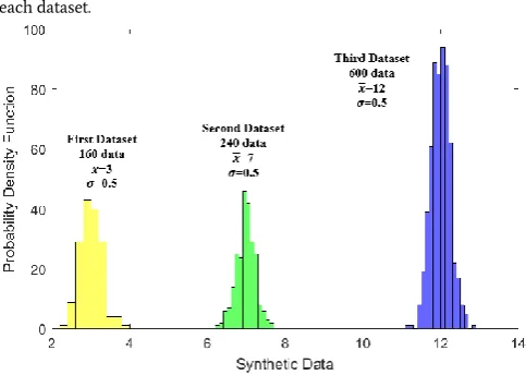
In order to generate heterogeneous data corresponding to a reservoir property, three synthetic datasets were generated having different number of data, different mean and variance (see Figure 1). The Gaussian probability density function was chosen for each dataset:
𝑓(𝑥) = 1
√2𝜋𝜎2exp(
𝑥−𝑥̅
𝜎 )
2, (1)
Where, f(x) is the probability density function, x is the property, which might be any static feature e.g. porosity or geology rock type, 𝜎 is the standard deviation of each dataset, and 𝑥̅ represents the mean of each dataset.
Figure 1. Probability density functions of three generated synthetic datasets. The reservoir was considered as a simple cube geometry with each edge comprising 10 equally spaced grids (i.e. a total of 1000 nodes) and the property assigned to each node.
In order to perform comparative studies as the objective of this work, the property was assigned to the reservoir in two different forms as show in Figure 2. In Figure 2 (left), three subzones with different sizes are considered where the distribution of data in each zone is patchy random, hence simulating a homogeneous reservoir in each zone, while the reservoir in its entirety is heterogeneous. In this case, it is expected that approaching the boundaries of each two adjacent subzones would increase the heterogeneity in data distribution. Figure 2 (right) shows the second case, where the property is assigned randomly across the entire cube, representing a homogeneous reservoir. In this situation, the values of the properties in the two adjacent nodes can exhibit either very high or low values.
2.2.Studied Reservoir
We applied the proposed methodology to an oilfield located in the southwest of Iran. More than 450 wells have been drilled in the studied area. Conventional logs include natural gamma ray, caliper, sonic, density, resistivity, and neutron ran in most of the wells. A section of the eastern part of the reservoir with seven wells was selected for this study. An Underground Counter (UGC) map of the top of the studied formation and the location of the studied wells are shown in Figure 3. The petrophysical logs as well as porosity, which was already processed and interpreted, are available in studied wells. Since the studied
reservoir is a naturally fractured carbonated formation (Asmari), there exists heterogeneity associated with the variability of porosity. The sequences of fractured zones with variable fracture density are observed along with non-fractured intervals in the Oligo-Miocene Asmari Formation [34]. Higher porosity values in upper and lower Asmari were measured, and porosity was specifically high in higher dolomitized subzones. Also, as it can be seen in Figure 3, some faults in the studied section of the reservoir are responsible for the heterogeneity and porosity of the fractures. A relatively suitable volume of data was used in this study, which enabled us to investigate the capability of the aforementioned three methods in modeling heterogeneous reservoirs.
Figure 2. Assignment of data to two synthetic cube reservoirs. A heterogeneous model with three homogeneous subzones (left) and a heterogeneous model
(right).
Figure 3. The UGC map of the oilfield and the location of studied wells.
3.
Methodologies
A brief overview of the Ordinary Kriging (OK), Multilayer Perceptron neural network (MLP) and Wavelet Neural Network (WNN) methods is presented in the following subsections. The idea is to compare the results of the OK and MLP, as the two commonly used techniques in geo-modeling in petroleum engineering applications, against the WNN proposed in this work.
3.1.Ordinary Kriging
Ordinary Kriging is a basic, linear, and unbiased average geostatistical estimator, with wide spread applications in geosciences. The procedure to conduct an OK modeling includes:
The variogram of the data is calculated and modeled through Eq. 2 [35]:
𝛾(ℎ) =(𝑍(𝑥+ℎ)−𝑍(𝑥))
2
2𝑁(ℎ) , (2)
Where, 𝛾(ℎ) is the variogram of the property for lag h, and
N(h) is the number of pair samples with distance h, and Z(x+h) and Z(x) are the values of the property in locations x+h, and x, respectively.
Extracting range, nugget, and sill values from the variogram model.
Performing a search around the point to be estimated.
Using the samples located inside the search neighborhood of a point to estimate the property of that point.
Assigning weights (Eq. 3) to the samples to reflect the spatial variability explored using the variogram model [36]:
𝑍𝑂= ∑𝑛𝑖=1𝑤𝑖𝑍𝑖. (3)
In the above equation, 𝑍𝑂 is the estimated property in point O; n represents the number of points in search sphere or ellipsoid; 𝑤𝑖 and 𝑍𝑖 are the weights and values of the property for neighboring points, respectively. The weights are determined under unbiased and minimum error variance restrictions.
3.2.Multilayer Perceptron Neural Network
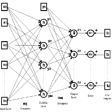
The MLP is also a widely used intelligent estimator in the field of petroleum engineering. Figure 4 illustrates a schematic architecture of the MLP.
Figure 4. A schematic architecture of the MLP.
Referring to Figure 4, the data are randomly divided into three parts: 70% for training the network and optimizing the weights of synapses, 15% for test and controlling the stop conditions, and 15% for the validation and optimization of the structure of the network (the number of layers and the number of neurons in each layer) [37].
In Figure 4, 𝑋𝑖, i=1, …, n, are input neurons, with normalized (Eqs. 4 and 5) input data being assigned to them. In the case of this study, the coordinates of the cube or reservoir nodes are the input data, which can be written as:
𝑋𝑖=
𝑋̂𝑖−𝑋𝑚𝑖𝑛
𝑋𝑚𝑎𝑥−𝑋𝑚𝑖𝑛, (4)
𝑋𝑖= 2𝑋𝑖− 1, (5)
they are transformed over the range of [-1, 1], using equation 5. The 𝑥0 and 𝑦0 are the offsets and equal to 1, giving freedom to the activation functions. The hyperbolic tangent (Eq. 6) was selected as the activation function in this work. The activation functions are shown as h and g in Figure 4. It should be mentioned that due to optimizing the weights of the offsets, the optimization of the type of activation function is not critical and was not conducted in this paper. The activation functions are defined as:
ℎ(𝑝) = 𝑔(𝑝) = 𝑡𝑔ℎ(𝑝) =𝑒𝑝−𝑒−𝑝
𝑒𝑝+𝑒−𝑝. (6)
𝑊 and 𝑈 are the synapses weight matrixes which initially are randomly generated in the range of [-0.25, 0.25], with Gaussian PDF, and need to be optimized during the process of optimization. In the following we consider all weights as 𝑊𝑖.
𝑦, 𝑍, 𝑡 and 𝑒 in Figure 4 are the output neurons of the hidden layer, output neurons of the output layer (output of network), the real output, and the error, respectively. Therefore, the structure (the number of layers and neurons) and parameters (weights) of the MLP are optimized by minimizing the error, so the developed network can be utilized for the estimation of the property at unknown points. The overall figure of the error function (cost function) when the network contains one hidden layer is developed according to equation 7 [38]:
𝑇𝑆𝑆𝐸 = ∑ ∑{𝑡𝑗− 𝑍𝑗} 2 𝐽 𝑗=1 𝑁 𝑘=1 = ∑ ∑ {𝑡𝑗− 𝑔 ( ∑ 𝑦𝑚𝑢𝑚𝑗 𝑀 𝑚=0 )} 2 𝐽 𝑗=1 𝑁 𝑘=1 = ∑ ∑ {𝑡𝑗− 𝑔 ( ∑ ℎ (∑ 𝑋𝑖𝑤𝑖𝑚 𝑛 𝑖=0 𝑢𝑚𝑗) 𝑀 𝑚=0 )} 2 𝐽 𝑗=1 𝑁 𝑘=1 (7)
In the above equation, TSSE is the total sum of the squared error for all data (train, test or validation individually), N, n, M, J are the number of data (train, test or validation individually), the number of input data, the number of neurons in hidden layer, and the number of outputs of the network, respectively.
In the case of the MLP, the architecture of neural network (the number of layers and the number of neurons in each layer) as well as the weights of synapses (𝑊 and 𝑈) were optimized using the conjugate gradient method. The conjugate gradient is an extension of the Quasi Newton, which decreases the optimization time as its main advantage [39]. The Conjugate gradient is expressed as:
𝑊𝑖+1= 𝑊𝑖− 𝜌𝑖𝑉𝑖, (8)
Where, 𝑊𝑖 is the vector of weights for synapses (𝑊 and 𝑈) in iteration i, and 𝑊𝑖+1 is the updated weights in iteration i+1. 𝑊0 are randomly generated, in the range of [-0.25, 0.25], and because of its high impact on the results, the optimization is repeated for 20 times. Here, 𝜌𝑖 is the step size in the optimization procedure that is optimized using a heuristic procedure. Also, 𝑉𝑖 is a vector, with its size similar to 𝑊, and it is calculated from partial derivative of TSSE to weights. 𝑉𝑖 is calculated as:
𝑉𝑖= 𝑙𝑖− 𝛽𝑖𝑉𝑖−1, (9)
where, 𝑙𝑖 is partial derivative of TSSE (𝛻𝑓(𝑊𝑖)) to weights, and 𝛽𝑖 is the step coefficient calculated as:
𝛽𝑖=
𝑙𝑖𝑡𝑙𝑖 𝑙𝑖−1𝑡 𝑙
𝑖−1=
‖𝑙𝑖‖2
‖𝑙𝑖−1‖2. (10)
The initial 𝑃, (𝑃0) is calculated using the initial randomly weights 𝑊0, generated as:
𝑃0= 𝑙0= 𝛻𝑇𝑆𝑆𝐸(𝑊0). (11)
Here, 𝑇𝑆𝑆𝐸(𝑊0) is the total sum of squared error of the MLP in each iteration, which is a function of weights of synapses.
It should be noted that, increasing the total sum of squared error
(TSSE) of test data in five continuous steps, is taken as the termination criterion for training the network.
3.3.Wavelet Neural Network
WNN is in fact an extension of the MLP. The two main differences between the architecture of WNN and MLP [40, 41, 42] are that:
the number of layers in the MLP should be optimized, whereas in the WNN one hidden layer is considered; and
the activation functions of WNN are mother wavelets. In fact, the activation functions in the MLP are global, but in the WNN are local with limited bands.
The above differences, offer the following two significant capabilities to the WNN [43]:
The WNN is a global modeling method. Its optimization is based on the TSSE with localization properties as its computing units (activation functions) are limited bands and are calculated in a local format [44].
The CPU time of the WNN is much less than the MLP due to the fact that the structure of the WNN is much denser than the MLP [45].
A common mother wavelet is presented in the form of [46 and 47]:
𝜓𝑎𝑗𝑏𝑗(𝑡) =
1
√𝑎𝑗𝜓 ( 𝑡−𝑏𝑗
𝑎𝑗 ) 𝑗 = 1. 2. … . 𝑘, (12)
Where, 𝜓(𝑡) is the mother wavelet at time t (in our case the location
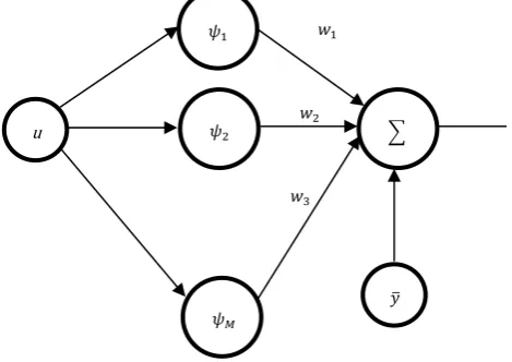
of each node), and a and b are scale and translation parameters, respectively. The structure of the WNN, with one input neuron is shown in Figure 5 [17, 41].
Figure 5. A schematic architecture of WNN with one input. 𝝍(𝒕) is the mother wavelet, and one hidden layer might be considered.
The output of the network as presented in Figure 5, is in the form of:
𝑦(𝑢) = ∑𝑀𝑖=1𝑤𝑖𝜓𝑎𝑗𝑏𝑗(𝑢) + 𝑦̅. (13)
Here, 𝑤𝑖’s are the synapses weights, and 𝑦̅ is the offset. The role of the offset is tuning the estimation, when the average is not zero [48].
In the case of WNN, as previously mentioned, only one layer was considered, and the number of neurons are optimized. Similar to the MLP, the weights of synapses as well as the dilation and translation of mother wavelets in each neuron were optimized using the conjugate gradient method. Gaussian Gradient (Eq. 14, Figure 6.a) and Mexican Hat (Eq. 15, Figure 6.b) were selected as the activation functions in this study, however, here, the results of the Gaussian Gradient are presented, because it generated better output than the Mexican Hat. Increasing the TSSE of the test data in five continuous steps was set as the termination criterion for the training.
𝜓2
𝜓𝑀
u ∑
ℎ(𝑝) = −𝑝 exp (−1
2 𝑝
2) (14)
ℎ(𝑝) = (1 − 𝑥2)exp(−𝑥
2
2) (15)
Figure 6. Two mother wavelets used as the activation functions for the WNN. Mexican Hat (left) and Gaussian Gradient (right).
4.
Results and Discussion
Results of modeling of both synthetic and real data are presented in the following.
4.1.Synthetic Data
The modeling process was carried out at all 1000 node-points of the synthetic models shown in Figure 2. In order to focus on the main objective of this study, we do not present the results of variogram modeling (in the case of OK), the optimization of weights and the training termination criterion (in the case of MLP), and also the optimization of weights-dilation-translation and the training termination criterion (in the case of WNN).
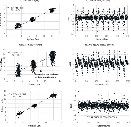
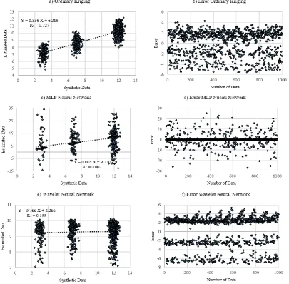
The results of three different modeling approaches and their corresponding errors for two reservoirs shown in Figure 2 are presented in Figures 7 and 8. It should be emphasized that the 3D coordinates (x, y, and z) are input values, and synthetic property, the sole output.
Figure 8. Modeling a heterogeneous exemplar reservoir (Figure 2, right) using the OK, MLP and WNN methods. The results of Figure 7, corresponds to the first reservoir, where the
heterogeneous reservoir is made of three homogeneous sub-reservoirs. In Figure 7, the WNN method appears to yield the best results with its slope of linear regression and R-squared values being close to 1. This confirms that the WNN is capable to simulate a heterogeneous reservoir which is a combination of subsets of homogeneous patches.
From Figure 6, one can say that the results of the OK are also within the acceptable range. However, the MLP method results in dispersed estimations with data scattered over a wide range and cannot be considered as a reliable model in this case. One of the shortcomings of this method is the increased variance of estimation as observed in the MLP analysis.
Another interesting outcome from this study was that the errors significantly increased at the nodes located around the borders, whereas it is close to zero in nodes at far distances from the borders. The boundary of error for the OK, MLP, and WNN are [-2.5, 2], [-6, 6] and [-1.5, 1.5], respectively. Therefore, the range of errors are 5.5, 12 and 3 for these three methods, respectively.
As explained previously, thr WNN is a global estimator, and acts as a local estimator in neighborhood of each estimation point; therefore, it can effectively consider of the impact of the nodal points at the borders of the homogeneous subzones in this example which resulted to minimal error.
The results of the analysis for the second exemplar reservoir (i.e. a heterogeneous reservoir shown in Figure 2, right) are presented in Figure 8. Here, unlike the previous example, the heterogeneity scattered in all nodes instead of being along localized regions. This creates more difficulty even for the WNN method to yield highly accurate results; therefore, it shows larger error ranges in this case comparing to those of the first example.
exemplar reservoir failed the MLP to find a reasonable trend between the data. It is to be noted that 20 runs required in order to complete the training for the MLP in an attempt to optimize the architecture of the reservoir. The results of the two examples presented above also show that, in overall, all three methods present considerable error when used to model the reservoirs with heterogeneous natures, and are not recommended for the simulations of such reservoirs.
A summary of the results of this study are presented in Table 1. As shown, the CPU times in both scenarios are almost the same. However, there is a considerable difference between the CPU times of the three methods. The CPU time for WNN is about 15% that of the OK and 5% that of the MLP. This suggests that for real reservoirs with large volume of data, due to the upscaling, the WNN is a better estimator that is faster and better suited for modeling smaller sized blocks [49]. It should be mentioned that because of the high computational cost of simulating such fine gridded models, the upscaling techniques are commonly used to reduce the resolution of the simulated models at the expense of losing accuracy.
Well 2 in Figure 3 was selected as a test, therefore, six other wells were used for training the MLP or WNN, and also variogram modeling in OK. Here also the results of variogram modeling (in the case of OK), and the optimization of weights and the training termination criterion (in the case of MLP), and also the optimization of weights-dilation-translation and the training termination criterion (in the case of WNN) are not
presented.
Table 1. Comparison between the results of various methods used to study the two exemplar reservoirs.
Heterogeneous reservoir composed of
three homogeneous patches A randomly dispersed heterogeneous reservoir
Method SSE SE Range of
error CPU Time
(second) SSE SE
Range of error
CPU Time (second)
Ordinary
Kriging 293 (unbiased) -2 5.5 61 5805
6 (biased, because of over estimation,
fig 5.a)
10 60
MLP Neural
Network 2446
441
(biased) 12 177 29028 (biased) -75 55 169
Wavelet Neural
Network 65
5
(unbiased) 3 9 12179 72 (biased) 13 8
4.2.Real Data
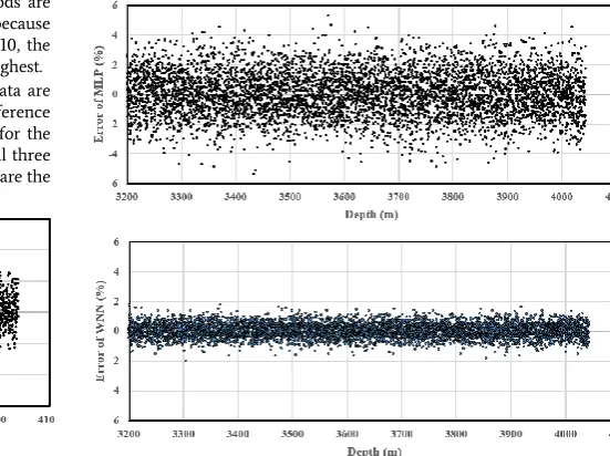
Figure 9 shows the results of estimate porosities using three methods and real porosity in well 2. Here again, the 3D coordinates are the input data and the output is porosity. It is clear in Figure 9 that the variability of estimated porosities using the MLP is higher than that of the OK and WNN.
Figure 9. Comparison between real porosity and the results of porosity estimation in well 2 in the studied oilfield. It is clear that the variability of porosity estimations for the MLP is higher than that of the OK and WNN.
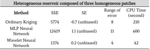
In Figure 10, the errors and their range for all three methods are mapped, clearly showing unbiased results of the estimations (because mean of errors approach to zero). Moreover, based on Figure 10, the range of error for the WNN is the lowest and for the MLP the highest. A summary of the results of this study in the case of real data are presented in Table 2. Obviously, there is a considerable difference between the CPU times of the three methods. The CPU time for the WNN is about 20% that of the OK and 7% that of the MLP. All three methods resulted unbiased estimations, while the SSE for WNN are the lowest, and the MLP is the highest.
Table 2. Comparison between the results of various methods used to modeling of Asmari reservoir.
Heterogeneous reservoir composed of three homogeneous patches
Method SSE SE Range of error CPU Time (second)
Ordinary Kriging 5774 -0.7 (unbiased) 8 210
MLP Neural
Network 12419 1.1 (unbiased) 11 600
Wavelet Neural
Network 1376 0.2 (unbiased) 4 42
5.
Conclusions
Two exemplar heterogeneous reservoirs were generated in this study to assess the application of three estimators OK, MLP, and WNN. The first one comprised three homogeneous sub-reservoirs and the second one with randomly dispersed data.
The results of modeling the first case indicated that the WNN appears to be the best estimator in terms of having the shortest CPU time, being unbiased, with a low SSE and a limited range of error. In this case, it was seen that modeling the nodes near the borders between the two adjacent sub-reservoir was the main challenge and required more attention. However, the WNN successfully models these regions due to its localized properties. The results showed that the WNN took approximately 15% of the CPU time of the OK, and 5% that of the MLP. Therefore, due to its faster running time, it can handle more blocks (finer grids) and is highly advantageous in modeling heterogeneous reservoirs.
The results of the second example showed that all three estimators were biased and yielded large error ranges.
In the case of real reservoirs, all methods resulted unbiased, acceptable solutions, while the WNN was more accurate, with a low range of error, and fast running time.
REFERENCES
[1] Almeida J.A., Use of Geostatistical Models to Improve Reservoir Description and Flow Simulation in Heterogeneous Oil Fields, Master thesis, University Technica De Lisboa, 1999, 161 pages.
[2] Hu L.Y. and Le Ravalec-Dupin M., Elements for an Integrated Geostatistical Modeling of Heterogeneous Reservoirs, Oil & Gas Science and Technology – Rev. IFP, 2004, Vol. 59 (2), pp. 141-155.
[3] Hamada G.M., and Elshafei M.A., Neural Network Prediction of Porosity and Permeability of Heterogeneous Gas Sand Reservoirs, SPE Saudi Arabia Section Technical Synposium, Al-khobar, Saudi Arabia, 2009, SPE-126042-MS, 12 pages.
[4] Cao J., Yang J., Wang Y., Wang D., and Shi Y., Extreme learning machine for reservoir parameter estimation in heterogeneous sandstone reservoir, Mathematical Problem in Engineering, 2015, Vol. 15, 10 pages.
[5] Karimi A., Moeini F., Shamsoddini-Moghadam M.J., Hosseini S.A., Mohammadi A.H., and Hemmati-Sarpardeh A., Modeling the permeability of heterogeneous oil reservoirs using a robust method, Geosciences Journal, 2016, Vol. 20, pp. 259-271.
[6] Hewett T.A., Fractal distribution of reservoir heterogeneity and their influence of fluid transport, 61st Ann. Tech. Conf. New Orleans, Louisiana, 1986, SPE 15385.
[7] Hewett T.A., Modelling Reservoir Heterogeneity with Fractals, Quantitative Geology and Geostatistics, 1993, Vol. 5, pp. 455-466.
[8] Al-Zainaldin S. Glover PWJ. and Lorinczi P., Synthetic Fractal Modelling of Heterogeneous and Anisotropic Reservoirs for use in Simulation Studies: Implications on their Hydrocarbon Recovery Prediction, Transport in Porous Media, 2017, Vol. 116 (1), pp. 181-212. [9] Michael H.A., Li H., Boucher A., Sun T., Caers J., and
Gorelick S.M., Combining geologic-process models and geostatistics for conditional simulation of 3-D subsurface heterogeneity, Water Resources Research, 2010, Vol. 46, 20 pages.
[10] Shiri Y. Tokhmechi B. Zarei Z. Koneshloo M., Self-Affine and ARX-Models Zonation of Well Logging Data, Physica A: Statistical Mechanics and its Application, 2012, Vol. 391 (21), pp. 5208-5214.
[11] Deutsch C.V., What in the Reservoir is Geostatistics Good For? Journal of Canadian Petroleum Technology, 2006, Vol. 45, pp. 201-225.
[12] Rasouli V. Tokhmechi B., Difficulties in using geostatistical models in reservoir simulation, 2010, SPE 126191, Egypt. [13] Tokhmechi B. Rasouli V. Azizi H. Rabiei M., Hybrid
Clustering-estimation for Characterization Thin Bed Heterogeneous Reservoirs, Carbonates and Evaporites, 2018, DOI: 10.1007/s13146-018-0435-0, pp. 1-13. [14] Tokhmechi B., The use of the fractal method for
simulation of the topographic surfaces, The Journal of Amir Kabir, 2004Vol. 59.D, pp. 41 – 52.
[15] Majumdar A. and Tien CL., Fractal characterization and simulation of rough surfaces, Wear, 1990, Vol 136, Issue 2, pp. 313-327.
[16] Lefteri H. Tsoukalas and Robert E. Uhrig, Fuzzy and Neural Approaches in Engineering, New York: John Wiley & Sons, Inc. 1997.
[17] Zhang Q. and Beveniste A., Wavelet networks, IEEE Transactions on Neural Networks, 1992, Vol. 3, pp. 889– 898.
[18] Alexandridis A.K. and Zapranis A.D., Wavelet neural networks: A practical guide, Neural Networks, 2013, Vol. 42, pp. 1-27.
[19] Cao L. Hong Y. Fang H. and He G., Predicting chaotic time series with wavelet networks, Physica D, 1995, Vol. 85, pp. 225–238.
[20]Fang Y. and Chow T.W.S., Wavelets based neural network for function approximation, Lecture notes in computer science, 2006, Vol. 3971, pp. 80–85.
[21] Okkan U., Wavelet neural network model for reservoir inflow prediction, Sceintia Iranica A., 2012, Vol 19 (6), pp. 1445-1455.
[22]Fengqi h. and Lijuan S., Wavelet Neural Network in the Design and Application of Hydrological Forecast, International Conference on Intelligent Transportation, Big Data and Smart City, Halong Bay, Vietnam, 2015, 12 pages.
[24]Alexandridis A. and Livanis E., Forecasting Crude Oil Prices Using Wavelet Neural Networks, 5th Student Conference of Management Science and Technology, Athens, Greece, 2008, 8 pages.
[25]Yu L. Pang Y. Wei X. and Xu S., Forecasting crude oil spot price by wavelet neural networks using OECD petroleum inventory levels, New Mathematics and Natural Computation, 2011, Vol 7 (2), pp. 281-297.
[26]Jin J. and Kim J., Forecasting Natural Gas Prices Using Wavelets, Time Series, and Artificial Neural Networks, Plos One, 2015, 10 pages.
[27]Xiao-li L. Yu-ling X. Li-hong L. and Qin-jin G., A nonlinear grade estimation method based on Wavelet Neural Network, 4th International Conference on Bio-Inspired Computing, Beijing, China, 2009, 8 pages.
[28]Li-hong L. Xu X.Y. Liu Y.F. and Xiao-li L., An Uncertainty Oriented Grade Estimation Method Based on Fuzzy Wavelet Neural Network, 2nd International Workshop on Intelligent Systems and Applications, Wuhan, China, 2010, 8 pages.
[29]Niu H. Liu C. Wang J. and Sun X., Application of Wavelet Neural Network to Prediction of Water Content in Crude Oil, Advances in Neural Network Research and
Applications, 2010, Vol. 67, pp. 21-27.
[30]Nasiri J. Tokhmechi B. Rezaee M.R., TOC estimation using wavelet neural network from well log data, The First International Conference of Oil, Gas, Petrochemical and Power Plant, Tehran, Iran, 2012, 10 pages.
[31] Nasiri J., TOC estimation from logs using wavelet neural network, case study: Kockatea shale, Perth sedimentary basin, Western Australia, MSc thesis, Shahrood University of Technology, 2013, 116 pages.
[32]Shokooh Saljooghi B. and Hezarkhani A., Comparison of WAVENET and ANN for prediction the porosity obtained from well log data, Journal of Petroleum Science and Engineering, 2014, Vol. 123, pp. 172-182.
[33]Shokooh Saljooghi B. and Hezarkhani A., A new approach to improve permeability prediction of petroleum reservoirs using neural network adaptive wavelet (wavenet), Journal of Petroleum Science and Engineering, 2015, Vol. 133, pp. 851-861.
[34]Alavi M., Regional stratigraphy of the Zagros fold-thrust belt of Iran and its proforeland evolution, American Journal of Science, 2004, Vol. 304, pp. 1-20.
[35]Isaaks E.H. and Srivastava R.M., An introduction to applied geostatistics, Oxford University Press (New York), 1989, 561 pp.
[36]Armstrong M. (Ed.), Basic linear geostatistics, Springer-Verlag (Berlin), 1998, 256 pp.
[37]Boughrara H. Chtourou M. Amar C.B. and Chen L., MLP neural network using modified constructive training algorithm: Application to face recognition, Image Processing, Application and System Conference (IPAS), Sousse, Tunisia, 2014, 8 pages.
[38]Bishop, C.M., Neural Networks for Pattern Recognition, Oxford University Press, 1997, 508 pages.
[39]Fletcher, R., Practical Methods of Optimization, Volume 1: Unconstrained Optimization, John Wiley & Sons, 1980, 120 pages.
[40]Bakshi V. Stephanopoulos R. and Bhavik G., Wavelets as basic functions for localized learning in multi-resolution hierarchy, IEEE, 1992, Vol. 2, pp. 140-145.
[41] Veitch D., Wavelet Neural Networks Data Analysis, Networks and Nonlinear Dynamics, MSc. Thesis, University of York, 2005.
[42]Chen Y., Yang B., and Dong J., Time-series prediction using a local linear waveletneural network, Neurocomputing, 2006, Vol. 69, pp. 449–465.
[43]Zhang X.S., Neural Networks in Optimization, Springer, 2000, pages 61-103.
[44]Avci E., An expert system based on wavelet neural network-adaptive 115 normentropy for scale invariant texture classification, Expert Systems with Applications, 2007, Vol. 32, pp. 919–926.
[45]Zhang Z., Learning algorithm of wavelet network based on sampling theory, Neurocomputing, 2007, Vol. 71, pp. 244– 269.
[46]Daubechies, I., The wavelet transform, time frequency localization and signal analysis, IEEE Trans. Inform. Theory, 1990a, Vol. 39, pp. 961-1005.
[47]Daubechies, I., Ten lectures on wavelets, 1990b, 268 Pages. [48]Cheng J. L., Wavelet Neural networks with a hybrid
learning approach, Journal of Information Science and Engineering, 2006, Vol. 22, pp. 1367-1387.