Wind reconstruction algorithm for Viking Lander 1

(1)

Geosci. Instrum. Method. Data Syst., 6, 217–229, 2017 https://doi.org/10.5194/gi-6-217-2017

Wind reconstruction algorithm for Viking Lander 1

Tuomas Kynkäänniemi1_{, Osku Kemppinen}2,a_{, Ari-Matti Harri}2_{, and Walter Schmidt}2 1_{School of Science, Aalto University, Espoo, Finland}

2_{Earth Observation, Finnish Meteorological Institute, Helsinki, Finland}

a_{currently at: Department of Physics, Kansas State University, Manhattan, Kansas, USA} Correspondence to:Tuomas Kynkäänniemi ([email protected])

Received: 8 December 2016 – Discussion started: 22 February 2017 Revised: 18 May 2017 – Accepted: 19 May 2017 – Published: 22 June 2017

Abstract.The wind measurement sensors of Viking Lander 1 (VL1) were only fully operational for the first 45 sols of the mission. We have developed an algorithm for reconstructing the wind measurement data after the wind measurement sen-sor failures. The algorithm for wind reconstruction enables the processing of wind data during the complete VL1 mis-sion. The heater element of the quadrant sensor, which pro-vided auxiliary measurement for wind direction, failed dur-ing the 45th sol of the VL1 mission. Additionally, one of the wind sensors of VL1 broke down during sol 378. Regardless of the failures, it was still possible to reconstruct the wind measurement data, because the failed components of the sen-sors did not prevent the determination of the wind direction and speed, as some of the components of the wind measure-ment setup remained intact for the complete mission.

This article concentrates on presenting the wind recon-struction algorithm and methods for validating the operation of the algorithm. The algorithm enables the reconstruction of wind measurements for the complete VL1 mission. The amount of available sols is extended from 350 to 2245 sols.

1 Introduction

The primary goal of the Viking mission was to investigate the current or past existence of life on Mars. The Viking Lander’s payload (Soffen, 1977) consisted of instruments de-signed for meteorological experiments (Chamberlain et al., 1976), for seismological measurements and for experiments on the composition of the atmosphere.

Viking Lander 1 (VL1) landed on Mars on 20 July 1976. The location of the landing spot was a low plain area named

Chryse Planitia, which has a slope rising from south to west. The landing coordinates of VL1 were 22◦N, 48◦W.

VL1 operated for 2245 Martian sols, which is much longer than was expected (Soffen, 1977). Thus the data set produced is significant in size. The VL1 data set enables the study of various meteorological phenomena ranging from diurnal to seasonal timescales using measurements of temperature, pressure and wind direction.

The Finnish Meteorological Institute (FMI) has devel-oped a set of tools that enable processing the Viking Lan-der meteorological data beyond previously publicly avail-able data in the National Aeronautics and Space Adminis-tration’s (NASA) Planetary Data System (PDS; Kemppinen et al., 2013). Currently NASA’s PDS contains wind measure-ment data only from 350 sols. The FMI tools make it possible to process data from the full 2245 sols instead, over a sixfold increase.

(2)

not fully functional due to hardware issues. It is still possi-ble to use the MSL wind sensor to retrieve wind speeds and accurate wind directions if the wind comes from the hemi-sphere in front of the rover (Newman et al., 2016). Thus, the VL1 wind measurement data set remains the longest data set of wind measurements from the surface of Mars at least for the coming years.

This article focuses on the reconstruction of the VL1 wind measurements. Section 2 provides an overview of the VL1 wind sensors and their malfunctions. The wind reconstruc-tion algorithm is defined in Sect. 3, and the validareconstruc-tion meth-ods for the algorithm are presented in Sect. 4. The recon-structed data from the VL1 wind measurements are presented in Sect. 5.

The significance of this work lies in the fact that other mis-sions on the surface of Mars have not yet succeeded in mea-suring a data set equal to the size of that of VL1. Even though the VL1 landed on Mars 40 years ago, not all the data from the VL1 wind instruments have been analyzed and published due to various complications that are described below.

2 Wind measurement setup and sensor malfunctions 2.1 Wind sensors

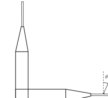
The Viking Lander wind measurement setup consisted of two hot-film wind sensors and a quadrant sensor (Chamberlain et al., 1976). The hot-film wind sensors were designed to de-termine the wind velocity component normal to each of the sensors, and the quadrant sensor was designed to provide in-formation about the wind direction and therefore solve the fourfold ambiguity of the normal components (Chamberlain et al., 1976).

The wind sensor design is presented in Fig. 1. The hot-film wind sensors were mounted at a 90◦angle with respect to each other, and the temperature of the films was main-tained at 100◦_{C above the ambient gas temperature. The} sen-sor convective heat transfer can be represented by the Nusselt number:

Nu= Q

π LκF1T

, (1)

whereQ is the power convected to the fluid,Lis the ele-ment length, κF is the gas thermal conductivity (at the gas

film temperature) and 1T is the element overheating tem-perature. The wind velocity normal to each hot-film sensor could be determined from the power required to maintain the overheating temperature against heat loss due to radia-tion and conducradia-tion. Assuming the wind velocity is a vector v from directionθ, as presented in Fig. 1, the perpendicular wind speed componentsvxandvycan be determined by

Figure 1.Wind sensor design. The hot films were mounted at the end of two separate holders, which were set perpendicular to each other (Davey et al., 1973).

vy= |v|sin(θ ), (2)

vx= |v|cos(θ ). (3)

There exists a fourfold ambiguity in the wind velocity measured by the two wind sensors. The ambiguity is caused by the wind sensors only measuring the wind velocity com-ponent normal to the sensor, and it is resolved using the quad-rant sensor (Davey et al., 1973; Sutton et al., 1978).

2.2 Quadrant sensor

The quadrant sensor was designed to provide a secondary measurement to solve the ambiguity in the wind direction. The design of the sensor is presented in Fig. 2. The operating principle of the sensor is based on locating the thermal wake of a heated vertical cylinder. The location of the wake is de-termined from the temperature distribution about the cylinder using four chromel–constantan thermocouples (TCs). These thermocouples were connected in series, and each pair mea-sures the temperature difference across the sensor due to the thermal wake (Davey et al., 1973; Sutton et al., 1978). 2.3 SANMET

(3)

T. Kynkäänniemi et al.: Wind reconstruction algorithm for Viking Lander 1 219

Figure 2.Quadrant sensor design (Hess et al., 1977).

SANMET output under the DATA6 header. The algorithm additionally requires the wind directionsθ and the Nusselt numbersNu₁andNu₂of the wind sensors during sols 1–45. 2.4 VL1 sensor malfunctions

The heater element of the VL1 quadrant sensor was thought to be damaged during the 45th sol (Murphy et al., 1990; Hess et al., 1977). During sol 46 there exists a sudden change in the behavior of the voltage values of the thermocouple pairs QS1 and QS2, which is shown in Fig. 3. When the quadrant sensor was functioning in the intended way, the voltage val-ues of QS1 and QS2 varied within ±5.0 mV, but after the failure of the heater element the variation range of the volt-ages changed to approximately±0.5 mV.

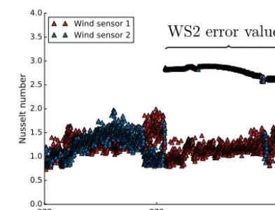
After the failure of the quadrant sensor’s heater element, the SANMET process for determining the wind direction was no longer fully reliable. It is assumed that both of the quadrant sensor thermocouples remained functional for the whole VL1 mission. Therefore the instrument can be used whenever the radiance of the Sun is strong enough to heat the quadrant sensor’s heater element to a temperature where the bias-corrected thermocouples’ signals exceeded 0.05 mV. In addition to the failure of the quadrant sensor’s heater element, one of the two hot-film wind sensors of VL1 broke down during sols 377–378. The decay of the VL1 wind sen-sor 2 is illustrated in Fig. 4 by presenting the unbinned values of the Nusselt number measured by both of the wind sensors.

45 46 47 48 49

Sol

4 2 0 2 4

Voltage (mV)

QS1 QS2

Figure 3.Failure of the heater element of VL1’s quadrant sensor during sol 46.

377 378 379

Sol

0.0 0.5 1.0 1.5 2.0 2.5 3.0 3.5 4.0

Nusselt number

Wind sensor 1

Wind sensor 2

WS2 error values

1

Figure 4.The decay of the VL1’s wind sensor 2 (WS2) during sols 377–378.

At the turn of sols 377 and 378, the dynamic of the wind sen-sor 2 changed so that the sensen-sor obtains almost constant Nus-selt number of slightly less than 3.0. At the end of sol 378’s measurements the wind sensor 2 resumed nominal function for a very short period of time, after which the behavior of the sensor returned to the failure state permanently.

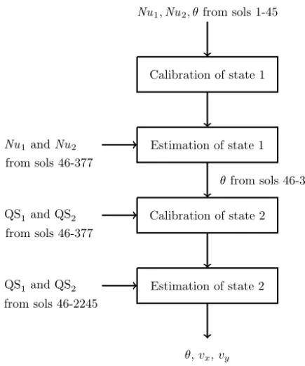
3 Wind reconstruction algorithm

(4)

Figure 5. Schema of the complete processing chain of the wind reconstruction algorithm.Nu₁andNu₂are the Nusselt numbers of wind sensors 1 and 2, QS₁and QS₂are the voltage values of the thermocouple pairs,θis the wind direction, andvxandvyare the

wind speed normal components.

and then an estimation phase, where the wind directionθ is estimated.

In the first stage the wind directions of the fully functional quadrant sensor are used to calibrate the two hot-film sen-sors’ Nusselt numbers. The method of calibrating the Nusselt numbers with the correct wind direction data from sols 1–45 is presented in Sect. 3.2. The Nusselt numbers of the two hot-film wind sensors are then used for determining the wind di-rection during sols 46–377. The reconstruction of wind direc-tion after sol 376 is unfortunately impossible using the cali-brated Nusselt numbers, as one of the two sensors failed dur-ing sol 378. Therefore in the second stage, the reconstructed wind directions from sols 46–377 are required for calibrating the weak voltage signals of the quadrant sensor, to enable the estimation of wind direction after sol 377 with the quadrant sensor.

In the second stage the reconstructed wind directions, de-termined using the Nusselt numbers of wind sensors, are used to calibrate the quadrant sensor voltages. The quadrant sen-sor thermocouple pairs continued working nominally after the heater element failure. The voltages observed by the ther-mocouples are weaker and contain more noise, but they have the same dynamic as during sols 1–45, when the heater ele-ment was intact. Section 3.5 presents a method for

calibrat-ing the quadrant sensor voltages with the reconstructed wind directions from sols 46–377.

After calibrating the voltages of the quadrant sensor, the wind directions can be solved for sol 377 and beyond. With the reconstructed wind direction and one stream of intact wind component data the wind speeds can be solved for sol 377 and onwards. The complete VL1 mission was recon-structed using the calibrated quadrant sensor signals, which were calibrated using the Nusselt number wind direction es-timates from stage one.

3.2 Calibration of the wind sensors

The wind direction can be obtained from the Nusselt num-bers. This is because the Nusselt numbers are dependent on the wind components normal to the hot-film sensors. The first stage of the wind reconstruction algorithm relies on the as-sumption that the wind sensors get similar values for Nusselt numbers during the period of interest to those during sols 1–45. The values of Nusselt numbers for both wind sensors were examined from arbitrary sols from the sol interval 46– 377 of the VL1 mission. The results from this spot check were encouraging as the Nusselt numbers of the wind sensors remained the same order of magnitude during the examined sols. The method of using the Nusselt numbers for estimating the wind direction was first studied by Murphy et al. (1990). The method used here is similar to method used in Murphy et al. (1990), but it contains less subjectivity in the process as the wind directions are not reconstructed mechanically by hand.

The reconstruction algorithm begins by computing first the calibration functionsFi, for different wind velocity classes,

from the Nusselt numbers Nu₁ and Nu₂ measured by the wind sensors. The calibration functions Fi are defined the

same way as in Murphy et al. (1990):

F =(Nu√1−Nu2)

Nu1Nu2 . (4)

After the values forF were calculated by Eq. (4), they were binned into 1◦_{-sized bins. Then, 12th-order} polynomi-als were fitted to the binned values calculated with Eq. (4). The polynomials with degreen=1, . . .,15 were considered. For 12th-order polynomials, the mean absolute difference of the reconstructed angle and the SANMET-provided “correct” angle from sols 1–45 was the smallest.

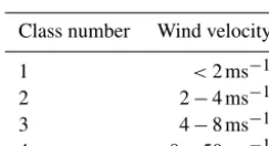
Because the Nusselt numbers depend on the wind ve-locity, the velocities were divided into four different veloc-ity classes. For each velocveloc-ity class the calibration function was obtained using the method described earlier. Table 1 presents the different velocity classes for which the calibra-tion funccalibra-tionsFi were determined. Wind velocities greater

(5)

0 40 80 120 160 200 240 280 320 360

Wind direction (

◦

)

0.4 0.3 0.2 0.1 0.0 0.1 0.2

F

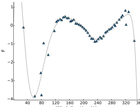
Figure 6.Calibration functionF₁for velocity class 1.

Table 1.The velocity classes of the wind reconstruction algorithm.

Class number Wind velocity 1 <2 ms−1

2 2−4 ms−1

3 4−8 ms−1

4 8−50 ms−1

from these velocities to produce good statistics, and the ve-locities were ignored.

The calibration functionsFi for each wind class are

plot-ted in Figs. 6, 7, 8 and 9 with gray-colored curves. Although there exists a slight overfitting effect in the calibration func-tions in Figs. 6, 8 and 7, the calibration funcfunc-tions can distin-guish the wind directions from different F values as the data are distributed uniformly to the full angle interval. For the calibration in Fig. 9 the data are not distributed evenly to the complete angle interval, which reduces the accuracy of the wind direction estimates.

The data for the calibration functions in Figs. 6, 8, 7 and 9 were obtained from the first 45 sols, when the quadrant sen-sor was still fully functional, and it consisted of 53 229 mea-surement samples. Most of the samples were from conditions where the wind velocity was less than 8.0 ms−1.

To reconstruct the wind directions of a complete sol, the algorithm calculates for each measurement sample the value of functionF using Eq. (4) and determines the velocity class of the sample. With the calculated F value, the roots θi of

12th-order polynomial were calculated by solving

12 X

i₌0

aiθi−Fsample=0. (5)

The coefficientsai of the polynomial were obtained from

the calibration function fit. The rootsθi of Eq. (5) were used

0 40 80 120 160 200 240 280 320 360

Wind direction (

◦

)

0.8 0.6 0.4 0.2 0.0 0.2 0.4 0.6 0.8

F

Figure 7.Calibration functionF₃for velocity class 3.

0 40 80 120 160 200 240 280 320 360

Wind direction (

◦

)

0.6 0.4 0.2 0.0 0.2 0.4

F

Figure 8.Calibration functionF₂for velocity class 2.

as candidate angles for wind direction. This set of angles usu-ally contains either twofold or fourfold ambiguity, which is resolved using either the quadrant sensor signals or time con-tinuity. It is possible that for a certain sample there are no roots for Eq. (5) of the calibration functions; therefore the candidate angles for wind direction can not be solved. In this situation an error value is placed as the value of the particular sample.

(6)

40 80 120 160 200 240 280 320 360

Wind direction (

◦

)

4 3 2 1 0 1

F

Figure 9.Calibration functionF₄for velocity class 4.

Table 2.VL1’s look-up table of the developed wind reconstruction algorithm.

Angle range V_QS₁ V_QS₂ 350–80◦ <0 >0 80–170◦ <0 <0 170–260◦ >0 <0 260–350◦ >0 >0

thermocouple pair QS₂has positive voltage values when the wind is from TC-3 to TC-4.

The ambiguity of the wind direction is settled by select-ing from the set of candidate angles the specific angle that is in the correct wind quadrant, as determined by the quad-rant sensor voltages. If there are many candidate angles in the same wind quadrant, the wind direction is arbitrarily selected to be the smallest angle from the set of candidate angles.

For cases of the quadrant sensor voltages not exceeding the threshold value, time continuity is used for determining the wind direction. Time continuity works as follows: the chosen candidate angle is the one nearest to the last-determined an-gle, albeit only if the time difference between that one and the current one is less than 1 h. This principle is sufficient when the elapsed time between the measurement samples is not too long, as wind often exhibits continuous behavior. However, if the time between the two samples exceeds the threshold of 1 h, the use of time continuity is likely not valid, and in these cases the dynamic wind table (DWT) is used to deter-mine the correct angle. The operation principle of the DWT is described in Sect. 3.3. The operation of the first stage in the wind reconstruction algorithm is summarized in Algo-rithm 1.

Figure 10.The orientation of VL1’s wind sensor assembly, adapted from Murphy et al. (1990). The degree coordinate axis refers to the Martian planetary directions. The abbreviations TC and WS stand for thermocouple and wind sensor, respectively.

3.3 Dynamic wind table

Time continuity was used for approximately 60 % of the re-constructed angles of VL1 during sols 46–377. The DWT was developed to determine the wind direction when the use of time continuity was not possible. Notably, the DWT is capable of taking into account Mars’ seasonal variations in wind direction.

The DWT was implemented using a hash table, with the Lander Local Time (LLT) in hours as the key. The value of the table is a queue containing the mean value of the re-constructed angles for the corresponding hour. When recon-structing a new sol, new values for hourly mean wind direc-tion were calculated and then added to the DWT’s queue. The DWT’s queue for hourly mean wind direction will hold data at most from the last 10 reconstructed sols.

When the use of time continuity was required due to the quadrant sensor voltages being too low, the time difference in hours between the current sample and last-measured sam-ple was solved. In the case of the time difference of samsam-ples being more than 1 h, the time value was used to obtain the mean wind direction of the hour from those of the last 10 sols where data from the hour in question were recorded. A maximum allowed rate of wind direction change was defined to prevent error values filling the DWT. If the allowed rate of change is exceeded, the wind direction is not added to the DWT, thus preventing outliers from distorting the correct av-erage values.

(7)

T. Kynkäänniemi et al.: Wind reconstruction algorithm for Viking Lander 1 223 Algorithm 1 The algorithm for wind reconstruction in the

first stage (sols 46–377).

T. Kynkäänniemi et al.: Wind Reconstruction Algorithm for Viking Lander 1 7 Algorithm 1The algorithm for wind reconstruction in the

first stage (sols 46–377).

Input:Wind measurement data and the pre-calculated calibration

functionsFi

Output:The reconstructed wind directions for each measure-ment sample

for alldata samplesdo

Calculate theFvalue of the sample

Determine the velocity class of current sample

Solve the roots of calibration functionF_ifor the correct

veloc-ity class

ifF_ihas rootsthen

if |V_QS₁−bias_QS₁|>0.05 mV and |V_QS₂−bias_QS₂|>

0.05 mVthen

Identify the wind quadrant using the look-up table Select angle in the correct quadrant from the set of can-didate angles

t_lastsample₌t_{currentsample}

else

1t=t_{currentsample}−t_lastsample

if1t >1 hthen

Use time continuity and select the angle nearest to the last determined angle

else

Select the angle nearest to the angle given by the DWT for current hour

end if end if else

Set error value for this sample

end if end for

lowed rate of wind direction change was defined to prevent error values filling the DWT. If the allowed rate of change is exceeded, the wind direction is not added to the DWT, thus preventing outliers from distorting the “correct” average

val-5

ues.

3.4 Bias correction of the quadrant sensor voltages The bias corrections of the thermocouple pairs QS1 and QS2 do not stay constant during the VL1 mission. There exists a drift in both of the pairs’ voltages. Therefore a diurnal bias

10

correction for QS1 and QS2 is required to distinguish more reliably the correct quadrant sensor signals from noise. The samples used in determining the bias corrections were from nighttime records during light wind conditions.

The criterion for nighttime was defined to be that the

sam-15

ple is measured between 00:00–06:00 LLT, and the criterion for light wind conditions was that the wind velocity is less than 0.8ms−1. The voltage values of the samples, which meet these two criteria, were filtered from all the measured sam-ples, and the diurnal mean values of voltages were

calcu-20

lated. A linear fit was made to the calculated mean voltages to obtain the diurnal bias correction for those sols where

50 100 150 200 250 300 350

Sol

0.20 0.15 0.10 0.05 0.00 0.05

Mean thermocouple voltage (mV)

QS1 voltage Linear fit

Figure 11.Bias correction of QS1.

50 100 150 200 250 300 350

Sol

0.20 0.15 0.10 0.05 0.00 0.05

Mean thermocouple voltage (mV)

the wind direction is reconstructed. The diurnal mean volt-age values of the thermocouple pairs and linear fit are pre-sented in Figs. 11 and 12. Even though the thermocouple 25

pairs QS1 and QS2 are almost identical, the bias voltage of QS1 changed more during sols 46–377 than QS2 bias volt-age.

3.5 Calibration of the quadrant sensor

In the second stage of the wind reconstruction algorithm, the 30

recalibration of the quadrant sensor signals is required. For calibrating the voltages of the quadrant sensor, a second cal-ibration function, calledR, was defined as

R=VQS1 VQS2

, (6)

which is the ratio of the thermocouple voltagesVQS₁and VQS₂. When the calibration functionRis plotted as a func-www.geosci-instrum-method-data-syst.net/6/1/2017/ Geosci. Instrum. Method. Data Syst., 6, 1–13, 2017 drift in both of the pairs’ voltages. Therefore a diurnal bias

correction for QS1 and QS2 is required to distinguish more reliably the correct quadrant sensor signals from noise. The samples used in determining the bias corrections were from nighttime records during light-wind conditions.

The criterion for nighttime was defined to be that the sam-ple is measured between 00:00 and 06:00 LLT, and the crite-rion for light-wind conditions was that the wind velocity is less than 0.8 ms−1. The voltage values of the samples which meet these two criteria were filtered from all the measured samples, and the diurnal mean values of voltages were cal-culated. A linear fit was made to the calculated mean volt-ages to obtain the diurnal bias correction for those sols where the wind direction is reconstructed. The diurnal mean volt-age values of the thermocouple pairs and linear fit are pre-sented in Figs. 11 and 12. Even though the thermocouple pairs QS1 and QS2 are almost identical, the bias voltage of QS1 changed more during sols 46–377 than QS2 bias volt-age.

3.5 Calibration of the quadrant sensor

In the second stage of the wind reconstruction algorithm, the recalibration of the quadrant sensor signals is required. For

50 100 150 200 250 300 350

Sol

0.20 0.15 0.10 0.05 0.00 0.05

Mean thermocouple voltage (mV)

50 100 150 200 250 300 350

Sol

0.20 0.15 0.10 0.05 0.00 0.05

Mean thermocouple voltage (mV)

calibrating the voltages of the quadrant sensor, a second cal-ibration function, calledR, was defined as

R=VQS1

V_QS₂, (6)

(8)

Table 3.The values of parametersA,B andCobtained from the LSQ fits.

Sol interval A B C

1–45 −0.8405 0.1814 0.0545 46–376 −0.5429 0.1675 −0.1017

R(θ )=Atan(B+θ )+C. (7)

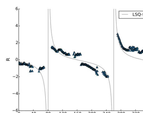
The fitting of Eq. (7) is a nonlinear optimization problem, for which the least-squares method (LSQ) was used. The task was to minimize the squared difference between data and the model values. The results of fitting Eq. (7) into the quadrant sensor data are shown in Figs. 13 and 14. The fit in Fig. 14 is not as good as in Fig. 13, because in the data of Fig. 14 there exist artifacts caused by as yet unknown reasons. In general the shape of the data in Fig. 14 seems similar to the data in Fig. 13. The values obtained for parametersA,BandC dur-ing sol intervals 1–45 and 46–376 are presented in Table 3.

After obtaining all the values for Eq. (7) parameters, the fitted tangential model is used to predict the wind directions for new values measured for the ratio of voltages R by the quadrant sensor. The calibration function defined in Eq. (7) can be used to reconstruct the wind directions during the complete VL1 mission, because only the heater element in the quadrant sensor failed. The thermocouples remained op-erating nominally; therefore, the ratioR of quadrant sensor voltages should obtain values on the same order of magnitude during the whole VL1 mission. The distributions of values, obtained forR, during sols 46–377 and 378–2245 are shown in Figs. 15 and 16, respectively. The algorithm for wind re-construction in stage 2 is similar to the algorithm presented in Algorithm 1 except that the R value is calculated using Eq. (6) instead of theF value.

4 Validation of the wind reconstruction algorithm 4.1 Error analysis of VL1 sols 1–45

The error analysis of the wind reconstruction algorithm is done by comparing the data produced by the the algorithm with the VL1 SANMET wind data. Because the VL1 wind measurement instruments remained fully functional for the first 45 sols of the VL1 mission, it is assumed that the data for that period are correct and can be used as a reference for the comparison. The behavior of the algorithm was tracked for every reconstructed sol, and data for the error analysis were gathered simultaneously with the reconstruction. The key in-dicator for the performance of the algorithm is the absolute difference between SANMET and reconstructed angles:

1θ=θSANMET−θAlgo

. (8)

0 40 80 120 160 200 240 280 320 360

Wind direction (

◦

)

6 4 2 0 2 4 6

R

LSQ-fit

Figure 13.Calibration functionRduring sols 1–45.

0 40 80 120 160 200 240 280 320 360

Wind direction (

◦

)

6 4 2 0 2 4 6

R

LSQ-fit

Figure 14.Calibration functionRduring sols 46–377.

(9)

10 5 0 5 10

R

0 5000 10000 15000 20000

Count

Figure 15.The distribution ofRvalues during sols 46–377.

10 5 0 5 10

R

0 5000 10000 15000 20000 25000 30000

Count

Figure 16.The distribution ofRvalues during sols 378–2245.

the hourly mean of the reconstructed wind speed is greater than the SANMET-determined mean value. However, the SANMET-determined mean value for wind speed is within the error limit of the reconstructed wind speed in all hours except the 20th and 21st. In Fig. 19 the hourly means of SANMET determined wind directions and speeds and the re-constructed wind directions and speeds are shown during the first 45 sols of VL1 mission. The error bars in Fig. 19 are the standard deviations of the measurements done during a specific hour. In addition to the hourly mean wind direction and speed, a point-by-point comparison between the SAN-MET and reconstructed data are shown in Figs. 20 and 21. Figure 20 presents the comparison between wind direction and speed of SANMET and reconstruction from the forenoon of sol 3. The mean absolute difference between the SAN-MET and reconstructed wind direction was 9.1◦ during the 6 min time period. The reconstructed wind speeds have a high-speed bias caused by the wind direction being almost

5

10

15

20

25

30

35

40 Sol

0

5

10

15

20

25

30 Me

an

ab

so

lut

e d

iff

er

en

ce

(

◦

)

Figure 17.The diurnal mean angle difference.

5

10

15

20

25

30

35

40 Sol

0

5

10

15

20

25

30

35 St

an

da

rd

d

ev

iat

ion

of

d

iff

er

en

ce

(

◦

)

Figure 18.The diurnal standard deviation of the angle difference.

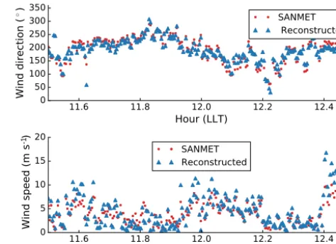
parallel to the WS1. Figure 21 displays SANMET and re-constructed wind directions and speeds during a 1 h period at the midday of sol 41. During the 1 h period, the mean ab-solute difference between SANMET and reconstructed wind directions was 12.2◦.

(10)

continu-0 4 8 12 16 20 24

Time (LLT)

0 40 80 120 160 200 240 280 320 360

Me

an

w

ind

d

ire

cti

on

(

◦

)

SANMET Reconstructed

0 4 8 12 16 20 24

Time (LLT)

0 2 4 6 8 10 12 14 M ea n w in d sp ee d (m s -1) SANMET Reconstructed

Figure 19.The hourly mean wind direction and speed from SAN-MET and reconstruction during sols 1–45 (Ls=97–118◦).

9.94 9.96 9.98 10.00 10.02 10.04

Hour (LLT)

0 50 100 150 200 250 300 350

W

ind

d

ire

cti

on

(

◦

)

9.94 9.96 9.98 10.00 10.02 10.04

Hour (LLT)

0 2 4 6 8 10 12 14

W

ind

sp

ee

d

(m

s

)

SANMET Reconstructed -1

Figure 20.Wind direction and speed during a 6 min time period from the forenoon of sol 3 (Ls=98◦).

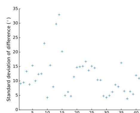
ity was applied in the reconstruction process occurred during nighttime hours (00:00–06:00), when the Sun’s radiation was not strong enough to heat the quadrant sensor. In Figs. 22 and 23, the histograms of the mean difference of reconstructed and SANMET angles as well as the standard deviation of the angle difference are presented.

4.2 Slope winds of the VL1 area

Another validation method for the reconstruction algorithm is based on the physical fact that there should exist slope winds in the reconstructed wind data. The VL1 landed on a slope rising to the south and west. In this case the slope winds in the VL1 area will form when the nocturnally cooled dense air is accelerated down the slope by gravity. Therefore, in nocturnal hours, the direction of wind should be in the in-terval 180–270◦_{, in which case the wind is from the top part}

11.6 11.8 12.0 12.2 12.4

Hour (LLT)

0 50 100 150 200 250 300 350

W

ind

d

ire

cti

on

(

◦

)

SANMET

Reconstructed

11.6 11.8 12.0 12.2 12.4

Hour (LLT)

0 5 10 15 20

W

ind

sp

ee

d

(m

s

)

Figure 21.Wind direction and speed during 1 h at the midday of sol 41 (Ls=116◦).

5 10 15 20 25 30

Mean absolute difference (

◦

)

0 2 4 6 8 10

Number of sols

Figure 22.Mean absolute difference of the angles during sols 1–45.

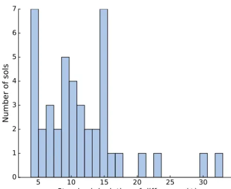
of the slope. Soon after sunrise, the direction of wind should change, so that the daytime winds are anabatic. The anabatic winds are accelerated upslope by sun-heated warm slopes. The daytime wind directions should regularly be in the inter-val 0–90◦_{. According to Figs. 19, 26 and 27, the wind} direc-tion data match the physical slope wind direcdirec-tions reason-ably well, especially during nighttime and late afternoons. The slope winds are typically observed in Martian summer as the conditions for observing the slope winds are optimal. The conditions for observing the slope wind are a terrain sloping over a large area; strong diurnal temperature variation; and weak ambient winds, which are typical on Mars in summer (Savijärvi and Siili, 1993).

(11)

recon-T. Kynkäänniemi et al.: Wind reconstruction algorithm for Viking Lander 1 227

5 10 15 20 25 30 35

Standard deviation of difference (

◦

)

0 1 2 3 4 5 6 7

Number of sols

Figure 23. Standard deviation of the angle difference during sols 1–45.

structed wind directions it is 220–230◦. Taking into account that the mean difference between SANMET wind directions and reconstructed directions was 12.8◦during sols 1–45, the locations of the peak maximums are consistent with each other. Inspecting the left-side tail of both distributions, one sees that there exists a small local maximum approximately between 80 and 100◦_{. The small local maximum is likely} caused by the daytime anabatic winds, which flow upslope.

5 Reconstructed sols of VL1

The algorithm was used to reconstruct all available VL1 sols, and the results from the reconstruction are presented in this section. The statistical distribution of wind directions is shown in a histogram in Fig. 25 to allow studying the exis-tence of slope winds in the VL1 area. In the figure the wind directions are divided into 10◦ _{sized bins. The distribution} of the wind directions determined by SANMET is shown in Fig. 25 as a comparison with the reconstructed wind tions. The SANMET method for determining the wind direc-tion is not reliable after sol 45, because it does not take into account the decay of the quadrant sensor heater element or, likewise, the failure of one of the wind sensors.

Two clear peaks are visible in Fig. 25 in the reconstructed wind directions. One peak is located between 80 and 120◦_, and the other is in interval 240–300◦_{. The peak in the angle} range 80–120◦ _{is much sharper than the peak in the range} 240–300◦. The peak in the range 240–300◦ corresponds to the nocturnal wind, which is directed downslope, and the peak in the range 80–120◦ is the daytime anabatic upslope wind.

To illustrate the reconstructed wind measurements, sols 15 and 1413 of the VL1 mission are presented in Figs. 26 and 27. These sols were selected because the first sol is from

0 40 80 120 160 200 240 280 320 360

Reconstructed wind direction (

◦

)

0 2000 4000 6000 8000 10000 12000

Count

0 40 80 120 160 200 240 280 320 360

SANMET wind direction (

◦

)

0 1000 2000 3000 4000 5000 6000 7000 8000 9000

Count

Figure 24.Statistical distributions of wind directions during VL1 sols 1–45.

0 40 80 120 160 200 240 280 320 360

Reconstructed wind direction (

◦

)

0 10000 20000 30000 40000 50000 60000 70000 80000

Count

0 40 80 120 160 200 240 280 320 360

SANMET wind direction (

◦

)

0 10000 20000 30000 40000 50000 60000 70000 80000 90000

Count

Figure 25.Comparison between SANMET and reconstructed wind direction during the complete VL1 mission.

the time when the VL1 wind measurement instruments were intact, and the second sol is from the time when the wind measurement instruments were partially decayed. The quad-rant sensor of VL1 and both of the wind sensors were in-tact during sol 15. During sol 1413, both the quadrant sen-sor heater and one of the hot-film wind sensen-sors had already failed. The season is the same in sols 15 and 1413; thus the sols should exhibit similar diurnal behavior.

(12)

0 4 8 12 16 20 24

Time (LLT)

0 40 80 120 160 200 240 280 320 360

Me

an

w

ind

d

ire

cti

on

(

◦

)

0 4 8 12 16 20 24

Time (LLT)

0 1 2 3 4 5 6 7 8 9

Me

an

w

ind

sp

ee

d

(m

s

)

Figure 26.Comparison of SANMET and reconstructed hourly wind directions and speeds for sol 15.

of the slope. After sunrise the wind rotates about 180◦_and begins to flow from the lower part of the slope.

6 Summary and discussion

The article focused on developing an algorithm to reconstruct the wind measurements during the complete VL1 mission. VL1 performed wind direction and speed measurements on the surface of Mars for 2245 sols; thus the data set produced by the wind reconstruction is significant in its size.

The wind measurement system of VL1 consisted of two orthogonal hot-film wind sensors and a quadrant sensor for solving the ambiguity in wind direction. The quadrant sensor failed during sol 45, and one of the wind sensors broke down during sol 378; thus only one of these three instruments re-mained fully intact for the VL1 mission. However, with the algorithm described in this report, it was possible to recon-struct the wind measurements with a reasonable accuracy.

The wind reconstruction was completed in two stages. In the first stage the quadrant sensor signals from sols 1–45 were used to calibrate Nusselt numbers of the hot-film wind sensors. The wind sensors were then used to estimate wind directions during sols 46–377. With the estimated wind di-rections the quadrant sensor was recalibrated and was then used to reconstruct all the wind directions from the VL1 mission. The reconstruction of wind speed was also possible with one wind velocity component and the wind direction. The results from the reconstruction of the wind speeds are not always very reliable, because the reconstruction of wind speed required knowledge of both the wind direction and the wind velocity component from the nominally working wind sensor. The wind directions contain variable amounts of error between different sols. Therefore, the reconstruction quality of the wind speed is weaker for sols with more error in the wind direction.

0 4 8 12 16 20 24

Time (LLT)

0 40 80 120 160 200 240 280 320 360

Me

an

w

ind

d

ire

cti

on

(

◦

)

Reconstructed

0 4 8 12 16 20 24

Time (LLT)

0 2 4 6 8 10 12

Me

an

w

ind

sp

ee

d

(m

s

)

Reconstructed -1

Figure 27.The reconstructed hourly wind directions and speeds for sol 1413.

The developed algorithm for wind reconstruction shows the presence of slope winds in the VL1 area. The accuracy of the algorithm compared to the data measured by fully func-tional VL1 wind measurement instruments is reasonable. On average the mean of the absolute difference between wind direction was determined to be 12.8◦.

The new wind reconstruction algorithm developed in this article extends the amount of available sols of VL1 from 350 to 2245 sols. The reconstruction of wind measurement data enables the study of both short-term phenomena, such as daily variations in wind conditions or dust devils, and long-term phenomena, such as the seasonal variations in Martian tides.

Data availability. The data are not publicly available as they are currently in an immature state but will be made completely available later on, likely through the PDS. At present the data are available upon request; please bear in mind that the data may be subject to changes.

Competing interests. The authors declare that they have no conflict of interest.

Acknowledgements. The authors are thankful for the Finnish Academy grant no. 131723.

Edited by: Valery Korepanov

(13)

T. Kynkäänniemi et al.: Wind reconstruction algorithm for Viking Lander 1 229 References

Buehler, G. D.: SD-37P0011A Viking’75 Project Program Descrip-tion Document for the Meteorology Analysis Program (SAN-MET), Project documentation, National Aeronautics and Space Administration (NASA), 1974.

Chamberlain, T. E., Cole, H. L., Dutton, R. G., Greene, G. C., and Tillman, J. E.: Atmospheric Measurements on Mars: the Viking Meteorology Experiment, B. Am. Me-teorol. Soc., 57, 1094–1104, https://doi.org/10.1175/1520-0477(1976)057<1094:AMOMTV>2.0.CO;2, 1976.

Davey, R., Chamberlain, T., and Harnett, L.: Sensor Design Analy-sis Report, TRW Systems Group, 1973.

Golombek, M. P., Anderson, R. C., Barnes, J. R., Bell III, J. R., Bridges, N. T., Britt, D. T., Brückner, J., Cook, R. A., Crisp, J. A., Economou, T., Folkner, W. M., Greely, R., Haberle, R. M., Hargraves, R. B., Harris, J. A., Haldemann, A. F. C., Herkenhoff, K. E., Hviid, S. F., Jaumann, R., Johnson, J. R., Kallemeyn, P. H., Keller, H. U., Kirk, R. L., Knudsen, J. M., Larsen, S., Lem-mon, M. T., Madsen, M. B., Magalhães, J. A., Maki, J. N., Malin, M. C., Manning, R. M., Matijevic, J., McSween, H. Y., Moore, H. J., Murchie, S. L., Murphy, J. R., Parker, T. J., Reider, R., Rivellini, T. P., Schofield, J. T., Seiff, A., Singer, R. B., Smith, P. H., Soderblom, L. A., Spencer, D. A., Stoker, C. R., Sulli-van, R., Thomas, N., Thurman, S. W., Tomasko, M. G., Vaughn, R. M., Wänke, H., and Wilson, G. R.: Overview of the Mars Pathfinder Mission: Launch Through Landing, Surface Opera-tions, Data Sheets, and Science Results, 1999.

Hess, S., Henry, R., Leovy, C. B., Ryan, J., and Tillman, J. E.: Me-teorological Results from the Surface of Mars: Viking 1 and 2, J. Geophys. Res., 82, 4559–4574, 1977.

Holstein-Rathlou, C., Gunnlaugsson, H. P., Merrison, J. P., Bean, K. M., Cantor, B. A., Davis, J. A., Davy, R., Drake, N. B., Elle-hoj, M. D., Goetz, W., Hviid, S. F., Lange, C. F., Larsen, S. E., Lemmon, M. T., Madsen, M. B., Malin, M., Moores, J. E., Nürn-berg, P., Smith, P., Tamppari, L. K., and Taylor, P. A.: Winds at the Phoenix landing site, J. Geophys. Res.-Planets, 115, e00E18, https://doi.org/10.1029/2009JE003411, 2010.

Kemppinen, O., Tillman, J., Schmidt, W., and Harri, A.-M.: New Analysis Software for Viking Lander Meteorological Data, Geo-scientific Intrumentation Methods and Data Systems, 2013. Murphy, J. R., Leovy, C. B., and Tillman, J. E.: Observations of

Martian Surface Winds at the Viking Lander 1 Site, J. Geophys. Res., 95, 14555–14576, 1990.

Newman, C. E., Gómez-Elvira, J., Marin, M., Navarro, S., Tor-res, J., Richardson, M. I., Battalio, J. M., Guzewich, S. D., Sullivan, R., de la Torre, M., Vasavada, A. R., and Bridges, N. T.: Winds measured by the Rover Environmental Moni-toring Station (REMS) during the Mars Science Laboratory (MSL) rover’s Bagnold Dunes Campaign and comparison with numerical modeling using MarsWRF, Icarus, 291, 203–231, https://doi.org/10.1016/j.icarus.2016.12.016, 2016.

Savijärvi, H. and Siili, T.: The Martian Slope Winds and the Nocturnal PBL Jet, J. Atmos. Sci., 50, 77–88, https://doi.org/10.1175/1520-0469(1993)050<0077:TMSWAT>2.0.CO;2, 1993.

Schofield, J., Barnes, J. R., Crisp, D., Haberle, R. M., Larsen, S., Magalhaes, J., Murphy, J. R., Seiff, A., and Wilson, G.: The Mars Pathfinder Atmospheric Structure Investiga-tion/Meteorology (ASI/MET) Experiment, Science, 278, 1752– 1758, 1997.

Soffen, G. A.: The Viking Project, J. Geophys. Res., 82, 3959–3970, 1977.