Lag profile inversion method for EISCAT data analysis

www.ann-geophys.net/26/571/2008/ © European Geosciences Union 2008

Annales

Geophysicae

Lag profile inversion method for EISCAT data analysis

I. I. Virtanen1, M. S. Lehtinen2, T. Nygr´en1, M. Orisp¨a¨a2, and J. Vierinen2 1_{Department of Physical Sciences, University of Oulu, P.O. Box 3000, 90014, Finland} 2_{Sodankyl¨a Geophysical Observatory, 99600, Sodankyl¨a, Finland}

Received: 16 May 2007 – Revised: 5 November 2007 – Accepted: 17 December 2007 – Published: 26 March 2008

Abstract. The present standard EISCAT incoherent scatter experiments are based on alternating codes that are decoded in power domain by simple summation and subtraction oper-ations. The signal is first digitised and then different lagged products are calculated and decoded in real time. Only the decoded lagged products are saved for further analysis so that both the original data samples and the undecoded lagged products are lost. A fit of plasma parameters can be later performed using the recorded lagged products. In this paper we describe a different analysis method, which makes use of statistical inversion in removing range ambiguities from the lag profiles. An analysis program carrying out both the lag profile inversion and the fit of the plasma parameters has been constructed. Because recording the received signal it-self instead of the lagged products allows very flexible data analysis, the program is constructed to use raw data, i.e. IQ-sampled signal recorded from an IF stage of the radar. The program is now capable of analysing standard alternating-coded EISCAT experiments as well as experiments with any other kind of radar modulation if raw data is available. The program calculates the ambiguous lag profiles and is capable of inverting them as such but, for analysis in real time, time integration is needed before inversion. We demonstrate the method using alternating code experiments in the EISCAT UHF radar and specific hardware connected to the second IF stage of the receiver. This method produces a data stream of complex samples, which are stored for later processing. The raw data is analysed with lag profile inversion and the results are compared to those given by the standard method. Keywords. Radio science (Ionospheric physics; Signal pro-cessing; Instruments and techniques)

Correspondence to: I. I. Virtanen

([email protected])

1 Introduction

In an incoherent scatter radar (ISR) experiment, a radiowave is transmitted to the ionosphere where a small fraction of the original signal is scattered to the receiver antenna. Lagged products of the received signal and its complex conjugate are calculated to produce samples of the signal autocorrela-tion funcautocorrela-tion (ACF). Then different plasma parameters (e.g. electron density and electron and ion temperatures) are de-termined from the ACF observations by means of a fitting routine.

The standard EISCAT hardware does not save the received signal itself, but calculates the lagged products in real time and saves them on hard disk after some postintegration. This process puts limits to all resolutions in further analysis, in-cluding range resolution, time resolution and lag resolution. Also, it loses the original signal so that it can no more be used in any other way and its properties cannot be investi-gated. While the lag profile inversion method discussed in this paper can be based on the lagged products, proper han-dling of some other things such as ground clutter, space de-bris/satellite echoes and other phenomena with long correla-tion times are very difficult to analyse from lag profile data. This either requires an impractically large number of lag pro-files to be stored (so that the storage requirements far exceed those for storage of the IQ-sampled signal itself) or the phe-nomena are actually only sub-optimally resolved from the correlated (lag profile) data.

et al., 2000; Grydeland et al., 2005c). Saving the digitised signal may even allow the data to be used for new purposes, such as accurate meteor-head measurements (Sulzer, 2004), but still standard ion line measurements often save only the lagged products.

The standard tool for analysing the EISCAT data is the GUISDAP package (Lehtinen and Huuskonen, 1996). The analysis is based on the concept of range-gates in the follow-ing way: The user can choose a series of range-gates which are consecutive range intervals defining the range resolution of the analysis. It is then assumed that the plasma prop-erties inside each range-gate correspond to a single set of plasma parameters. The range- and lag-coverages of individ-ual lagged products are expressed in terms of the correspond-ing ambiguity functions. The concept of ambiguity functions is introduced e.g. by Lehtinen and Huuskonen (1996). All lagged products whose range ambiguity function mainly fit inside a range-gate (is zero-valued outside the gate) are then chosen as the data for the parameter fit of the gate. Because of the assumption of a single set of plasma parameters be-longing to the range-gate, the forward model in the parameter fit (ACF as a function of known plasma parameters) can be simply based on lag ambiguity functions. Thus, a set of esti-mated plasma parameters is produced for each range-gate.

Full profile analysis, which is described in Lehtinen et al. (1996), differs from standard analysis in the sense that no as-sumptions of piecewise constant plasma parameters are done. Instead, it is assumed that the plasma parameters are mod-elled as a spline expansion with user-defined nodes specify-ing the (possibly differspecify-ing) range resolutions of the plasma parameters. All measured correlation estimates (lagged products) are then fitted to theoretically calculated values using two-dimensional (range and lag) ambiguity functions. This kind of model is much less approximative than the range-gate assumption in standard analysis. Full profile anal-ysis also allows different kinds of resolution assumptions for different parameters. The analysis is computationally much more expensive than standard GUISDAP analysis and some hand-tuned shortcuts had to be used (Lehtinen et al., 1996) to make it possible to get results with the computers avail-able at that time. This is the main reason why it could not be developed into a general-purpose analysis tool.

The analysis described in this paper is performed actually in two steps: The first step is a linear inversion of ambiguous lagged products to a sequence of lag profiles with a user-chosen lag and range resolution. The second step is a non-linear inversion of the plasma parameters. This approach has the following advantages:

1. The first step in the inversion is linear, which makes the analysis much faster than the full profile analysis. 2. The two-stepped approach separates the technically

complicated questions related to radar coding from those related to plasma physics models. Different kinds of plasma spectrum models can easily be applied in the

second step with no need to repeat the first step. Thus the scientist doing the analysis does not need to fully un-derstand all the details of radar coding theory, and can concentrate on the physical aspects of plasma spectra. The purpose of the present paper is to demonstrate the lag profile inversion and the whole sequence of IS data analysis from raw data up to the final parameter fit. All data analysis routines described in this paper are collected in an analysis package written in Fortran 95. Most of the methods have been presented in earlier publications (Lehtinen et al., 2002; Damtie et al., 2002, 2004) but never collected together into this kind of package. The package is still under develop-ment, but it is already capable of performing the whole pro-cedure including the parameter fit. Inversion methods have also been used to improve zero lag accuracy of multipulse experiments (Lehtinen and Huuskonen, 1986). Another in-version based analysis method is also being developed using data from Arecibo (Nikoukar et al., 20081_{), where linear} in-version methods are also used for measuring vector velocities (Hagfors and Behnke, 1974; Sulzer et al., 2005).

We apply lag profile inversion to data obtained from stan-dard alternating code experiments. In principle, lag profile inversion works with any phase coded transmissions. This allows one to search for new kinds of radar codes without any special decoding method applied to them, which is the main reason to build the new analysis package. A decoding filter based method for deconvolving lag profiles from practically any phase code has been discussed already by Sulzer (1989). In fact code sequences with similar estimation accuracy with alternating codes but with smaller number of different codes have been found, these new codes remain to be published in a separate paper.

2 Lag profile analysis

In standard analysis of alternating codes, a set of lag pro-files with different lag values (i.e. range propro-files of certain lagged products) are first calculated for each transmission of the code cycle, and decoding is then made by means of addi-tions and subtracaddi-tions which are specific to the applied code. Before decoding, the calculated lag values are convolutions of the true lag profile and a range ambiguity function. The task of decoding is to produce lag profiles with a range reso-lution determined by the length of the bit in the code.

can be found from several books, e.g. Tarantola (1998, 2005); Menke (1989); Kaipio and Somersalo (2005).

When raw data is analysed, the theoretical limits of lag and range resolutions depend on the sampling frequency. Any lag valueτ that is a multiple of the sampling interval can be calculated, i.e. the possible lags are

τ = N fs

, (1)

whereN=0,1,2, . . .andfs is the sampling frequency.

Cor-respondingly, the possible widths of range-gates are 1r=K c

2fs

, (2)

whereK=1,2,3, . . .andcis the speed of light.

Both range and time integration can be performed to im-prove the accuracy of the ACF estimates. In the lower E region the basic range resolution of the experiment (the bit length when using alternating codes) may be useful, but above E region some range integration can be performed to stabilise the solution and to reduce the computing time. The software puts no limits to the integration time, if the fact that at least a single transmission is needed is not counted as a limitation. The true lower limit of the integration time arises from the statistical nature of the measurement: the number of measured samples must be large enough to produce a good estimate of the true lag value.

2.1 Recording

Data from two different experiments are analysed in this pa-per. Both of them are based on 64-bit alternating codes, and they were run on 2 October 2005 and on 25 November 2006. The data were collected using extra receiving devices syn-chronised with the radar clock and connected to the second IF stage of the EISCAT UHF receiver. The exact frequency of the IF signal depends on the applied frequency channel, but its value is about 10 MHz. The receiving hardware was different in the two cases but, effectively, it carried out down-conversion to the baseband as well as complex sampling. Both real and imaginary parts were written to hard disk for later analysis. The data contains not only the scattering sig-nal but also the true attenuated transmitted wave form.

A description of the recording system used on 2 Octo-ber 2005 is given by Markkanen et al. (2005). The bit length of the alternating code was 6 µs. The effective sam-pling frequency on the base band was 500 kHz, which corre-sponds to a sampling interval of 2 µs and a range resolution of 300 m. The basic height resolution of conventional decoding is 900 m. The oversampling of the signal allows the calcula-tion of fraccalcula-tional lags, which can reduce the variance of the results by a factor close to 1.5 (Huuskonen et al., 1996).

On 25 November 2006 the data were sampled using Na-tional Instruments PXI-5142 OSP high speed digitizer. The bit length of the alternating code was 3 µs, which leads to a

450-m range resolution in conventional analysis. The effec-tive sampling frequency on the base band was 1 MHz. 2.2 Clutter suppression

Incoherent scatter experiments may be contaminated by ground clutter, i.e. coherent echoes from ground or sea. This is not serious, if the radar site is surrounded by close-by mountains like at Tromsø, where the EISCAT UHF and VHF radars are located. On Svalbard, however, the ESR radar suf-fers from clutter originating at long ranges and disturbing the lowest parts of the lag profiles.

The clutter signal can be filtered out because it has a very long correlation time compared to that of the ionospheric scattering signal. One way to remove clutter is to subtract two sample profiles before calculating the lagged products in real time. Then, in effect, one half of the measurements are lost, which reduces the accuracy of the results. For the stan-dard method of clutter removal in the ESR radar, see Turunen et al. (2000).

Storing the raw data instead of ACF estimates gives a pos-sibility of a better clutter removal (Lehtinen et al., 2002). An average of recorded echoes over several similar transmis-sions is first calculated. Due to the long correlation time of clutter, the clutter signal remains unaffected in the average, but the mean value of the scattering signal approaches zero. When the average signal profile is subtracted from one of the signals used in the average, the coherent clutter echoes are removed, and a clean signal is obtained for later processing. Depending on the number of signals that can be included in the average, the clutter suppression affects to the signal statistics by varying amount. Because lag profile inversion calculates variances for the inverted lag profiles, the possible deterioration in signal statistics will be readily seen as larger variance in the inverted lag profile.

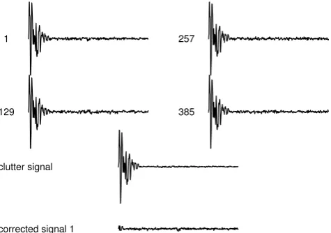
The clutter removal is demonstrated in Fig. 1. Here 512 signal profiles from the experiment run on 2 October 2005 are used. Since the 64-bit alternating code sequence contains 128 different transmission envelopes, every 128th transmis-sion is taken into the average. Figure 1 shows lower parts of four signal profiles, the clutter profile obtained as an av-erage of 4 profiles, and the first signal profile after clutter correction. This small number is dictated by the length of the alternating code sequence and the correlation length of the clutter signal. As a matter of fact, the number of sig-nal profiles taken into the average should be great enough to make the mean value of the incoherent scatter signal ap-proach zero. As seen in Fig. 1, this does not happen with four profiles. However, with the new coding method that al-lows shorter code sequences to be used, this can be easily achieved.

1 257

129 385

clutter signal

corrected signal 1

Fig. 1. Method for clutter suppression: numbered signals are clutter

contaminated echoes of the same phase code. Due to the use of 64-bit alternating codes the same code is repeated after 128 transmis-sions. The clutter signal is produced by calculating a point-by-point average of the numbered signals. Because of the long correlation time of the clutter signal it is not averaged to zero as the true iono-spheric echoes do. The corrected signal is a clutter corrected version of signal number 1. It is produced by subtracting the clutter signal from the clutter-contaminated one. To make the clutter correction for signal 2 an average of signals 2, 130, 258 and 386 is subtracted from signal 2 etc.

fact, the analysis package contains options with or without clutter removal.

2.3 Channel separation

Since our reception systems take samples of the signal from the second IF stage, the recorded data stream contains all frequency channels that were used in the experiment. The channels must be separated in the analysis, and data from each channel must be included in lag profile inversion. The channel separation is performed by complex mixing and fil-tering. A signal at frequencyωj is mixed to zero frequency

by multiplying it with exp(−iωjt ), wheretis time. Signals

at other frequencies are filtered out using a simple low-pass boxcar filter. At this point it is also possible to reduce the number of data samples by means of decimation to make the analysis faster.

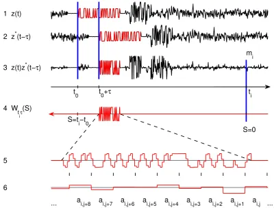
2.4 Ambiguous lag profiles and ambiguity functions After channel separation the data is ready for actual lag pro-file analysis. In channel separation the transmission fre-quency is mixed to zero, which means that the transmission part of the data has the shape of the modulation envelope. This is demonstrated with real data from the 2 October 2005 experiment on line 1 in Fig. 2, where the transmission part of the signal is marked with red colour.

The first task in lag profile analysis is to calculate the lagged products z(t )z∗(t−τ ) of the complex signal z(t ), whereτ is the lag increment, and the range ambiguity func-tion

Wt τ(S)=(p∗env)(t−S)(p∗env)∗(t−τ −S). (3)

HereSis the time from the start of transmission to the instant of reception,pis the receiver impulse response and env is the transmission envelope (Lehtinen and Huuskonen, 1996). In the standard analysis, theoretical modulation envelopes are used in calculating the ambiguity functions. Since our data contains the true envelopes, we can also use the true ambigu-ity functions.

If the lagged product z(t )z∗(t−τ ) is calculated for the whole data vector containing the measured transmission en-velope, both the lagged product of the scattering signal and the range ambiguity function are created at the same time. The non-zero part of the product(p∗env)(t )(p∗env)∗_{(t−τ )}

will be produced at the part of the lag profile where the data vector contains the transmission envelope. In the echo part of data this product is known to be zero, because the transmit-ter is off and thus env(t )=0. This is demonstrated in Fig. 2. There line 1 contains an individual sampled signal profilez as a function of timet and line 2 the same profile shifted in time by an amountτ (only real parts are shown for conve-nience). The transmission starts att=t0. Line 3 is the real part of the productz(t )z∗(t−τ )(this is affected also by the imaginary parts which are not shown). On line 3, the range ambiguity function for lagτ, i.e.Wt τ(S), appears in the

bot-tom part of the profile and is marked by red line (at other instances of timeWt τ(S)=0).

The non-zero part of the range ambiguity functionWtiτ(S) has a similar shape for all reception timesti. Obviously there

is a shift towards larger ranges (larger values ofS) as the time increases and the transmitted pulse proceeds further away from the radar. At timeti the range coordinate of a signal

transmitted at timet0isti−t0(see line 4 in Fig. 2). In other words, the positive direction of the range axis is to the left in the figure (opposite to the time axis) and the zero range is located atti. In this way the range ambiguity function for

any lagged product can be easily constructed. 2.5 Power calibration

For calibration purposes, a noise injection is added after ev-ery second transmission. The injection power is obtained by subtracting the average power (i.e. the zero lagz(t )z∗(t )) of the pure background signal from the power of the signal with noise injection. All lag profiles were divided by the injection power in order to have them in the same power scale.

1 z(t)

2 z*(t−τ)

m_i

3 z(t)z*(t−τ)

t₀ t₀+τ t_i

4 W_t

iτ

(S)

S=t_i−t₀

S=0

5

a_i,j+8 a_i,j+7 a_i,j+6 a_i,j+5 a_i,j+4 a_i,j+3 a_i,j+2 a_i,j+1 a_i,j 6

... ...

Fig. 2. Producing the linear coefficients for lag profile inversion: On line 1 is a short time sequence of the received signal containing one

transmission (marked with red color). On line 2 is the complex conjugate of the signal shifted by the lag-incrementτ. By multiplying 1 and 2 both the lag profile and range ambiguity function (the red part of the curve) are produced. The range ambiguity function is in a coordinate system with positive S-axis to left in the figure and the origin (S=0) at the pointt=ti (ti is the instant of time when the ambiguous lagged

productmiwas measured). On line 5 is a blow-up of the non-zero part of the range ambiguity function. The limits of range-gates are marked

with black vertical bars between lines 5 and 6. All points of the range ambiguity function that lie inside the same gate are summed together to produce the linear coefficientsai,kon line 6.

2.6 Lag profile inversion

The next step in the analysis is to produce unambiguous lag profiles from the measured lagged products by means of lag profile inversion. Due to the length of the transmitted pulses, the original lagged products have contribution from long range intervals. In the conventional analysis of alternat-ing codes, a range resolution correspondalternat-ing to the length of a single bit in the code is obtained by means of decoding which is made in power domain. Lag profile inversion can do the same without using the specific properties of the alternating codes. A key point in lag profile inversion is that unknowns, measurements and measurement errors are all treated as ran-dom variables.

Range integration is often used in order to improve statis-tical accuracy at altitudes where the plasma parameters can safely be modeled to be constant over larger range intervals than the basic range resolution of the experiment. In standard analysis, this is simply done by adding decoded lag values of

subsequent ranges in the profile and, as a result, the range-gates will be longer than in the basic analysis. In the case of the lag profile inversion method, the range-gates can be cho-sen before the inversion as demonstrated by lines 5 and 6 in Fig. 2. Range integration both makes the lag profile inversion more stable and reduces the computing time.

The tick marks on line 5 of Fig. 2 indicate the boundaries of chosen range-gates. Because it is assumed that the ACF at lagτ is constant within each range-gate, a measured am-biguous lagged productmi has a certain contribution from

true lag valuesxkin each gatek. This contribution is the

un-known true lag valuexk multiplied by the integral of range

ambiguity functionWti,τ(S)over the range-gatek. Thus the measured ambiguous lagged product is sum of all these con-tributions:

mi = N

X

j=1

whereNis the total number of range-gates andεithe error in

theith measurement. Because the transmitted pulse usually covers only small part of the range-gates at a time, many of the coefficientsai,j in Eq. (4) are zeros. The coefficients

have to be re-calculated for each lagged product, because the range ambiguity function moves with respect to the limits of the chosen range-gates. When all measurements and errors are collected into column vectors, they can be presented in terms of a matrix equation

m=Amx+ε, (5)

where

m=(m1, m2, . . . , mM)T (6)

is the measurement vector,

Am=



 

a1,1 . . . a1,N

..

. . .. ... aM,1. . . aM,N





 (7)

is the theory matrix,

ε=(ε1, ε2, . . . , εM)T (8)

is the error vector andMis the number of measured ambigu-ous lagged products for lagτ. HereT means transpose so thatmandεare column vectors. Many experiments contain transmissions in several frequency channels. In lag profile inversion the channels do not need to be decoded one-by-one as in standard decoding of alternating codes, but all measure-ments can be collected into the same matrix equation. In this way only one ACF per integration period is produced. This property of the method is not demonstrated in the present paper, because both experiments contain only a single fre-quency channel.

Though additional information is not needed to solve the inversion problem, the program contains an optional regular-isation routine, i.e. a method for using information not origi-nating from the measurement itself to stabilise the inversion result. The routine is implemented by expanding Eq. (5) in the following manner.

If we assume that the true lag values in range-gatesj and j−1 are the same, we make an errorεr,j. This can be written

as

0=xj−xj+1+εr,j. (9)

In addition, we can assume that the signal at the lowest gate is non-correlating noise so that the measured lag estimate only consists of a random errorεr0. This leads to a condition for boundary regularisation, i.e.

0=x1+εr0. (10)

Since Eqs. (9) and (10) are mathematically similar to Eq. (4), they can be considered as a fictitious measurements with a regularisation measurement vector

0=(0,0,· · ·,0)T (11)

and a regularisation error vector

εr =(εr1, εr2. . . , εr(N−1), εr0) (12) Thus Eqs. (4), (9) and (10) can be collected into a single matrix equation

mf =Afx+εf, (13)

where

m_f =

m

0

, (14)

εf =

ε εr (15) and

Af =

               

a1,1 a1,2 . . . a1,N−1 a1,N

..

. ... . .. ... ... aM,1aM,2. . . aM,N−1aM,N

1 −1 . . . 0 0

0 1 . . . 0 0

..

. ... . .. ... ...

0 0 . . . −1 0

0 0 . . . 1 −1

1 0 . . . 0 0

                . (16)

This regularisation method should be understood as an exam-ple of how any additional information can be easily included in the inversion. We are aware that this particular method can cause bias to the inverted lag profiles. Due to the risk of biasing and the fact that inversion works without regularisa-tion, the routine is not normally used. Anyhow, in the same way a different regularisation method or any other additional information could be included in the inversion.

The idea of lag profile inversion is to solve the most proba-ble values and posteriori variances of the unknownsxj, when

the measurementsmi and their variances are known. This is

formally a straightforward operation, provided the measure-ment errors are Gaussian. With this assumption, the posteri-ori distribution of the unknowns is also Gaussian and it can be determined. Finding a maximum of the posteriori distri-bution leads to the most probable unknown vector

x0=Q−1ATf6

−1_m

f, (17)

where

6= hεfεTfi (18)

is the error covariance matrix and

Q=AT_f6−1Af (19)

is the Fisher information matrix. The posteriori variances of the unknowns are given by

Sinceεandεrdo not correlate, the covariance matrix can be

presented in the form

6=

6m 0

0 6r

, (21)

where6mand6r are the covariance matrices ofεandεr,

respectively.

Equation (17) would give solution of the inverse problem (13), but the matrices are far too large to be handled in a straightforward manner. In practical data analysis the prob-lem is solved with a special software package for large lin-ear inverse problems, FLIPS (Fortran Linlin-ear Inverse Problem Solver). The whole theory matrix is not produced at once, but FLIPS allows one to produce only one row of the matrix, then add it to the inversion with the corresponding measurement, and finally remove the added row from computer memory. In this way very large linear inversion problems can be solved without running into problems with the computer memory size.

FLIPS uses Givens rotations to calculate the QR-decom-position (see e.g. Golub and Van Loan, 1989) of the matrix Af and hence reduces Eq. (13) to a simple form

y=Rx, (22)

where R is a square N×N upper triangular matrix. This equation is easy to solve using back substitution. FLIPS constructs implicitly the orthogonal part of the QR-decomposition and the upper triangular part row-by-row. This makes it possible to feed matrix Af into FLIPS in small

blocks (in this case one row at a time), which reduces the computer memory footprint. The measurement errors are also embedded in Eq. (22) in such a way that the posteriori covariance of the unknowns is given simply by

6=R−1(R−1)T. (23)

A single received signal profile is not sufficient for obtaining reliable ACF estimates, but some time integration is needed. For example the number of lagged products produced by a normal E-region experiment with integration time of 4 s could be of the order of 105 for a single lag and the corre-sponding theory matrix would have an equal number of rows. Because the solving method used by FLIPS allows the the-ory matrix to be produced row-by-row, so that only single row of the matrix exists in the computer memory at a time, there is no limitation for the problem size. At the moment the program is capable of performing the analysis as described above, but it is too time consuming for real-time analysis. The solution is to calculate averages of the range ambiguity functions and lag profiles before lag profile inversion. Stan-dard deviations are also calculated for the averages to be used in the inversion. Furthermore, the error distibutions will also be approximately Gaussian, as indicated by the central limit theorem, and therefore the basic assumptions in the lag pro-file inversion method will be valid. Because results of

dif-ferent phase codes cannot be averaged, the number of aver-aged measurements is proportional to the number of different codes in the experiment.

3 Parameter fit

Ionospheric plasma parameters can be solved from the decoded autocorrelation functions by fitting a theoretical plasma spectrum to a measured ACF. The spectrum and the ACF are a Fourier transform pair that makes it easy to con-vert spectra to ACFs and vice versa.

The actual fitting is performed by means of an iterative Levenberg-Marquardt algorithm that is used to find the most probable values of the ionospheric parameters and their stan-dard deviations. The direct theory (the spectrum correspond-ing a certain set of parameters) is calculated uscorrespond-ing a For-tran 95 module based on the GUISDAP routines written in C and Matlab.

4 Comparison with GUISDAP results

In order to demonstrate the applicability of the lag profile inversion method, raw data was recorded from several hours of standard EISCAT experiments with alternating codes on 2 October 2005 and 25 November 2006 in parallel with the standard recording. This gives a possibility to compare both the autocorrelation functions and the fitted parameters of the two analysis methods.

4.1 Autocorrelation functions

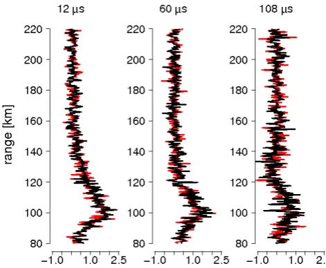
Comparisons between the lag profile inversion method and the standard alternating code decoding were made by calcu-lating different lag profiles with equal range and time res-olutions. To make a fair comparison, fractional lags were not used in the lag profile inversion. The data was also fil-tered with a 3 µs boxcar filter and decimated so that the final sampling interval is 3 µs. In this way the data used in lag pro-file inversion should be very much similar to that used in the standard analysis, the main difference being that the standard filter has a more complicated impulse response than the box-car shape. Figure 3 shows real parts of sample profiles at lags 12, 60, and 108 µs from the experiment run on 25 November 2006. The basic range resolution of the alternating code (i.e. 450 m) is used, and the time resolution is 6 s. The decod-ing results are shown by a red line and the results given by lag profile inversion by a black line. The two methods obvi-ously give similar profiles with variances of the same order of magnitude. One should notice here that the profiles are not expected to be identical, since the two methods are quite different.

Fig. 3. Real parts of sample lag profiles at 12, 60 and 108 µs from

25 November 2006. The decoding results are shown by red line and the inversion results by black line. The integration time is 6 s, the range resolution is 450 m and the ACF value is given in arbitrary units.

two methods are nearly identical and the variances, which are seen as fuzzy structures in the colour plots, are also quite similar.

4.2 Fitted parameters

For comparison of the fitted parameters given by the two methods, full autocorrelation functions were calculated by means of lag profile inversion. The range-gates were taken to be the same as in standard GUISDAP analysis. A theoret-ical plasma spectrum was fitted to the ACFs in order to find the plasma parameters. The results can then be compared with those obtained from standard GUISDAP analysis. Due to the lack of power calibration, the ACFs of the lag profile inversion method were scaled to make the resulting electron density scale match the GUISDAP density scale. The other parameters are only very weakly connected to electron den-sity, and they are expected to be correct even if the scaling of electron density would be slightly inaccurate.

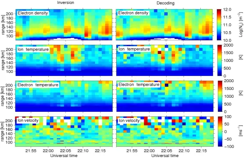
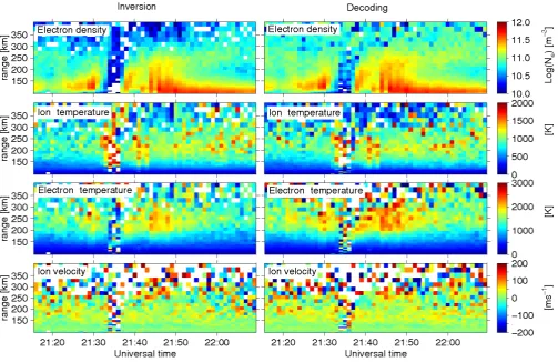
Figure 5 shows results from the observation period in Fig. 4. The standard GUISDAP results are shown on the left and the lag profile inversion results on the right hand side. The plasma parameters, from top to bottom, are elec-tron density, ion temperature, elecelec-tron temperature and ion velocity. The time resolution is 1 min and the range resolu-tion is variable so that a high resoluresolu-tion is used at low alti-tudes but higher up, were the measurements are more noisy, the resolution is lower. In general, the results given by the two methods are quite similar, although differences at cer-tain points do occur. One should notice that both methods produce occasionally pixels which do not fit in the surround-ing profile, but they are usually at different places.

A second example of comparison is shown in Fig. 6 in the same format as in Fig. 5. This is a 53-min period from 2 October 2005. Again here the same characteristics are vis-ible in both results, although minor differences are seen. A decrease in electron density is visible around 21:35 UT. At this time the profiles of other parameters become very noisy and unreliable because the scattering signal is weak due to the low electron density.

5 Discussion

The comparisons of the two data-analysis methods shows that the lag profile inversion method is capable of producing results that agree well with the results of the present standard methods. There are differences, especially when the results are noisy, but this is to be expected, because the two analysis methods are completely different.

A major advantage of recording the raw data is the possi-bility to choose the time and range resolutions of the analysis after running the experiment. In this paper the same resolu-tions as in standard analysis were chosen only to allow the comparison between the two methods. When the transmis-sion wave form is recorded along the data, the way of calcu-lating the range ambiguity functions is extremely straightfor-ward. The method virtually eliminates any possibility of er-rors due to wrongly interepreted experiment timing and other experiment details. We feel this is maybe the strongest argu-ment for storage of the data as nonprocessed echoes instead of a rather complicated set of integrated lag profiles. In the GUISDAP package a major part of the software complexity was necessitated by the need to keep record of the set of lag profiles calculated. Special initialisation calculations were necessary to model the correlator memory structure for each experiment before it could be analysed, while the present method is completely free of such complications. The way of calculating the range ambiguity functions from recorded data also makes the method quite insensitive to possible phase er-rors and power variations in the transmitted pulses.

The range-gates should be chosen so that the assumption of constant plasma parameters within each gate is a good ap-proximation. Instead of assuming the parameters to stay con-stant inside each gate, one could also use lag values in dis-crete points as unknowns and assume a linear trend between adjacent points. In future the program may be changed to use the latter choice.

The present results of the lag profile inversion were not ab-solutely calibrated but they were just roughly scaled to match with the electron densities of the GUISDAP results of the same experiment. A calibration method utilising ionosonde or plasma line data, such as that in the present GUISDAP analysis, could be implemented in the program.

Fig. 4. Real part of 12 µs lag from the same experiment as in Fig. 3 (25 November 2006). The ACF value is in arbitrary units, the time

resloution is 6 s and the range resolution 450 m.

Fig. 5. Fitted plasma parameters by means of the inversion method and standard decoding with GUISDAP. The time period is the same as in

Fig. 4 (25 November 2006).

the same estimation accuracy as alternating codes, but con-sist of only few modulation envelopes have actually been found. The theory behind these new codes and introduction

Fig. 6. Fitted plasma parameters by means of the inversion method and standard decoding with GUISDAP. The time period is from 2 October

2005.

6 Conclusions

We have shown that the lag profile analysis based on statis-tical inversion is capable of producing autocorrelation func-tions that match well with the results of decoding the alter-nating code data. Ionospheric plasma parameters have also been succesfully fit to the measured ACFs.

The new method allows one to choose the integration time and range-gates of the experiment afterwards when raw data are available. Recording the IQ-samples also gives a possibility to make detailed checks of the data quality be-fore the analysis. For instance, the shape of the transmitted pulses and amplitude of clutter signal can easily be seen. On the other hand, the use of recorded transmission envelopes makes the method less sensitive to possible errors in trans-mitted pulse shapes.

Our general view is that the lag profile inversion method allows a more flexible analysis in comparison with the tra-ditional methods. Especially, the lag profile inversion offers a possibility to use new types of phase codes with a simi-lar efficiency as the alternating codes but with a short code sequence.

Acknowledgements. The FLIPS package is free software under the terms of GNU General Public License as published by the Free Soft-ware Foundation. The program source code can be downloaded from http://mep.fi/mediawiki. The EISCAT measurements were made with special program time granted for Finland. EISCAT is an international association supported by China (CRIRP), Finland (SA), Japan (STEL and NIPR), Germany (DFG), Norway (NFR), Sweden (VR) and United Kingdom (PPARC). This work was sup-ported by the Academy of Finland (application number 213476, Finnish program for Centres of Excellence in Research 2006–2011 and application number 43988, EISCAT Data Analysis and Re-search) and by the Space Institute at the University of Oulu. The development of FLIPS package is supported by Tekes (Finnish Funding Agency for Technology and Innovation, Technology Pro-gramme MASI – Modeling and simulation 2005–2009, Research Project MASIT03 – Inversion Problems and Reliability of Models). I. Virtanen’s work was supported by the Finnish Graduate School in Astronomy and Space Physics. The authors are grateful to R. Kuula for the GUISDAP analysis of the data.

References

Chau, J. L. and Woodman, R. F.: Observations of meteor-head echoes using the Jicamarca 50MHz radar in interferometer mode, Atmos. Chem. Phys., 4, 511–521, 2004,

http://www.atmos-chem-phys.net/4/511/2004/.

Damtie, B., Nygr´en, T., Lehtinen, M. S., and Huuskonen, A.: High resolution observations of sporadic-E layers within the polar cap ionosphere using a new incoherent scatter radar experiment, Ann. Geophys., 20, 1429–1438, 2002,

http://www.ann-geophys.net/20/1429/2002/.

Damtie, B., Lehtinen, M., and Nygr´en, T.: Decoding of Barker-coded incoherent scatter measurements by means of mathemati-cal inversion, Ann. Geophys., 22, 3–13, 2004,

http://www.ann-geophys.net/22/3/2004/.

Djuth, F. T., Sulzer, M. P., and Elder, J. H.: High resolution observa-tions of HF-induced plasma waves in the ionosphere, Geophys. Res. Lett., 17, 1893–1896, 1990.

Djuth, F. T., Sulzer, M. P., and Elder, J. H.: Application of the coded long-pulse technique to plasma line studies of the ionosphere, Geophys. Res. Lett., 21, 2725–2728, 1994.

Golub, G. H. and Van Loan, C. F.: Matrix Computations, The Johns Hopkins University Press, Baltimore and London, 2nd edn., 1989.

Grydeland, T., Blixt, E., Løvhaug, U., Hagfors, T., La Hoz, C., and Trondsen, T.: Interferometric radar observations of filamented structures due to plasma instabilities and their relation to dy-namic auroral rays, Ann. Geophys., 22, 1115–1132, 2004, http://www.ann-geophys.net/22/1115/2004/.

Grydeland, T., Chau, J. L., La Hoz, C., and Brekke, A.: An imaging interferometry capability for the EISCAT Svalbard Radar, Ann. Geophys., 23, 221–230, 2005a.

Grydeland, T., La Hoz, C., Belyey, V., and Westman, A.: A proce-dure to correct the effects of a relative delay between the quadra-ture components of radar signals at base band, Ann. Geophys., 23, 39–46, 2005b.

Grydeland, T., Lind, F. D., Erickson, P. J., and Holt, J. M.: Software Radar signal processing, Ann. Geophys., 23, 109–121, 2005c. Hagfors, T. and Behnke, R. A.: Measurement of three-dimensional

plasma velocities at the Arecibo Observatory, Radio Sci., 9, 89– 93, 1974.

Holt, J. M., Erickson, P. J., Gorczyca, A. M., and Grydeland, T.: MIDAS-W: a workstation-based incoherent scatter radar data ac-quisition system, Ann. Geophys., 18, 1231–1241, 2000, http://www.ann-geophys.net/18/1231/2000/.

Huuskonen, A., Lehtinen, M. S., and Pirttil¨a, J.: Fractional lags in alternating codes: Improving incoherent scatter measurements by using lag estimates at noninteger multiples of baud length, Radio Sci., 31, 245–262, doi:10.1029/95RS03157, 1996. Kaipio, J. and Somersalo, E.: Statistical and Computational Inverse

Problems, Springer, 2005.

Lehtinen, M., Markkanen, J., V¨a¨an¨anen, A., Huuskonen, A., Damtie, B., Nygr´en, T., and Rahkola, J.: A new incoherent scat-ter technique in the EISCAT Svalbard Radar, Radio Sci., 37, 3–1, doi:10.1029/2001RS002518, 2002.

Lehtinen, M. S. and Huuskonen, A.: General incoherent scatter analysis and GUISDAP, J. Atmos. Terr. Phys., 58, 435–452, 1996.

Lehtinen, M. S. and Huuskonen, A.: The use of multipulse zero lag data to improve incoherent scatter radar power profile accuracy, J. Atmos. Terr. Phys., 48, 787–793, 1986.

Lehtinen, M. S., Huuskonen, A., and Pirttil¨a, J.: First experiences of full-profile analysis with GUISDAP, Ann. Geophys., 14, 1487– 1495, 1996,

http://www.ann-geophys.net/14/1487/1996/.

Markkanen, J., Lehtinen, M., and Landgraf, M.: Real-time space debris monitoring with EISCAT, Adv. Space Res., 35, 1197– 1209, doi:10.1016/j.asr.2005.03.038, 2005.

Menke, W.: Geophysical Data Analysis: Discrete Inversion Theory, Academic Press. Inc., San Diego, California, 1989.

Sulzer, M. P.: Recent incoherent scatter techniques, Adv. Space Res., 9, 153–162, doi:10.1016/0273-1177(89)90353-0, 1989. Sulzer, M. P.: Meteoroid velocity distribution derived from head

echo data collected at Arecibo during regular world day observa-tions, Atmos. Chem. Phys., 4, 947–954, 2004,

http://www.atmos-chem-phys.net/4/947/2004/.

Sulzer, M. P., Aponte, N., and Gonz´alez, S. A.: Application of linear regularization methods to Arecibo vector velocities, J. Geophys. Res. (Space Physics), 110, 10 305, doi:10.1029/ 2005JA011042, 2005.

Tarantola, A.: Inverse Problem Theory, Methods for Data Fitting and Model Parameter Estimation, Elsevier Science B.V., 1998. Tarantola, A.: Inverse Problem Theory and Methods for Model

Pa-rameter Estimation, Society of Industrial and Applied Mathemat-ics, 2005.

Turunen, T., Markkanen, J., and van Eyken, A. P.: Ground clutter cancellation in incoherent radars: solutions for EISCAT Svalbard radar, Ann. Geophys., 18, 1242–1247, 2000,