Listing and delisting thresholds under the Endangered Species Act
Charles Sims, David Finnoff, Alan Hastings, and Jacob Hochard*
Abstract. We consider the case where a species provides a flow of economic benefits, is at risk of extinction, and is being considered for addition to the Endangered Species List. Listing the species as endangered is costly but increases the flow of social benefits and reduces the likelihood of extinction. If the species recovers sufficiently additional costs can be incurred to subsequently delist the species. By treating listing and delisting as a pair of linked investment options, we provide an alternative to current practice for listing and delisting decisions that maximizes the return from public conservation investments. Under this alternative framework, we show that economic considerations may actually afford greater protection for at-risk species if these decisions are initiated early.
However, biological sources of uncertainty may cause species most in need of protection to be passed over in favor of more stable species that represent a “sure bet” for species preservation.
Keywords: endangered species, compound option, optimal switching, uncertainty, irreversibility
JEL Codes: D81, Q57, Q58
*
Sims ([email protected]) is a Faculty Fellow at the Howard H. Baker Jr. Center for Public Policy and an assistant professor in the Department of Economics at the University of Tennessee, 1640 Cumberland Ave, Knoxville, TN 37996. Finnoff ([email protected]) is an associate professor in the Department of
Economics and Finance, University of Wyoming. Hastings ([email protected]) is a professor in the Department of Environmental Science and Policy, University of California – Davis. Hochard
2
The listing and delisting of species as endangered, following the Endangered Species Act (ESA) of 1973, are among the highest profile, most contentious decisions made in
ecological conservation (Brown and Shogren 1998). Species survival and persistence is placed over all other concerns with a listing decision and these considerable protections are removed with delisting. The precautionary principle best describes the actual statutory language of the ESA (Prato 2005) by emphasizing the regret caused by
unexpected extinction (Bishop 1978;Ready and Bishop 1991). In practice, many species qualify for listing but remain unprotected due to limited budgets (Federal Register 2010;van Kooten and Bulte 2000). Listing and delisting criteria based on the precautionary principle are also difficult to quantify which leads to persistent debate surrounding these decisions (Doremus 1997;Robbins 2009;Shogren, et al. 2001). Cost-effectiveness criteria (Weitzman 1998;Weitzman 1993) attempt to maximize returns from public investments in conservation. This provides an alternative criterion for listing and delisting decisions that is easy to quantify and accounts for limited budgets but is
criticized for oversimplifying ecological considerations (van der Heide, et al. 2005). Furthermore, sunk transaction costs introduce the possibility of additional regret which works to discourage public investments so that biological uncertainties can be resolved. While precautionary principle arguments are based on precaution against unexpected species extinctions, sunk costs suggest precaution against committing scarce resources to protect a species predicted to go extinct that in fact would not have. Additional
3
This paper presents an alternative bioeconomic criterion for listing and delisting that 1) balances extinction risk and concerns over the cost-effectiveness of public interventions and 2) accounts for the coupled nature of listing and delisting decisions. The method treats listing and delisting decisions as a set of compound investment options (Geske 1979) and weighs the countervailing sources of regret over time using a model of optimal regime switching (Brekke and Øksendal 1994).1 Listing triggers an option to delist (and vice-versa) with the expected payoff from each option influenced by the timing of the previous listing or delisting decision. Regret due to inaction is captured by modeling the species population as a stochastic process, allowing for unexpected species extinction. Regret due to premature action is captured through a pair of option values that represent the value of delaying the listing and delisting decisions to gain more information (Fisher 2000;Pindyck 2007).2 Regret creates decision-making hysteresis, in which decisions depend not only on the current state of the world but also on the history of past events. To our knowledge, this is the first time a real options approach has been used to identify critical population thresholds for listing and delisting that may serve as an alternative to current ESA directives.3 Our real options approach also provides an economic rationale for the psychological “fear of failure” that tempers conservation investment decisions under uncertainty (Meek, et al. 2015).
4
conservation investment? We show that the species abundances that define recovery may be significantly higher than abundances that define endangered due to decision-making hysteresis. This hysteresis makes delisting harder to justify than would be suggested using existing models that balance the cost and benefit of ESA decisions. After a listing decision and (hopefully) recovery, there may be a point where an initial listing would look unwarranted, but delisting is also unwarranted. Hysteresis will be more pronounced and delisting more difficult to justify when the cost of listing and delisting are large and the payoffs are very uncertain. Second, how do listing decisions influence delisting decisions and vice versa? We show that costly interest group opposition to a candidate species listing makes subsequent delisting more difficult to justify. Premature delisting decisions, in response to political pressure, call into question the initial listing decision. Third, what types of species are most likely to attract public investment in conservation? Our results show that the species most in need of ESA protection (i.e., small populations with a very uncertain future) will likely be passed over in favor of more stable species that represent more certain prospects for species preservation. Fourth, how does our conservation investment approach differ from decision criteria more consistent with the intent of the ESA? Our analysis illustrates that economic considerations may actually afford greater protection for at-risk species if these decisions are initiated early.
Balancing regret under the ESA
5
available scientific information” with a prohibition of economic criteria.4
This perspective is becomingly increasingly tenuous. Conflicts between private property rights and endangered species policy (Innes, et al. 1998;Langpap 2006) have been rekindled with the emergence of domestic energy production.5 These conflicts indirectly influence listing decisions (Ando 1999). Furthermore, many species should qualify as threatened and endangered, but the budgets for listing them are inadequate (Federal Register 2010;van Kooten and Bulte 2000).6 This backlog triggered legal action
directing the US Fish and Wildlife Service (USFWS) to establish a timeline for making a decision (list or not list) for all petitioned species.7
As the USFWS develops its next timeline, attention has focused on the way federal agencies (U.S. Fish and Wildlife Service, National Oceanic and Atmospheric Association) allocate a limited budget among candidate species given the costs and benefits of these decisions. Our real options approach extends previous work on the costs and benefits of listing decisions in a number of ways. Formal consideration of the costs and benefits of listing decisions must incorporate irreversible extinction risk (van Kooten and Bulte 2000). But accounting for extinction risk is complicated due to obscurity of many species’ life history, changing environmental conditions and the fact that species recovery is a natural process largely beyond the control of decision makers (Woods and Morey 2008). As Melbourne and Hastings (2008) point out “…extinction risk for many populations of conservation concern needs to be urgently re-evaluated with full
consideration of all factors contributing to stochasticity.”8
6
renewable resource harvesting (Bulte and van Kooten 2001;Olsen and Shortle
1996;Pindyck 1984), their impacts are less well understood in the context of decisions that are adjusted infrequently such as listing a species as endangered (Regan, et al. 2013).
Formal modeling of ESA decisions also ignores the delisting decision. Since delisting terminates ESA protection, the likelihood and timing of delisting are necessarily critical factors in the listing decision. Optimal delisting thresholds also inform key questions surrounding what constitutes a recovered population by providing a
bioeconomic criterion for recovery (Neel, et al. 2012;Tear, et al. 2005). The need for quantitative criteria for recovery has become even more imperative in light of the recent delisting initiative by the USFWS in response to critics of the ESA who cite the small number of delistings as proof of the legislation’s ineffectiveness (Doremus and Pagel 2001). Twenty-one species were delisted between 1973 and 2000. Thirty-five species have been delisted since 2000.9
In addition, traditional approaches tend to assume costless reversibility of the listing decision. Economic irreversibility arises as listing and delisting decisions are difficult to reverse and require significant transaction costs resulting from the time and money spent applying for permits and licenses, preparing various listing documents, crafting/redesigning recovery plans, implementing recovery plans, and paying legal fees (Brown and Shogren 1998;Souder 1993).10
7
extinct since 1980 (Gratwicke, et al. 2012). Alternatively, agency officials may regret immediately incurring transaction costs if the population is more abundant than expected in a listing decision, or less abundant than expected in a delisting decision. For example, the Palau Ground-Dove, Palau Fantail, Palau Owl, and Tinian monarch were all species listed then delisted on the basis of new information (Doremus and Pagel 2001). This regret plays a critical role in endangered species debates (Regan, et al. 2013); however, its impact on decision-making behavior has not been investigated. The method we implement balances these counter-veiling sources of regret over time.
Population dynamics
The social benefit net of damages of an at-risk species (all use and nonuse values minus any damages the species may cause) is given by the twice continuously differentiable function 𝐵(𝑃) where 𝑃(𝑡) is the population of the species with 𝜕𝐵 𝜕𝑃 > 0⁄ . Use values include both consumptive uses such as hunting and harvesting and non-consumptive uses such as wildlife viewing. Nonuse values account for the value that individuals may place on knowing that a species exists. As a population becomes more threatened, the marginal net benefit of the species may decrease due to anthropogenic Allee effects (Courchamp, et al. 2006) or increase due to stock effects associated with its harvest.11 We retain a general form for B to allow for these possibilities.
8
to stochastic influences at the individual or population levels from demographic (random growth and death) and environmental (disease, prey availability, snowfall) factors
(Coulson, et al. 2011;Melbourne and Hastings 2008). While we assume the current the population is perfectly observed12, future populations are uncertain. The population is assumed to evolve according to a generalized Ito process:
(1) 𝑑𝑃 = 𝑔(𝑃)𝑑𝑡 + 𝜎(𝑃)𝑑𝑧
where 𝑔(𝑃) is the deterministic trend in the population, 𝜎(𝑃)2 is the instantaneous
variance, and dz is the increment of a standard Weiner process. Depending on the species in question, 𝑔(𝑃) may represent any number of biological growth models such as
9
Depending on the species, human-induced removals may result from commercial harvesting or hunting. We assume the rate of removal ℎ(𝑃, 𝑆) is a function of the population and the current protected status of the species 𝑆. If 𝑆 = 1, the species has never been listed. If 𝑆 = 2, the species is currently listed and ℎ(𝑃, 2) = 0. If 𝑆 = 3, the species has been delisted and ℎ(𝑃, 3) < ℎ(𝑃, 1). This reflects ESA statutory
requirements that threats to species are abated and will not return upon delisting (Goble 2009;Neel, et al. 2012). With the addition of human-induced mortality, the stochastic process that describes the evolution of the population becomes
(2) 𝑑𝑃 = [𝑔(𝑃) − ℎ(𝑃, 𝑆)𝑃]𝑑𝑡 + 𝜎(𝑃)𝑑𝑧.
Some species are on the endangered species list because of habitat degradation such as land conversion and pollution. In these cases, the population dynamics in equation (2) must account for habitat quality in order to fully account for the benefits and costs of listing and delisting (Salau and Fenichel 2014).
The listing and delisting decision
The decision problem is cast in terms of a social planner whose objective is to determine if and when to list and delist a species to maximize the expected present value of species benefits net of policy costs.14 The optimal listing and delisting decisions are
characterized as an optimization with respect to three stopping times: when to list (𝑡𝐿), when to delist (𝑡𝐷), and when to relist (𝑡𝑅). The flow of returns to the decision maker is
10
represent monitoring, enforcement, and opportunity costs of restricted economic activity (e.g., lost harvesting or hunting revenue) and public expenditures on endangered species protection (Brown and Shogren 1998).16 The decision maker incurs no costs of
protection if the species has never been listed: 𝑉(𝑃, 1) = 0. Listing triggers a stream of protection costs 𝑉(𝑃, 2) > 0 and delisting lowers these costs 𝑉(𝑃, 3) < 𝑉(𝑃, 2).
In addition to the costs incurred while the species is protected, listing a species as endangered also requires a one-time sunk cost. This sunk cost 𝐶𝐿 represents the cost of creating impact statements and recovery plans, soliciting public input, and litigating any challenges to the listing decision. Delisting and relisting the species incurs a similar sunk cost 𝐶𝐷 and 𝐶𝑅 respectively. In summary, each listing decision prohibits harvesting but incurs flow costs and sunk cost 𝐶𝐿. Each delisting decision allows harvesting but at a lower rate than before the species was listed, lowers the flow of listing-phase costs and incurs a sunk cost 𝐶𝐷. Each relisting decision prohibits harvesting a second time and again incurs flow costs and sunk cost 𝐶𝑅. The policy maker must determine when to move from the unprotected status 𝑆 = 1 to the listed status 𝑆 = 2 by choosing 𝑡𝐿. The policy maker must also determine when to move from the listed status 𝑆 = 2 to the deslisted status 𝑆 = 3 by choosing 𝑡𝐷. Finally the decision maker must choose when to move from the delisted status 𝑆 = 3 to the listed status 𝑆 = 2 by choosing 𝑡𝑅.
11
implemented when the expected present value of the net benefit increase equals or exceeds the cost of listing. However, when listing and delisting incurs sunk transaction costs, there is an incentive (an option value) to delay these decisions longer than
suggested by benefit-cost analysis. The delay allows the decision maker to gain
economically valuable information on how vulnerable the species really is. The benefit of this additional information must be balanced by the possibility that a stochastic shock to the population could render the species extinct.
The social planner must evaluate, at each instant in time, whether or not the species should be listed or delisted given all future delisting and listing decisions are made optimally. Given the discount rate 𝜌, the optimal listing, delisting, and relisting time satisfies
(3) 𝑊(𝑃0, 1) = max
𝑡𝐿 𝐸0[∫ 𝑓(𝑃(𝑡), 1)𝑒 −𝜌𝑡𝑑𝑡 𝑡𝐿
0
+ {[𝑊(𝑃(𝑡𝐿), 2) − 𝐶𝐿]𝑒−𝜌𝑡𝐿}] ,
(4) 𝑊(𝑃0, 2) = max
𝑡𝐷 𝐸0[∫ 𝑓(𝑃(𝑡), 2)𝑒 −𝜌𝑡𝑑𝑡 𝑡𝐷
0
+ {[𝑊(𝑃(𝑡𝐷), 3) − 𝐶𝐷]𝑒−𝜌𝑡𝐷}]
and
(5) 𝑊(𝑃0, 3) = max𝑡
𝑅 𝐸0[∫ 𝑓(𝑃(𝑡), 3)𝑒 −𝜌𝑡𝑑𝑡 𝑡𝑅
0
+ {[𝑊(𝑃(𝑡𝑅), 2) − 𝐶𝑅]𝑒−𝜌𝑡𝑅}]
12
According to Brekke and Øksendal (1994), the optimal switching problem can be rewritten as a set of variational inequalities. Following the ESA, we assume that a species cannot become protected without being listed (moves from regime 1 to regime 3 are not allowed) and a species cannot return to an unprotected status once they are listed (a species cannot return to regime 1). The original listing problem can then be viewed as an optimal stopping problem in which the stopping value includes the value of being in the listed regime.17 Prior to listing the species, the optimal value function when
unprotected satisfies
(6) 𝜌𝑊(𝑃, 1) ≥ 𝐵(𝑃) + [𝑔(𝑃) − ℎ(𝑃, 1)𝑃]𝜕𝑊(𝑃, 1)
𝜕𝑃 +
𝑠(𝑃)2
2
𝜕2𝑊(𝑃, 1)
𝜕𝑃2 ,
(7) 𝑊(𝑃, 1) ≥ 𝑊(𝑃, 2) − 𝐶𝐿,
and boundary condition 𝑊(1,1) = 0 with one of the conditions satisfied at each point in the state space of 𝑃(𝑡). The boundary condition recognizes that the value of the listing option is zero if the species is extinct. The left-hand side of (6) is the return a decision maker would require to delay listing over the time interval dt. The right-hand side is the expected return from delaying listing over the interval dt. If (6) holds as an equality, it is optimal to delay listing the species (remain in the unprotected regime). Equation (7) compares the total payoff when the species is unprotected and listed and acts as a
boundary condition for the unprotected regime. If (7) holds as an equality, it is optimal to immediately list the species (switch to the listed regime).
13
(8) 𝜌𝑊(𝑃, 2) ≥ 𝐵(𝑃) − 𝑉(𝑃, 2) + 𝑔(𝑃)𝜕𝑊(𝑃, 2)
𝜕𝑃 +
1 2𝑠(𝑃)2
𝜕2𝑊(𝑃, 2)
𝜕𝑃2 ,
(9) 𝑊(𝑃, 2) ≥ 𝑊(𝑃, 3) − 𝐶𝐷,
and a boundary condition that recognizes that the value of the delisting option is zero if the species is extinct: 𝑊(1,2) = 0. Equation (8) compares the required and expected return from delaying delisting. If (8) holds as an equality, it is optimal to keep the species listed (remain in the listed regime). Much like equation (7), equation (9) acts a boundary condition for the protected regime. If (9) holds as an equality, it is optimal to delist the species (switch to the delisted regime).
𝑊(𝑃, 1) includes an option value that delays species listing. 𝑊(𝑃, 2) to includes an additional option value associated with delisting. From (7), this additional option value encourages more immediate listing compared to the case where the species can never be delisted. The ability to delist the species if it recovers makes the policy maker less cautious. The possibility of delisting also increases the option value associated with listing. This works to delay listing. The impact of delisting on the timing of listing the species depends on which of these two effects dominate.
With a species currently delisted, the optimal delisted value function satisfies
(10) 𝜌𝑊(𝑃, 3) ≥ 𝐵(𝑃) − 𝑉(𝑃, 3) + [𝑔(𝑃) − ℎ(𝑃, 3)𝑃]𝜕𝑊(𝑃, 3)
𝜕𝑃 +
1 2𝑠(𝑃)2
𝜕2𝑊(𝑃, 3) 𝜕𝑃2 ,
14
and a boundary condition that recognizes that the value of the relisting option is zero if the species is extinct: 𝑊(1,3) = 0. If (10) holds as an equality, it is optimal to remain in the delisted regime. If (11) holds as an equality, it is optimal to relist the species (switch to the listed regime from the delisted regime). The sunk cost associated with relisting causes 𝑊(𝑃, 3) to include an additional option value associated with relisting. From (9), this additional option value encourages more immediate delisting compared to the case where the species can never be relisted. The ability to relist the species if post-delisting protection is unsuccessful makes the policy maker less cautious. The possibility of relisting also increases the option value associated with delisting. This works to delay relisting. The impact of relisting on the timing of delisting the species depends on which of these two effects dominate.
15
human-induced mortality (0 < ℎ(𝑃, 3) < ℎ(𝑃, 1)) and lowers the stream of costs to
𝑉(𝑃, 3).
𝑊(𝑃, 1), 𝑊(𝑃, 2), and 𝑊(𝑃, 3) are the solutions to the ordinary differential equations in (6), (8), and (10). The multiple policy regimes require numerical methods to approximate these unknown value functions (Judd 1998;Miranda and Fackler 2002).
𝑊(𝑃, 𝑆) can be approximated over a subset of the state space using piecewise linear basis functions (Balikcioglu, et al. 2011;Marten and Moore 2011). Specifically, the unknown value functions are approximated with a linear spline constructed using upwind finite difference approximations. The approximation procedure solves for the 3𝑛 basis
function coefficients which satisfy (6) – (11) at a set of 𝑛 nodal points spread evenly over the state-space. The resulting complementarity problem is solved in Matlab using the smoothing-Newton root finding method (Qi and Liao 1999). Instead of an explicit solution, the species listing, delisting, and relisting thresholds (𝑃𝐿, 𝑃𝐷, and 𝑃𝑅) are sets of
𝑛 points where these conditions are met.
Gray wolves in the Northern Rocky Mountains
16
1995 gray wolves were reintroduced to central Idaho and Yellowstone National Park (YNP). This contentious reintroduction effort spanned two decades, involved more than 120 public hearings, and solicited 160,000 public comments as dozens of special interest groups weighed in on the debate (Wilson 1997).
The NRM population has exceeded minimum recovery goals (≥300 wolves and ≥30 breeding pairs) since 2002 (U.S. Fish and Wildlife Service 2004). By 2004, gray wolf management in Idaho and Montana was transferred to the state level after they had been delisted by the USFWS in these states. These delisting decisions were subsequently overturned by U.S. District Courts effectively relisting the gray wolf. In 2011, Congress reinstated the original USFWS rule delisting NRM wolves except in Wyoming. The following year, Wyoming revised their regulatory framework and the gray wolf was delisted in this state as well. In 2014, a federal judge relisted the gray wolf in Wyoming citing USFWS’s reliance on “nonbinding promises to maintain a particular number of wolves when the availability of that specific numerical buffer was such a critical aspect of the delisting decision”. Wolf recovery and management in the NRM from 1974 to their delisting in 2011 cost over $43 million (unadjusted for inflation) in federal funding (U.S. Fish and Wildlife Service 2012). The gray wolf represents a special case of our regime switching model in that the species has already been listed. Because it is
impossible to return to regime 1 from this listed status, we focus on the critical thresholds
𝑃𝐷 and 𝑃𝑅 (movement between regimes 2 and 3) for simplicity.
17
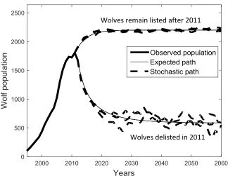
As shown in Figure 2, approximately 100 wolves were reintroduced in central Idaho and YNP in 1995 (𝑃0 = 101) and population growth in the region has begun to taper off around 2000 wolves. The population trend in Figure 2 suggests that wolf growth may be characterized by a logistic growth function. Periods of disease outbreak, perturbations in snow depth and prey availability introduced different degrees of
stochasticity into population dynamics (Coulson, et al. 2011;Smith, et al. 2011). Based on work suggesting that demographic stochasticity accounts for a greater percentage of variation in wolf growth rate than winter climate (Vucetich and Peterson 2004), we choose 𝜎(𝑃) =𝜎𝑃 such that the variation in wolf growth rate increases as the population declines. This formulation is consistent with Melbourne and Hastings (2008) which shows that increasing variance at low population levels is amplified by demographic heterogeneity. These assumptions allow us to rewrite equation (2) as
(12) 𝑑𝑃 = [𝑟𝑃 (1 −𝑃
𝐾) − ℎ(𝑃, 𝑆)𝑃] 𝑑𝑡 + 𝜎 𝑃𝑑𝑧
where r is the intrinsic growth rate of the population, 𝐾 is the carrying capacity of the population, and 𝜎 is a (constant) standard deviation coefficient. The expected value of the population grows at rate r when the population is small but growth gradually reduces to zero as the population approaches carrying capacity. The risk of extinction increases at low population levels since the variation in wolf growth rate is larger when P is small.
18
approximation of the density and its conditional moments, we transform equation (12) with h = 0 to a process with a constant diffusion term:
(13) 𝑑𝑌 = [𝑟2𝑌 (1 −√2𝑌 𝐾 ) +
𝜎2
4𝑌] 𝑑𝑡 + 𝜎𝑑𝑧
where 𝑌 = 𝑃2⁄2. The conditional transition density for a constant diffusion process is more Gaussian in nature which helps reduce approximation error (Bally and Talay 1996). We then employ a second-order Milstein approximation to equation (13). Compared to a first-order (Euler) approximation, the Milstein approximation increases the accuracy of our parameter estimates by considering the expansion of the non-constant drift term in equation 13 (Kloeden and Platen 1992). We use numerical quadrature, as opposed to Monte Carlo simulations, to reduce error associated with the numerical integration needed to compute the conditional transition density and ease the computational burden. The results are presented in Figure 2 and yield the following estimates: 𝑟 = 0.309,
𝜎 = 31,405, and 𝐾 = 2,198. To illustrate what these values imply about potential future outcomes, we performed 10,000 Monte Carlo simulations (each 50 years in duration) of the stochastic differential equation in equation (12). If the population were to remain listed after 2011 (h = 0), the population never went extinct in any of the simulations. Figure 3 shows the expected population and three Monte Carlo simulations.
http://www.fws.gov/mountain-19
prairie/species/mammals/wolf/), public harvest of wolves between 2012 and 2015 removed approximately 27% of the NRM wolf population.18 However, the rate of wolf removals can be expected to decline as the population declines. For example, Wyoming lowered harvest quotas between 2012 and 2013 which helped lower the rate of wolf removals from 24% to 21% (Wyoming Game and Fish Department 2013;Wyoming Game and Fish Department 2014). We consider an agency hunting rule that is consistent with NRM harvest rates between 2012 and 2015: ℎ = 0.27 − (1749 − 𝑃)𝑥 where 1749 is the average year-end wolf population between 2012 and 2015 and 0 ≤ 𝑥 ≤ 0.00015 captures the state agency response to declining wolf populations.19 Unfortunately, state agency response to declining wolf populations is unclear due to the limited time wolf hunting has been allowed. For exposition, we assume 𝑥 = 0.000035. A sensitivity analysis is undertaken to consider more or less responsive state management. To more clearly illustrate the impact of delisting, Figure 3 shows the expected population and three Monte Carlo simulations of equation (12) under the linear agency harvesting rule. Note that the volatility of the population increases as it declines capturing the increase in variance from demographic stochasticity and heterogeneity at low populations
(Melbourne and Hastings 2008). This makes extinction more likely when the population is delisted. Of the 10,000 50-year Monte Carlo simulations of the delisted population, gray wolves went extinct 664 times (6.6%). Average time to extinction was 37 years including simulations where extinction did not occur.
20
with a constant elasticity demand function 𝐵 = 𝛾𝑃𝑎 where 𝛾 > 0 is a scalar and the constant price elasticity is given by 𝑎−11 . Loomis and White (1996) report an average willingness to pay per wolf of $93 (2006$) in 1993 when there were 55 wolves in the northern Rocky Mountain region. Thirteen years later the population had grown to 1300 and Richardson and Loomis (2009) report an average willingness to pay per wolf of $61 (2006$). The two estimates represent points on a representative agent’s demand curve for gray wolves and suggest a constant price elasticity of -7.5 (𝑎 = 0.87).
In 2005, the gray wolf population in YNP was 118 and the annual direct expenditure impact associated with gray wolf presence in YNP was estimated at $35.5 million with a 95% confidence interval of $22.2 to 48.6 million (Duffield, et al. 2006). The 1994 Environmental Impact Statement (EIS) for gray wolf introduction estimated livestock losses from wolf predation and impacts on big game hunting at $16,200 and $325,500 respectively (U.S. Fish and Wildlife Service 1994).20 These studies suggest the annual net benefit of wolf presence in YNP in 2005 was $35.2 million with a standard deviation of $6.6 million.21 When evaluated at the mean, this implies
𝛾 = 35.2 118⁄ 0.87= 0.563.
There is also little information on the costs associated with endangered species listings and even less concerning delistings. Northern Rocky Mountain Wolf Recovery Reports provide an annual estimate of the amount spent at the federal level for
21
suggest that $2,000 to $3,000 dollars was spent per wolf. Of course federal expenditures serve as a lower bound estimate since they omit many private costs of species listing such as livestock losses that could not be tied to wolf predation, impacts to property values, effects on big game hunting, and lost hunter revenue. For exposition, we assume
𝑉(𝑃, 2) = 𝜈𝑃 with a variable cost of continued wolf listing of $50,000: v = 0.05.22 Delisting is assumed to cut these costs by 95%: 𝑉(𝑃, 3) = 𝑉(𝑃, 2)/20. We also assume the delisting and relisting costs are $45 million (𝐶𝐷 = 𝐶𝑅 = 45). By comparison, the total public transaction cost for listing the green sea turtle and loggerhead turtle was $154 million in 1991 dollars (Shogren and Hayward 1997). Boettiger, et al. (2015) suggest that underestimating these transaction costs has a consistently worse economic impact than overestimating them.
Bioeconomic thresholds for delisting and relisting
As expected, the approximated value function of the species when listed,
𝑊(𝑃, 2), and the approximated value function of the species when delisted, 𝑊(𝑃, 3), are increasing in P. The approximated state space extends from 0 to 2 in the 𝑃 𝐾⁄
dimension.23 Increasing the number of nodal points beyond 𝑛 = 200 or extending the state space does not alter our general results.
22
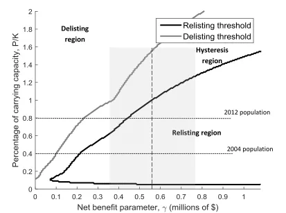
pair (𝛾, 𝑃/𝐾), is in the hysteresis region, no change should be made to the protected status of wolves. A smaller economic impact from wolves (leftward movement along the x-axis) or a sufficiently large increase in the population (upward movement along the y-axis) will trigger wolf delisting. This represents a switch from the no hunting to managed hunting regime. Once delisted, a larger economic impact from gray wolves (rightward movement along the x-axis) or a sufficiently large decrease in the wolf population (downward movement along the y-axis) will trigger relisting. This represents a switch from the delisted to the listed regime. Note that a declining gray wolf population will eventually be listed provided 𝛾 is more than $60,000.
Both curves are generally upward sloping from the origin. The exception is the lower boundary of the listing region. This region reflects those instances when the population of wolves is low enough that they are likely to go extinct. The chance of extinction in this region is so high that decision makers will not want to commit funds to listing wolves in our optimal switching framework as they are likely to go extinct even with federal protection. Here the threshold slopes down indicating a willingness to take a chance on a nearly extinct population that yields large economic impacts. This
willingness to keep the species off the endangered species list arises through the inclusion of the relisting option value.
23
our model does not treat 𝛾 as a random variable. However, the 95% confidence interval does indicate a likely range for the critical delisting and relisting thresholds. Delisting in 2012 could only be justified if 𝛾 is less than $240,000; a value outside the 95%
confidence interval. When NRM gray wolves were initially delisted in 2004, delisting was even more difficult to justify, and should have taken place only if 𝛾 was less than $100,000. Note that relisting could not be justified in 2012 if 𝛾 is less than $440,000. In other words, gray wolves no longer necessitate a spot on the endangered species list if the economic impact of gray wolf presence is in the lower end of the 95% confidence
interval. However, due to the decision making hysteresis created by the sunk costs associated with delisting, this argument against the relisting decision does not justify delisting.
The degree of gray wolf population recovery needed to justify delisting depends on the net benefit scalar. If 𝛾 lies at the lower end of the 95% confidence interval, populations would have to reach or exceed current estimates of carrying capacity in a single period. If 𝛾 lies at the upper end of the 95% confidence interval, populations would have to reach or exceed current estimates of carrying capacity by 90% in a single period. Out of 10,000 Monte Carlo simulations, the listed population never exceeded the carrying capacity by more than 2 percent. Justifying delisting is difficult due to the potential for regret. Because the payoffs from these decisions are uncertain and
24
Sensitivity analysis
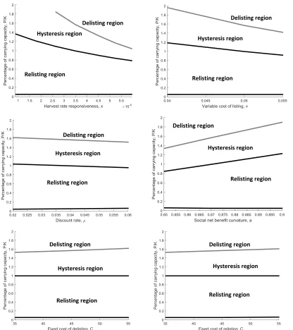
These results are dependent on our assumptions over the benchmark parameters. Figure 5 shows how changes in benchmark parameters impact the critical level of 𝑃/𝐾 that triggers delisting and relisting when the net benefit parameter is at its mean: 𝛾 =
0.563. An upward movement across the gray line triggers delisting while a downward movement across the upper black line triggers relisting (the lower black line is the lower bound of the relisting region). Small changes in discount rate and fixed cost have very little impact on our benchmark results. However, these results are sensitive to the responsiveness of state agency hunting management, the variable cost of listing, and the curvature of the social benefits function. Increasing the responsiveness of state agencies (x) and increasing the variable cost of listing (v) makes it harder to justify relisting but makes justifying delisting much easier. A perspective that views the endangered species listing as costly, and the repercussions of delisting as small, will be more inclined to support delisting. In contrast, more elastic demand for NRM gray wolves (a) makes it easier to justify relisting but harder to justify delisting.
25
that render those actions more costly also make subsequent decisions less likely. The more you fight a species listing, the larger the burden of proof required for delisting. If decision makers expect costly opposition to attempts to delist a species, listing becomes less likely.
The strength of this analysis is in its ability to incorporate stochastic changes in the wolf population. To determine the effect of future biological uncertainty at all population levels, Figure 6 compares the relisting and delisting thresholds with the benchmark level of uncertainty and no uncertainty. Biological uncertainty plays a bigger role at smaller populations making it more important in listing decisions. As shown by the shaded region in figure 6, uncertainty in future populations does imply slightly more precautionary behavior in that species should be listed sooner than they otherwise would. It also implies that a decision maker is less inclined to list an at-risk species at very low population levels where the probability of extinction is very high even if the species is protected. This motivation is captured by the hatched region in figure 6. Under our bioeconomic framework, a decision maker wishes to avoid making investments in species preservation that are unlikely to prevent extinction. This motivation may influence agency officials given limited budgets for listing and deslisting. Unfortunately, with demographic stochasticity, those species that are most at risk, also have the most uncertain future populations and represent the most risky investments in species conservation.
26
The bioeconomic decision thresholds in figures 4-6 carefully balance the risk of extinction with economic considerations. Based on this bioeconomic criterion, it is hard to justify the USFWS decision to delist the gray wolf in 2012. This is not surprising since the statutory language of the ESA prohibits the USFWS from using such a criterion. In the 2003 Federal Register Notice accompanying the original delisting, the USFWS indicated that the NRM gray wolf population was delisted in Montana and Idaho because 1) it exceeded numerical distributional and temporal goals and 2) state laws and wolf management plans were adequate to assure the USFWS that state shares of the NRM wolf population would be maintained above recovery levels. Recovery goals and state plans appear to have convinced the USFWS that the probability of gray wolf survival if delisted exceeded a minimum acceptable level.
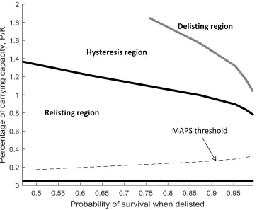
To compare our bioeconomic thresholds to a decision criterion more consistent with USFWS decisions, we follow Smith and Shogren (2001) and define a minimum acceptable probability of survival (MAPS). According to a MAPS decision criterion, a species should only be delisted if state level harvest plans (proxied in our model by x) are sufficient to ensure a minimum acceptable probability of survival.
27
long-run probability of wolf survival. A larger minimum acceptable probability of survival (rightward movement along the x-axis) would necessitate a higher minimum recovery goal and a higher population threshold needed to trigger delisting. For example, the USFWS originally delisted the gray wolf when it reached 40% of its carrying
capacity. If this decision were based on a MAPS, it would imply that USFWS deemed a less than 99% probability of survival as unacceptable. The bioeconomic thresholds are the solution to our regime switching model under different levels of x. Since each level of x implies a specific probability of wolf survival if delisted, we plot these bioeconomic thresholds with the equilibrium probability of survival on the x-axis. Much like the upper left panel in figure 5, a decision maker is more likely to delist and less likely to relist if the probability of survival when delisted is high.
Both the bioeconomic delisting and relisting thresholds are larger than the delisting threshold based on a MAPS criterion. The bioeconomic criterion recognizes that species recovery may be lower than expected following a sunk cost investment to delist the species. This gives regulators an incentive to delay delisting until the population far surpasses its recovery goal. The bioeconomic criterion also recognizes that relisting may be economically viable before a population falls below its recovery goals. Clearly, the decision to prohibit economic considerations in listing and delisting decisions was intended to avoid situations where regulators are moved to inaction
28
delisting) may actually afford greater protection for at-risk species if these decisions are initiated before the population drops out of the relisting threshold.
Conclusions
Opponents of the ESA have cited its lack of economic considerations in the listing decision as a fundamental flaw leading to unnecessary stakeholder conflicts and difficult species preservation goals for government agencies. Proponents cite the risk of
extinction and the inherent uncertainty concerning future populations as justification for the ESA’s “science only” mandate. This study speaks to both arguments by treating listing and delisting decisions as a linked set of risky investment options. As the first study to consider the optimal timing of delisting, this paper also informs the persistent debate over what constitutes a recovered population.
29
This hysteresis also makes it very difficult to justify delisting as species will be required to recover to levels that are likely to be much higher than historically observed. Since decision-making hysteresis is caused by the combination of sunk costs and
uncertainty, species with sizable upfront costs associated with delisting and a large amount of uncertainty in future population size will constitute a more difficult case for delisting. Here, economic considerations actually convey greater protections for
endangered species. This result also has implications for interest groups that may seek to influence listing and delisting decisions. Delisting becomes more difficult to justify when efforts to fight a species listing (e.g., litigation) make that decision more costly. Decision makers will be more inclined to delay delisting and avoid the possibility that species numbers will again dwindle and trigger another costly listing exercise. Listing decisions may also be delayed if decision makers anticipate a costly battle over delisting.
With increasingly tight budgets, safe investments in species conservation are preferred to risky ones, all other factors equal. A risky investment in species
conservation is one where substantial amounts of money are spent to list a species only to find out that the species is at less risk than previously thought due to a positive population shock or it went extinct in spite of the investment in protection. Of course, delaying listing also risks the species going extinct while these determinations are made. If future population levels are known with certainty, these considerations are eliminated.
30
population necessitates more immediate relisting. However, if the wolf population becomes too low, the potential for likely extinction can delay relisting investments. Thus, the species most in need of ESA protection will also represent the most risky investment of agency funds.
Most importantly, these results highlight the need to jointly consider listing and delisting decisions. The expected present value of increases in species benefits obtained by listing depends on how long a species is listed. This implies that the optimal timing of species listing is predicated on the subsequent delisting being optimally timed as well. Premature delisting decreases the expected benefits of species listing and calls into question the optimality of the initial listing decision. Failure to recognize this temporal relationship compromises both ecological objectives (species preservation) and economic objectives (maximizing net benefits from species conservation activities).
These results help explain persistent stakeholder conflicts that have plagued the ESA and also offer guidance for the future as the ESA celebrates its 40th anniversary. Our model represents a first step toward developing practical, quantitative criteria for listing and delisting decisions and the gray wolf example illustrates how population data and economic studies can be used to apply our methodology. However, there are a number of potential avenues for future work.
31
Possingham (2008) investigate the problem of managing harvests of a species for which the probability of recovery from a collapsed state is not known. Chadès et al. (2008) considers whether and when management of a rare species should switch from active management (anti-poaching activity) to monitoring and when preservation activities should be abandoned altogether. A number of studies have investigated harvesting when the size of the population is not perfectly observed (Clark and Kirkwood 1986;Moxnes 2003;Sethi, et al. 2005). Fackler and Pacifici (2014) discuss a model with both structural and observation uncertainty in a discrete time framework. Combining these various sources of uncertainty in an optimal switching model is a promising area of development. Since optimal switching models are typically developed in continuous time, and
continuous time models that include structural and observational uncertainty have not yet been developed, we leave this for future work.
Second, the current model considers sunk costs that can be avoided by delaying the decision to list or delist a species. Sunk costs may precede these decisions. For example, costly scientific studies and public hearings may be required before a listing or delisting decision is made. A more complete accounting for these timing considerations would treat research/outreach and listing/delisting as sequential or staged investments (Majd and Pindyck 1987). Listing/delisting would only be possible following the
32
choose to delay the actual listing decision. Such an approach would lower the option value associated listing and delisting but will not qualitatively change our results.
Third, our decision framework identifies the optimal timing of listing or delisting by comparing the rate of return from these actions across time. This is appropriate in situations where agency officials must determine whether a listing should be made within a predefined statutory timeline. However, it does not compare the rate of return for listing and delisting across species. A portfolio theory approach (Ando and Mallory 2012) may be more appropriate if the goal is to prioritize species for listing and delisting.
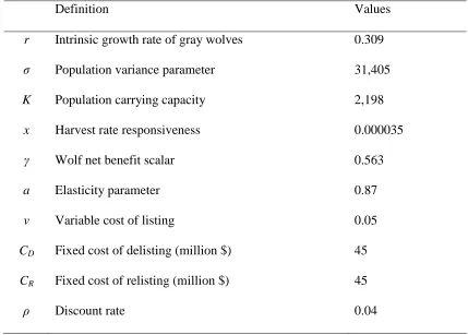
33 Table 1. Parameter Values and Definitions
Definition Values
r Intrinsic growth rate of gray wolves 0.309
σ Population variance parameter 31,405
K Population carrying capacity 2,198
x Harvest rate responsiveness 0.000035
γ Wolf net benefit scalar 0.563
a Elasticity parameter 0.87
v Variable cost of listing 0.05
CD Fixed cost of delisting (million $) 45
CR Fixed cost of relisting (million $) 45
34
35
36
Figure 3. Observed wolf population from 1995-2012, expected wolf population from 2012-2060, and stochastic wolf population paths based on estimates of r, σ, and K assuming wolves remain listed and are delisted in 2011.
37
Figure 4. Listing and delisting thresholds for gray wolves in Northern Rocky Mountain region with benchmark parameters presented in Table 1. The dashed line and gray shaded area represents mean and 95% confidence interval for γ based on a constant price elasticity of -7.5 and economic impacts from Duffield, et al. (2006) and the 1994 EIS.
Hysteresis region
Relisting region Delisting
region
2012 population
38
Figure 5. Sensitivity of listing and delisting thresholds to changes in benchmark parameters.
Hysteresis region Delisting region
Relisting region
Hysteresis region Delisting region
Relisting region Hysteresis region Delisting region
Relisting region Hysteresis region
Delisting region
Relisting region
Hysteresis region
Delisting region
Relisting region Relisting region
Hysteresis region
39
Figure 6. Impact of biological uncertainty on species delisting and relisting thresholds
σ = 31,405
40
Figure 7. Bioeconomic and minimum acceptable probability of survival (MAPS) decision criteria
Delisting region
Hysteresis region
Relisting region
41 References
Abdallah, S.B., and P. Lasserre. 2012. "A real option approach to the protection of a habitat dependent endangered species." Resource and Energy Economics 34:295-318.
Ando, A.W. 1999. "Waiting to Be Protected Under the Endangered Species Act: The Political Economy of Regulatory Delay." The Journal of Law and Economics
42:29-60.
Ando, A.W., and M.L. Mallory. 2012. "Optimal portfolio design to reduce climate-related conservation uncertainty in the Prairie Pothole Region." Proceedings of the National Academy of Sciences 109:6484-6489.
Balikcioglu, M., P.L. Fackler, and R.S. Pindyck. 2011. "Solving optimal timing problems in environmental economics." Resource and Energy Economics 33:761-768.
Bally, V., and D. Talay. 1996. "The law of the Euler scheme for stochastic differential equations: II. Convergence rate of the density." Monte Carlo Methods and Applications 2:93-128.
Bishop, R.C. 1978. "Endangered species and uncertainty: the economics of a safe minimum standard." American Journal of Agricultural Economics 60:10-18.
42
Brekke, K., and B. Øksendal. 1994. "Optimal Switching in an Economic Activity under Uncertainty." SIAM Journal on Control and Optimization 32:1021-1036.
Brown, G.M., and J.F. Shogren. 1998. "Economics of the endangered species act." The Journal of Economic Perspectives 12:3-20.
Bulte, E.H., and G.C. van Kooten. 2001. "Harvesting and conserving a species when numbers are low: population viability and gambler's ruin in bioeconomic models."
Ecological Economics 37:87-100.
Campbell, T., et al. 2015. "Protecting the Lesser Prairie Chicken Under the Endangered Species Act: A Problem and an Opportunity for the Oil and Gas Industry." Tex. Envtl. LJ 45:31.
Chadès, I., et al. 2008. "When to stop managing or surveying cryptic threatened species."
Proceedings of the National Academy of Sciences 105:13936-13940.
Clark, C.W. 1990. Mathematical Bioeconomics: Optimal Management of Renewable Resources. 2nd Ed. ed. Hoboken, New Jersey: John Wiley & Sons, Inc.
Clark, C.W., and G.P. Kirkwood. 1986. "On uncertain renewable resource stocks: optimal harvest policies and the value of stock surveys." Journal of
Environmental Economics and Management 13:235-244.
43
Courchamp, F., et al. 2006. "Rarity value and species extinction: the anthropogenic allee effect." PLoS Biology 4:e415.
Creel, S., and J.J. Rotella. 2010. "Meta-analysis of relationships between human offtake, total mortality and population dynamics of gray wolves (Canis lupus)." PLoS One
5:e12918.
Dixit, A. 1989. "Entry and Exit Decisions under Uncertainty." The Journal of Political Economy 97:620-638.
Doremus, H. 1997. "Listing decisions under the Endangered Species Act: why better science isn't always better policy." Wash. ULQ 75:1029.
Doremus, H., and J.E. Pagel. 2001. "Why Listing May Be Forever: Perspectives on Delisting under the U.S. Endangered Species Act." Conservation Biology
15:1258-1268.
Duffield, J., C. Neher, and D. Patterson. 2006. "Wolves and people in Yellowstone: Impacts on the regional economy." University of Montana, Final Report for Yellowstone Park Foundation.
Engen, S., and B.-E. Saether. 2000. "Predicting the time to quasi-extinction for populations far below their carrying capacity." Journal of Theoretical Biology
44
Fackler, P., and K. Pacifici. 2014. "Addressing structural and observational uncertainty in resource management." Journal of Environmental Management 133:27-36.
Fackler, P.L. 2013. "Structural and observational uncertainty in environmental and natural resource management." International Review of Environmental and Resource Economics 7:109-139.
Federal Register. 2010. Notice of Review: Endangered and Threatened Wildlife and Plants; Review of Native Species That Are Candidates for Listing as Endangerd
or Threatened; Annual Notice of Findings on Resubmitted Petitions; Annual
Description of Progress on Listing Actions, Vol. 75(217). Rep. 50 CFR Part 17.
Fisher, A.C. 2000. "Investment under uncertainty and option value in environmental economics." Resource and Energy Economics 22:197-204.
Geske, R. 1979. "The valuation of compound options." Journal of Financial Economics
7:63-81.
Ginzburg, L.R., et al. 1982. "Quasiextinction probabilities as a measure of impact on population growth." Risk Analysis 2:171-181.
Goble, D.D. 2009. "The Endangered Species Act: What we talk about when we talk about recovery." Natural Resources Journal 49:1-44.
45
Gude, J.A., et al. 2012. "Wolf population dynamics in the US Northern Rocky Mountains are affected by recruitment and human‐caused mortality." The Journal of
Wildlife Management 76:108-118.
Hauser, C.E., and H.P. Possingham. 2008. "Experimental or precautionary? Adaptive management over a range of time horizons." Journal of Applied Ecology 45:72-81.
Innes, R., S. Polasky, and J. Tschirhart. 1998. "Takings, compensation and endangered species protection on private lands." The Journal of Economic Perspectives :35-52.
Judd, K. 1998. Numerical Methods in Economics: MIT Press.
Kassar, I., and P. Lasserre. 2004. "Species preservation and biodiversity value: a real options approach." Journal of Environmental Economics and Management
48:857-879.
Kloeden, P.E., and E. Platen. 1992. Numerical Solution of Stochastic Differential Equations: Springer.
46
Leroux, A.D., V.L. Martin, and T. Goeschl. 2009. "Optimal conservation, extinction debt, and the augmented quasi-option value." Journal of Environmental Economics and Management 58:43-57.
Loomes, G., and R. Sugden. 1982. "Regret theory: An alternative theory of rational choice under uncertainty." The Economic Journal:805-824.
Loomis, J.B., and D.S. White. 1996. "Economic benefits of rare and endangered species: summary and meta-analysis." Ecological Economics 18:197-206.
Majd, S., and R.S. Pindyck. 1987. "Time to Build, Option Value, and Investment Decisions." Journal of Financial Economics 18:22.
Marten, A.L., and C.C. Moore. 2011. "An options based bioeconomic model for biological and chemical control of invasive species." Ecological Economics
70:2050-2061.
Meek, M.H., et al. 2015. "Fear of failure in conservation: The problem and potential solutions to aid conservation of extremely small populations." Biological Conservation 184:209-217.
Melbourne, B.A., and A. Hastings. 2008. "Extinction risk depends strongly on factors contributing to stochasticity." Nature 454:100-103.
47
Morgan, D.G., S.B. Abdallah, and P. Lasserre. 2007. "A real options approach to forest-management decision making to protect caribou under the threat of extinction."
Ecology and Society 13:27.
Moxnes, E. 2003. "Uncertain measurements of renewable resources: approximations, harvesting policies and value of accuracy." Journal of Environmental Economics and Management 45:85-108.
Neel, M.C., et al. 2012. "By the numbers: How is recovery defined by the US endangered species act?" BioScience 62:646-657.
Nøstbakken, L. 2006. "Regime switching in a fishery with stochastic stock and price."
Journal of Environmental Economics and Management 51:231-241.
NRC. "Science and the Endangered Species Act." National Research Council (US). Committee on Scientific Issues in the Endangered Species Act.
Olsen, J.R., and J.S. Shortle. 1996. "The optimal control of emissions and renewable resource harvesting under uncertainty." Environmental and Resource Economics
7:97-115.
Pindyck, R.S. 2007. "Uncertainty in Environmental Economics." Review of Environmental Economics and Policy 1:45-65.
48
Prato, T. 2005. "Accounting for uncertainty in making species protection decisions."
Conservation Biology 19:806-814.
Qi, H., and L. Liao. 1999. "A Smoothing Newton Method for Extended Vertical Linear Complementarity Problems." SIAM Journal on Matrix Analysis and Applications
21:45-66.
Ready, R.C., and R.C. Bishop. 1991. "Endangered species and the safe minimum standard." American Journal of Agricultural Economics 73:309-312.
Regan, T.J., et al. 2013. "Testing Decision Rules for Categorizing Species’ Extinction Risk to Help Develop Quantitative Listing Criteria for the U.S. Endangered Species Act." Conservation Biology 27:821-831.
Richardson, L., and J. Loomis. 2009. "The total economic value of threatened,
endangered and rare species: An updated meta-analysis." Ecological Economics
68:1535-1548.
Robbins, K. 2009. "Strength in numbers: setting quantitative criteria for listing species under the Endangered Species Act." UCLA Journal of Environmental Law & Policy 27:2.
49
Salau, K.R., and E.P. Fenichel. 2014. "Bioeconomic analysis supports the endangered species act." Journal of Mathematical Biology:1-30.
Sethi, G., et al. 2005. "Fishery management under multiple uncertainty." Journal of Environmental Economics and Management 50:300-318.
Shogren, J.F., and P.H. Hayward. 1997. "Biological effectiveness and economic impacts of the Endangered Species Act." Land & Water L. Rev. 32:531.
Shogren, J.F., et al. 2001. "Why economics matters for endangered species protection."
Conservation Biology 13:1257-1261.
Smith, D., et al. "Yellowstone Wolf Project: Annual Report, 2010." National Park Service, Yellowstone National Park, Yellowstone Center for Resources.
Smith, R.B., and J.F. Shogren (2001) "Protecting species on private land." In Protecting Endangered Species in the United States: Biological Needs, Political Realities,
and Economic Choices. Cambridge, Cambridge University Press, pp. 326-343.
Song, F., J. Zhao, and S.M. Swinton. 2011. "Switching to Perennial Energy Crops Under Uncertainty and Costly Reversibility." American Journal of Agricultural
Economics 93:768-783.
50
Tear, T.H., et al. 2005. "How much is enough? The recurrent problem of setting measurable objectives in conservation." BioScience 55:835-849.
Trigeorgis, L. 1996. Real Options: Managerial Flexibility and Strategy in Resource Allocation. Cambridge, Massachusetts: The MIT Press.
U.S. Fish and Wildlife Service. "The reintroduction of gray wolves to Yellowstone National Park and central Idaho. Final Environmental Impact Statement.".
U.S. Fish and Wildlife Service, Idaho Department of Fish and Game, Montana Fish, Wildlife & Parks, Nez Perce Tribe, National Park Service, Blackfeet Nation, Confederated Salish and Kootenai Tribes, Wind River Tribes, Confederate Colville Trbies, Washington Department of Fish and Wildlife, Oregon
Department of Fish and Wildlife, Utah Department of Natural Resources, and USDA Wildlife Services. 2013. Northern Rocky Mountain Wolf Recovery Program 2012 Interagency Annual Report, eds. M.D. Jimenez and S.A. Becker.
USFWS, Ecological Services, 585 Shepard Way, Helena, Montana, 59601.
51
2011, eds. M.D. Jimenez and S.A. Becker USFWS, Ecological Services, 585 Shepard Way, Helena, Montana, 59601.
U.S. Fish and Wildlife Service, Nez Perce Tribe, National Park Service, and USDA Wildlife Services. 2004. Rocky Mountain Wolf Recovery 2003 Annual Report, eds. T Meier. USFWS, Ecological Services, 100 N Park, Suite 320, Helena, MT. 65 pp.
van der Heide, C.M., J.C. van den Bergh, and E.C. van Ierland. 2005. "Extending Weitzman's economic ranking of biodiversity protection: combining ecological and genetic considerations." Ecological Economics 55:218-223.
van Kooten, G.C., and E.H. Bulte. 2000. The Economics of Nature: Managing Biological Assets: Blackwell Oxford.
Varley, N., and M.S. Boyce. 2006. "Adaptive management for reintroductions: updating a wolf recovery model for Yellowstone National Park." Ecological Modelling
193:315-339.
Vucetich, J.A., and R.O. Peterson. 2004. "The influence of prey consumption and
demographic stochasticity on population growth rate of Isle Royale wolves Canis lupus." Oikos 107:309-320.
52
---. 1993. "What to preserve? An application of diversity theory to crane conservation."
The Quarterly Journal of Economics:157-183.
Willassen, Y. 1998. "The stochastic rotation problem: A generalization of Faustmann's formula to stochastic forest growth." Journal of Economic Dynamics and Control
22:573-596.
Wilson, M.A. 1997. "The wolf in Yellowstone: Science, symbol, or politics?
Deconstructing the conflict between environmentalism and wise use." Society & Natural Resources 10:453-468.
Wines, M. (2013) "Endangered or Not, but at Least No Longer Waiting." In The New York Times.
Woods, T., and S. Morey. 2008. "Uncertainty and the Endangered Species Act." Ind. LJ
83:529.
Wyoming Game and Fish Department, U.S. Fish and Wildlife Service, National Park Service, USDA-APHIS-Wildlife Services, and Eastern Shoshone and Northern Arapahoe Tribal Fish and Game Department. 2013. 2012 Wyoming Gray Wolf Population Monitoring and Management Annual Report. eds. K.J. Mills and R.F.
53
---. 2014. 2013 Wyoming Gray Wolf Population Monitoring and Management Annual Report. eds. K.J. Mills and R.F. Trebelcock Wyoming Game and Fish
54 Footnotes
1 Our usage of the term “regret” is narrow and in line with the option value literature. This concept of regret originates from a dynamic framework where a decision today limits decisions in the future and new information is revealed over time. In this setting, the status quo influences optimal ex post decisions (Dixit 1989). In contrast, the regret theory of Loomes and Sugden (1982) is a static concept of regret where a reference point is explicitly included in the decision maker’s utility function.
2The ESA outlines statutory timelines to propose a listing (Woods and Morey 2008). This restriction creates a decision window that limits decision makers from being able to capture the entire option value associated with listing. However, extensions are common and in some cases extend for decades (Wines 2013). In contrast, delisting is a far more flexible process. Our alternative decision framework allows federal agency decision makers to fully capture the listing and delisting option value.
3 For general applications of real options methodology to a single species conservation investment see Morgan et al. (2007), Kassar and Lasserre (2004), Leroux et al. (2009), and Abdallah and Lasserre (2012). A compound option approach has been used to determine the optimal timber harvest strategy with
stochastic forest growth (Willassen 1998), entry and exit in a fishery with stochastic fish stock and price (Nøstbakken 2006), and crop conversion with uncertain returns (Song, et al. 2011).
4 This view was supported by the Supreme Court in the 1978 case, Tennessee Valley Authority v. Hill (437 U.S. 187, 184 (1978)). Amendments to the ESA in 1978 allowed economic considerations when
designating critical habitat.
5 In Animal Welfare Institute v. Beech Ridge Energy L.L.C., a conservation group successfully prevented the operation of a wind project in West Virginia due to impacts to the endangered Indiana bat (Ruhl 2012). Development of drilling infrastructure in the Permian Basin, a major oil and gas producing region in west Texas, is expected to decrease suitable habitat for the Lesser Prairie Chicken which was listed as
55
6 Funding for listing actions is determined through the annual Congressional appropriations process. In every fiscal year since 1998, Congress has placed a statutory cap on funds which may be expended on the ESA’s Listing Program (Federal Register 2010).
7 See Endangered Species Act Section 4 Deadline Litigation, No. 1:10-mc-377 (D.D.C., Sept. 9, 2011). 8 This paper focuses on biological uncertainty related to stochastic influences. Biological uncertainty may also arise through structural uncertainty and observational (state) uncertainty (Fackler and Pacifici 2014). We discuss the potential challenges associated with including these other sources of uncertainty in the concluding section of the paper.
9 This data was retrieved from the U.S. Fish and Wildlife Service’s Environmental Conservation Online System (ECOS) and do not include species that were delisted due to extinction.
10
The General Accounting Office reported that the total public transaction cost for thirty-four different species is approximately $700 million ranging from a 1994 cost of $145,000 for the White River spinedace to a 1991 estimate of $154 million for the green sea turtle and loggerhead turtle (Shogren and Hayward 1997). The median cost of preparing and publishing various listing documents alone is $39,276 for a 90-day finding, $100,690 for a 12-month finding, $345,000 for a proposed rule with critical habitat, and $305,000 for a final listing rule with critical habitat (Federal Register 2010).
11
An anthropogenic Allee effect suggests that a rarity value may encourage human activities that push species to extinction. For example, the value of being able to hunt a black rhinoceros may increase as the species becomes more endangered. This is in contrast to stock effects that suggest that extinction is less likely as populations decline due to the increasing costs of finding the last individuals.
12
The assumption that P(t) is perfectly observed at time t may fit some species better than others. A number of studies have investigated harvesting when the size of the population is not perfectly observed (Clark and Kirkwood 1986;Moxnes 2003;Sethi, et al. 2005). For a review of this literature see Fackler (2013).
13
56
other areas. Since reintroduction efforts require significant sunk costs, the optimal switching model described in this paper could be reinterpreted to investigate the optimal timing of this reintroduction. 14 Note that this differs from what the law requires regarding listing and delisting decisions. The model is similar to the entry and exit model of Dixit (1989) where market entry and exit is akin to species listing and delisting.
15 In some cases, the primary motivation for species listing is to protect large swaths of habitat and not necessarily to protect a specific species. In these cases, habitat metrics become the primary indicator of endangered and recovered status. These habitat preservation motivations can be accommodated by incorporating habitat metrics into the decision maker’s instantaneous returns.
16 For example, the Bonneville Power Administration estimated that its expenditure on salmon conservation was about $350 million in 1994, of which about $300 million represented an opportunity cost of lost power revenues (NRC 1995).
17
By backward induction, we solve the listing/delisting problem (conditions 8-11) before the optimal stopping problem (conditions 6-7).
18
Other sources of human-caused mortality (accidental killing, agency control) were present before the delisting decision and will be captured by the error term in equation (12). For more information on human-induced mortality on gray wolf populations in the area see Creel and Rotella (2010) and Gude et al. (2012). 19𝑥 ≤ 0.00015 ensures the harvest rate remains non-negative. We also considered a nonlinear agency hunting rule (ℎ = 0.0065√𝑃) which produces qualitatively similar results.
20 Varley and Boyce (2006) largely confirm the original 1994 EIS estimates of impacts on big game hunting.
21 This estimate of annual net benefit of gray wolf presence omits nonuse value for gray wolf presence in the NRM and should be interpreted as a lower bound. Nonuse values for species preservation are
57
22 Due to the lack of data on private costs of gray wolf listing, a sensitivity analysis is conducted on v. For instance, while wolf tags are currently sold in Idaho and Montana (were sold in Wyoming), they are relatively inexpensive and likely undervalue the economic impact of forgone hunting activity. We also consider nonlinear management cost functions which produce qualitatively similar results.
23 Solver efficiency and accuracy is significantly reduced when the approximated state space is large (Miranda and Fackler 2002). To bring the dimension of the approximated state space closer to unity, we scaled the problem by introducing the new variable 𝑁(𝑡) = 𝑃(𝑡) 𝐾⁄ with 𝑑𝑁 = 𝑟𝑁(1 − 𝑁)𝑑𝑡 + 𝜎
𝑁𝐾2𝑑𝑧.