https://doi.org/10.5194/gmd-10-4187-2017 © Author(s) 2017. This work is distributed under the Creative Commons Attribution 3.0 License.
Numerical framework for the computation of urban flux footprints
employing large-eddy simulation and Lagrangian
stochastic modeling
Mikko Auvinen1,2, Leena Järvi1, Antti Hellsten2, Üllar Rannik1, and Timo Vesala1,3
1Department of Physics, P.O. Box 64, University of Helsinki, 00014 Helsinki, Finland 2Finnish Meteorological Institute, P.O. Box 503, 00101 Helsinki, Finland
3Department Forest Sciences, P.O. Box 27, University of Helsinki, 00014 Helsinki, Finland
Correspondence to:Mikko Auvinen ([email protected]) Received: 9 December 2016 – Discussion started: 4 January 2017
Revised: 14 September 2017 – Accepted: 21 September 2017 – Published: 17 November 2017
Abstract.Conventional footprint models cannot account for the heterogeneity of the urban landscape imposing a pro-nounced uncertainty on the spatial interpretation of eddy-covariance (EC) flux measurements in urban studies. This work introduces a computational methodology that enables the generation of detailed footprints in arbitrarily complex urban flux measurements sites. The methodology is based on conducting high-resolution large-eddy simulation (LES) and Lagrangian stochastic (LS) particle analysis on a model that features a detailed topographic description of a real ur-ban environment. The approach utilizes an arbitrarily sized target volume set around the sensor in the LES domain, to collect a dataset of LS particles which are seeded from the potential source area of the measurement and captured at the sensor site. The urban footprint is generated from this dataset through a piecewise postprocessing procedure, which divides the footprint evaluation into multiple independent processes that each yield an intermediate result. These results are ul-timately selectively combined to produce the final footprint. The strategy reduces the computational cost of the LES–LS simulation and incorporates techniques to account for the complications that arise when the EC sensor is mounted on a building instead of a conventional flux tower. The presented computational framework also introduces a result assessment strategy which utilizes the obtained urban footprint together with a detailed land cover type dataset to estimate the po-tential error that may arise if analytically derived footprint models were employed instead. The methodology is demon-strated with a case study that concentrates on generating the footprint for a building-mounted EC measurement station in
downtown Helsinki, Finland, under the neutrally stratified at-mospheric boundary layer.
1 Introduction
Micrometeorological measurements in densely built city en-vironments pose an antipodal problem: they are essential in establishing the fundamental basis for the study of urban mi-croclimates, but these measurements are endowed with pro-nounced uncertainties, which mainly originate from the to-pographic and elemental complexity of the urban landscape. The resulting noncompliance between the theory and prac-tice in urban micrometeorological measurements undermines the study of how our cities interact with the surrounding at-mosphere. At the very heart of this discord lies the prob-lem concerning the determination of effective source areas, or footprints, of urban flux or concentration measurements.
η(xM)=
Z
f (xM,x0) Q(x0)dx0, (1)
where f has dimensions of inverse of integration units (m−3). In the subsequent presentation the vertical dimension of domain is collapsed and therebyf has dimensions of inverse area (m−2). The footprint can also be interpreted as a spatial weighting function that expresses the probability with which a fluid element that coincides with an element ofQ contributes to the measurement at xM (Pasquill and Smith, 1983). In accordance with Sogachev et al. (2005), this study does not adhere to the strict interpretation where the foot-print is only a function of turbulent diffusion and source-sensor location, but allows the possibility that, for instance, variations in source-area topography can influence the result. In this context, topography refers to an elevation model of the landand buildingstogether. Consequently, the footprint should provide the critical link between the point measure-ment and the geographical distribution of sources, yielding a complete characterization ofηwith regard to its contents. In an effort to achieve this, analytical closed-form solutions have been derived for the footprint functions – see Schmid (2002) for a comprehensive review – but only under the as-sumptions that (1) steady-state conditions prevail during the analyzed period, (2) turbulent fluctuations in the atmospheric boundary layer (ABL) are horizontally homogeneous, and (3) there is no vertical advection. These assumptions allow the governing equations to be reduced to a time-averaged balance between advection and turbulent diffusion which ad-mits, with appropriate parametrization of the turbulent flow field, a closed-form expression for the footprint function.
The underlying assumptions are often acceptable in mea-surement sites where the sensors are mounted on towers that have been appropriately placed above homogeneous forested landscapes and well above the surface roughness sublayer height where the effects of the individual roughness elements disappear. However, due to practical regulations constraining measurement campaigns in densely populated cities, suffi-ciently tall flux towers cannot be erected above the skyline of central urban areas. It is often inevitable that if the urban mi-croclimate is to be studied experimentally, the measurements must be obtained near the border of the roughness sublayer by sensors that are mounted either on low-rise towers or on top of tall buildings. In these suboptimal conditions, assump-tion (2) becomes strictly invalid and assumpassump-tion (3) highly questionable because urban boundary layer (UBL) flows are typically characterized by developing and strongly heteroge-neous flow conditions, particularly at lower elevations where individual buildings influence the turbulence.
Considering that the analytical footprint models effec-tively provide ellipse-shaped probability distributions for the source contributions without any regard to topographic het-erogeneities, it becomes clear that the use of such
source-area models becomes highly suspect in real urban conditions. This is an unacceptable state of affairs in the urban microm-eteorology research and immediately calls for targeted ef-forts to alleviate the uncertainties associated with the invalu-able urban flux-measurement data. Although, the first efforts by Vesala et al. (2008), utilizing the method by Sogachev et al. (2002), already explored topography-sensitive urban footprints, the applicability of the documented approach has not reached the scale and accuracy requirement of the urban footprint problems considered herein.
As a response, this works introduces a new numerical methodology to construct detailed topography-sensitive foot-prints for complex urban flux measurement sites by the means of pre- and postprocessing developments and a large-eddy simulation (LES) solver suite that features an embed-ded Lagrangian stochastic (LS) particle model. This coupled model will be referred to with the acronym LES–LS. The proposed methodology is designed to be first and foremost a postprocessing procedure, which exploits the current state-of-the-art LES–LS modeling framework in an urban setting with a minimal investment in the initial setup.
The principal objective is to provide a reliable compu-tational framework, founded on a high-resolution LES–LS analysis, to generate the most accurate footprint estimates feasible without the need to conduct tracer gas experiments, which are nearly impossible to arrange in residential areas. These computationally generated footprints open up the pos-sibility to study the appropriate placement of new measure-ment stations and to assess the magnitude of the potential misinterpretation which may arise from the application of closed-form footprint models to urban flux or concentra-tion measurements. The proposed framework is also supple-mented by a convenient technique to approximate this error with the assistance of a land cover classification dataset.
The methodology is demonstrated with a numerical case study, which is staged in Helsinki, the coastal capital city of Finland, and focuses on the eddy-covariance (EC) mea-surement site mounted on the roof of Hotel Torni (Nordbo et al., 2015; Kurppa et al., 2015), which is the tallest acces-sible building in the downtown region. The building height is 57.7 m and the EC sensor is situated 2.3 m above it corre-sponding to 74 m height above the sea level. Thus, the effec-tive measurement height (a.g.l) iszM=60 m –d=45.1 m, whered=14.9 m is the displacement height of the site ac-cording to Nordbo et al. (2013). The mean building height of the surrounding area is 24 m. The site belongs to SMEAR III (Station for Measuring Ecosystem–Atmosphere Relations, Järvi et al., 2009) and is also part of the urban network of atmospheric measurement sites (Wood et al., 2013). Its po-tential source area closely resembles a typical European city arrangement that features perimeter blocks with inner court-yards.
et al. (2008) and very recently by Hellsten et al. (2015), who constructed footprints for an idealized city environment as a precursor study to this work. The presented contribution places special emphasis on the issue of composing footprints for flux measurement sites that are surrounded by arbitrar-ily heterogeneous topography and may be compromised by the fact that they are mounted on top of actual buildings in-stead of conventional radio-mast-like towers. Such a com-plex urban setting requires a new mechanism for construct-ing footprints, which is accompanied by a requirement that the associated LES–LS simulation is capable of resolving the relevant turbulent structures ranging from the street-canyon-scale phenomena within the roughness sublayer to the larger ABL structures, while also accounting for the interaction be-tween them (Anderson, 2016).
2 Materials and methods
2.1 Numerical modeling framework
The PALM model utilized in this study is an open-source nu-merical solver for atmospheric and oceanic flow simulations. The software has been carefully designed to run efficiently on massively parallel supercomputer architectures and it is therefore exceptionally well suited for high-resolution UBL simulations considered herein. The LES model employs finite-difference discretization on staggered Cartesian grid and utilizes an explicit Runge–Kutta time-stepping scheme to solve the evolution of velocity vectoru=(u, v, w), mod-ified perturbation pressure π∗, potential temperatureθ, and specific humidityqv fields from the conservation equations for momentum, mass, energy, and moisture, respectively. The conservation equations are implemented in an incompress-ible, Boussinesq-approximated, non-hydrostatic, and spa-tially filtered form, which indicates that the conservation of mass is imposed by the solution to a Poisson equation forπ∗. The filtering refers to the separation of scales in LES where the turbulent scales containing the majority of energy are re-solved by the grid while the diffusive effect of the unrere-solved subgrid-scale (SGS) turbulence is accounted for by a SGS turbulence model. To achieve closure in the final system of equations, PALM implements the 1.5-order SGS turbulence model by Deardorff (1980), modified according to Moeng and Wyngaard (1988) and Saiki et al. (2000). The model in-volves an additional prognostic equation for SGS turbulent kinetic energy (SGS-TKE)e.
The embedded Lagrangian particle model in PALM imple-ments the time-accurate evolution of discrete particles (either with or without mass) through a technique that conforms to the LES approach: the trajectories are integrated in time such that the transporting velocity field is decomposed into de-terministic (i.e., resolved) and stochastic (i.e., subgrid-scale) contributions. The deterministic velocity components are di-rectly obtained from the LES solution, while the random
components are evaluated according to Weil et al. (2004). Although LS modeling approaches that are less computation-ally expensive exist (Glazunov et al., 2016), warranting fur-ther investigation on their applicability to urban problems, the presented high-resolution urban flow problem is assumed to require the highest level of description also from the LS model; the interaction between the atmospheric wind and the cascade of multistoried buildings and street canyons gives rise to strongly anisotropic turbulence structures, which are not reliably amendable to parametrization.
While the LES–LS simulations are carried out in large su-percomputing facilities, the preprocessing of the urban to-pography model and the postprocessing of the final footprint from raw data is performed on a personal workstation utiliz-ing freely available numerical scriptutiliz-ing and data visualiza-tion technologies. See the paragraph on code availability at the end of this paper.
2.2 Urban LES setup and analysis 2.2.1 Urban topography model
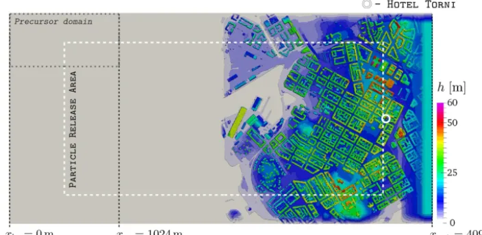
The urban topography model, used in describing the bottom wall boundary of the LES domain, is prepared from a de-tailed 2 m resolution laser-scanned dataset of the Helsinki area (Nordbo et al., 2015). The data are conveniently avail-able in raster map format and, in addition to the height distri-butionh(x, y), also include a distribution of land cover types LC(x, y)∈ {1,2, . . ., NLC}whereNLCis the number of land cover classes in the dataset. Both raster maps are shown in Fig. 1. Access to similar surface data source is a critical pre-requisite for the presented methodology.
The horizontal domain for the LES analysis extendsLx= 4096 m in the mean wind direction andLy=2048 m in the crosswind direction and is spatially oriented such thatxaxis is coincident with the geostrophic wind direction of the case study. The EC measurement site at Hotel Torni is pivotally located in the LES domain to facilitate the determination of its footprint. However, the extracted raster map has to be first purposefully preprocessed to attain a form that complies with the LES analysis-specific requirements. The following ma-nipulations were applied to obtain the final topography model depicted in Fig. 2.
1. The first half of the topography model (where x < Lx/2) is flattened for the purpose of generating phys-ically realistic ABL conditions at the inlet through tur-bulence recycling technique (see below).
2. The lateral sides were made identical for cyclic bound-ary condition treatment by applying a zero-height mar-gin that smoothly blends toward the values in the inte-rior.
Figure 1.Raster maps of topography heighth(a)and land cover typesLC(b)from Helsinki area. The rectangle in the bottom left corner is aligned with southwesterly wind and represents the area of interest for the footprint analysis. In the surface type classification each pixel (2 m) is categorized according to the following numbering: 0=building, 1=impervious (rock, paved, gravel), 2=grass, 3=low vegetation, 4=high vegetation, and 5=water.
turbulent flow (caused by the buildings near the end of the domain) to slightly accelerate before reaching the outlet boundary where reversed flow causes numerical difficulties.
2.2.2 Physical setup for the LES model
The meteorological conditions for the simulation are adopted from 9 September in 2012 when near-neutral ABL conditions were recorded with the EC measurements made on top of the Torni building. Lidar measurements (Wood et al., 2013) from the chosen time frame yielded|ug| =10 m s−1for the
geostrophic wind in a southwesterly direction (α=218◦) and δ≈300 m for the boundary layer height. The Coriolis force (corresponding to latitude 60◦N) is included to ac-count for the turning of the flow within the boundary layer. The meteorological conditions are conveyed to the simula-tion by means of a precomputed ABL solusimula-tion over flat sur-face, which in this context represents the surface of the Baltic Sea bordering Helsinki from the south. The boundary condi-tions for the velocity solution in this precursor simulation were set such that a fixed value is applied at the top and a no-slip condition at the bottom boundary of the domain while setting all the lateral boundaries as periodic.
For the precursor simulation the solver was run with an op-tion that explicitly conserves the initial mass flow rate across the system, which was specified by initializing the velocity field with a constant value ut=0=0.95ug. This
initializa-tion value was determined by trial and error with the objec-tive that the precursor solution would ultimately yield the de-sired geostrophic wind value atz=δfor the horizontally av-eraged velocity fieldh ¯uipre. The boundary layer growth was controlled by initializing the potential temperature field with a vertical profileθ0(z)that features a strong inversion layer
at 300< z <350 m. Thisθ0(z)profile is defined according
to the following lapse rates:
∂θ0
∂z =
0 K km−1 0 m≤z <300 m 50 K km−1 300 m≤z <350 m 3 K km−1 350 m≤z .
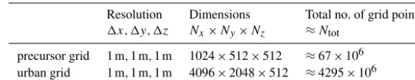
The precursor LES solution was computed on a grid that has the same resolution and vertical dimension as the princi-pal urban LES grid, but its lateral dimensions are smaller by an integer division. Table 1 summarizes the respective grid characteristics. The study features a spatial resolution of 1 m, which is unprecedented at this scale. Giometto et al. (2016) found the same resolution to be sufficient to capture the rel-evant turbulence physics within a real urban roughness sub-layer. However, the effect of grid resolution on the final result is not investigated in this work. The influence of the struc-tural details of the urban surface (balconies, chimneys, venti-lation ducts, stationary cars, small-scale vegetation, etc.) not included in the urban topography model are taken into ac-count by specifying a uniform roughness lengthz0=0.05 m
Figure 2.Visualization of the topography height distribution underlying the LES domain. The particle release area is enveloped by a white dashed line. The size of the precursor domain is outlined in the top left corner. The location of the turbulence recycling plane is marked by a black dotted line atxrc.
The precursor simulation generates a highly resolved ABL solution that will be utilized, first, in a recursive manner to initialize the entire urban LES flow field with turbulence and, second, to aid construction of appropriate inlet boundary conditions though a technique labeledturbulence recycling, which is based on the method by Lund et al. (1998) with modifications by Kataoka and Mizuno (2002). The imple-mentation of this boundary condition in PALM is presented in Maronga et al. (2015), but to aid discussion the description is also covered here with modified notation.
Denoting prognostic field variables byψ=ψ (x, t )where ψ∈ {u, v, w, θ, e}, the precursor solution is used to extract horizontally averaged vertical profiles¯
ψpre
(z) for the tur-bulence recycling boundary condition. These stationary pro-files are utilized at the inlet boundary in the urban simulation to conserve the global state of the mean flow, but in a manner that also incorporates physically sound turbulent fluctuations that occur in an ABL flow. This is achieved by specifying a recycling plane, that is, ayzplane at a windwise coordinate xrc, placed sufficiently far downstream from the inlet to
pre-vent feedback of disturbances between the two planes. The fluctuations are obtained from the recycling plane through the following technique:
ψ0
x=xrc
=ψ
x=xrc
− hψiy
x=xrc, (2)
where the spatial mean (in the crosswind direction)hψiy= hψiy(z, t ) at the recycling plane is computed as a time de-pendent vertical profile
hψiy
x=xrc=
1 Ny
Ny
X
i=1
ψ (xrc, yi, z, t ) (3)
that carries a dependence onNy. Finally, utilizing the pre-cursor generated mean profiles, the turbulence recycling inlet
boundary condition becomes ψx=x
in
=ψ¯pre+ψ0x=x
rc. (4)
In association with the turbulence recycling, the top bound-ary condition in the main simulation is specified as a slip-wall.
In this study, the recycling plane is situated, as shown in Fig. 2, in accordance with the precursor domain length such that(xrc−xin)=1024 m≈3.4δand the same distance is
al-located from the recycling plane to the edge of the urban to-pography to ensure that disturbances originating from the ur-ban terrain are not conveyed back to the inlet. The chosen tur-bulent inlet arrangement generated no observable feedback effect on the incoming turbulence field.
2.2.3 LS particle model setup for the footprint evaluation
The embedded LS particle model is employed such that, after the initial transients in the LES solution have subdued (after approximately 5 min of simulation), the release of particles is activated within the region outlined in Fig. 2. The release area extends 3030 m (≈41zM) in the upwind direction and 780 m (≈10.5zM) in both lateral directions from the Hotel Torni’s EC site. The release area has been trimmed accord-ing to preliminary trial simulations to reduce the number of redundant particles in the domain.
Denoting the Lagrangian coordinate vector of thelth par-ticle byXl(t )= Xl(t ), Yl(t ), Zl(t )
, the release locations
Xlo=Xl
t=0are uniformly distributed 2 m apart in thexand
Table 1.Computational grid specifications.
Resolution Dimensions Total no. of grid points 1x, 1y, 1z Nx×Ny×Nz ≈Ntot
precursor grid 1 m,1 m,1 m 1024×512×512 ≈67×106 urban grid 1 m,1 m,1 m 4096×2048×512 ≈4295×106
It also lowers the risk of accumulating a large number of particles within the first grid cell where the velocity values are dictated by the logarithmic wall function and the vertical advection of particles solely by the stochastic model due to Weil et al. (2004). Thus, the underlying assumption is that, at 1 m resolution, the release height of 1 m above solid sur-faces does not significantly influence the footprint distribu-tion, which is evaluated at 2 m horizontal resolution.
The raw particle data for constructing footprints through LES–LS modeling in an arbitrarily heterogeneous environ-ment are obtained by setting a target volume around the spec-ified sensor locationxMand recording which particles hit this target. Although this approach appears natural and straight-forward at first sight, a closer scrutiny reveals a number of problematic issues which arise with this setup, particularly when the flux sensor is mounted on a building (or close to one) instead of a tower. Purely from the perspective of par-ticle data acquisition in the LES–LS simulation, setting a larger target volume would directly alleviate the computa-tional effort required to gather a large enough dataset of par-ticle hits, but this would clearly violate the formal premise that the footprint should be evaluated for the coordinatexM of the sensor. However, it turns out that the discrete setting of the LES–LS approach calls into question the relevance of seeking an urban footprint for a precise point near the surface of a solid structure.
Consider the problem of strictly concentrating on the ex-act location xM of the sensor. This effort becomes immedi-ately futile as the spatial resolution with which the buildings are described in the topography model (which contains infor-mation on elevation changes only) cannot account for struc-tural details that, in reality, influence the flow conditions at the precise location of the sensor. The same reasoning also extends to the LES flow analysis where the computational cost would become prohibitively expensive if the resolution would be set according to the ∼10−1m scale of structural detail of building facades and rooftops in the hypothetical situation that such datasets were available. Therefore, it is important that the methodology for evaluating footprints in urban environments comes with a prerequisite that the reso-lution demands of the LES–LS model are purely dictated by the turbulent structures within the urban canopy and not the fine details of the sensor site. On these grounds, the method to collect particle data in the LES–LS simulation is based on setting a finite target volume around the sensor location
xM without strictly dictating the appropriate size. This is
done understanding the fact that the flow around the sensor mounting building strongly interacts with the flow, resulting in strong gradients in the mean velocity field in the vicinity of the sensor. This is bound to further complicate the subse-quent postprocessing of the flux footprint because the eddy-covariance approach necessitates that the effect of the mean flow should be eliminated through the process of coordinate rotation (Aubinet et al., 2012), which is presented in the con-text of this study in Sect. 2.3.1. Clearly, the discrete LES–LS approach in an arbitrarily complex urban environment is en-dowed with pronounced uncertainties. For this reason, the postprocessing procedure has to encompass a capability to conduct spatial sensitivity analysis on the intermediate foot-print results and, according to its outcome, selectively exploit the particle dataset in the final processing of the result.
This feature is intentional and desirable because of the cho-sen postprocessing strategy.
2.2.4 LES–LS analysis
The precursor simulation is run for 1.5 h physical time to de-velop the desired ABL profile. The initialization of the pri-mary LES–LS computation with this precursor solution ex-pectedly results in short-lived unphysical fluctuations around the urban topography, but after 3 min of simulation these overshoots have been advected away from the domain. The release of LS particles is initiated after 5 min of simulation, and from there on particles are released simultaneously in puffs at 10 s intervals such that two particles are seeded from each location at every instance. This translates into releasing approximately 2.36×10⁶particles every interval. The release schedule was determined by trial and error to best utilize the computational capacity of the supercomputer. Each particle is assigned a maximum lifetimeTmaxl =1200 s, which is long enough to guarantee that even the particles that are advected by the slowest∼0.2ugvelocity scales manage to travel over
2 km during this time frame. The total number of particles in the whole domain converged to approximately 68×106. Par-ticles reaching any of the lateral boundaries or the top bound-ary are “absorbed”, that is, deleted and deallocated from the computer’s memory while the wall boundary below functions as an ideally smooth reflective surface for the particles. The simulation was run for 3 h physical time during which ca. 19×106particle hits were recorded at the target volume. The computation cost of this simulation is comparable to running 3–4 urban flow simulations with the objective of studying turbulence. In absolute terms, the simulation took ca. 10 days on the Cray XC40 supercomputer “Sisu” (CSC – IT Center for Science, Finland) with 2048 CPUs which amounts to ca. 5.3×10⁵CPU hours. The LS model constituted merely 20 % of the total CPU time of the LES–LS simulation, which is an appreciably moderate value considering the high number of particles handled by the solver.
2.3 Piecewise postprocessing methodology for constructing the footprint
During the LES–LS simulation, the sampling of particle hits at the target volume VT entailed recording each particle’s (identified as l) coordinate of origin Xlo, incident velocity
UlT= UTl, VTl, WTlat the target, and the associated sample locationXlT(indicating where the particle hit the target), ul-timately giving rise to a large dataset
S=
(Xo,UT,XT)l
l∈ {1, . . ., Nrp},
xM− 1xT
2
≤XlT≤
xM+
1xT 2
, (5)
whereNrprefers to the total number of released particles.
According to the issues discussed in Sect. 2.2.3, the post-processing ofSis now required to account for the spatial un-certainty and facilitate a sensitivity study on the obtained re-sult. This is achieved by introducing a piecewise processing strategy where the principle idea is that the original dataset Sis split into smaller subsets according to a Cartesian dis-cretization of the target volumeVT. See an example illustra-tion in Fig. 4. Thus, the target is divided into subvolumes Vi,j,k, satisfyingVT=
Pnx k
Pny j
Pnz
i Vi,j,kwherei, j, andk are the Cartesian indices of the subvolumes. The number of divisions in each coordinate directionnx,ny, andnzhave to be determined case by case as the optimal values depend on the target volume size, the total number of particle entries in the dataset, and the complexity of flow solution in the vicin-ity ofxM.
Each target subvolume now yields an associated subset si,j,k⊂S containing a record of the particles that hit the corresponding subvolumeVi,j,k centered atxVi,j,k =xM+ dxi,j,k, where dxi,j,kis the displacement from the exact mea-surement locationxM to the center of the subvolumeVi,j,k. The obtained subsets can be independently postprocessed to generate sectional flux footprintsfi,j,k, utilizing an estima-tor similar to Kurbanmuradov et al. (1999) (see also Ran-nik et al., 2000), but modified to approximate the footprint by computing the probability with which a fluid parcel re-leased from a continuous source atxf=(x, y, h+1Zo)will lie withinVi,j,k at any given time. Discretizing the source area (i.e., footprint grid) by1xf=(1xf, 1yf,0)with1xf=
1yf=2 m, the estimator reads
fi,j,k(xf)=
1 Ni,j,k1xf1yf
Ni,j,k
X
l W0Tl
W0Tl
I, (6)
which has an implicit dependence on the vicinity ofxVi,j,k through the spatial confinement ofsi,j,k. In Eq. (6) Ni,j,k denotes the number of particle entries within the subsetsi,j,k collected over a sufficiently long time period, and
W0Tl=WTl− h ¯wii,j,k (7) is the vertical velocity deviation of particlel from the spa-tially averaged mean flow value evaluated over the subvol-umeVi,j,k. Equation (7) relates to the coordinate rotation of the EC sensor, which eliminates the effect ofw¯ from the ver-tical flux evaluation by aligning the sensor with the mean wind (Aubinet et al., 2012, p. 76). Here, the evaluation of W0lTproves particularly problematic due to the approxima-tions associated with the use ofh ¯wii,j,kand, therefore, it is a subject of further discussion in Sect. 2.3.1. Finally, the func-tionI=I (Xlo,xf, 1xf), which is responsible for
distribut-ing the hits on to the footprint grid based on the particles’ coordinate of origin, is given as follows:
I (Xlo,xf, 1xf)=
1 if xf−12xf≤Xlo<xf+12xf
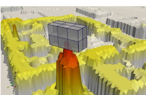
Figure 3.A three-dimensional rendering of the urban topography near Hotel Torni(a)and a close-up featuring the target box (T) for particle capturing(b).
Figure 4. Example discretization of target volume VTinto nx× ny×nzsubvolumes. A coarse illustration withnx=2,ny=3, and nz=2 is shown.
The evaluation procedure (6) closely resembles that of Ran-nik et al. (2003), with the exception that here it is assumed that each particle is represented only once in each subset si,j,k.
The individual sectional footprints are typically evaluated from subsets that contain an insufficient number of parti-cle data entries needed to obtain a converged footprint dis-tribution. (Hellsten et al., 2015) showed that, in an urban-like environment, ∼106 particle hits are required to attain an adequately converged footprint distribution while∼105 particle entries is sufficient to reveal the characteristic shape of the near-field distribution. In the piecewise postprocess-ing approach, the sectional footprint contributions may be constructed from an arbitrarily small dataset, but since the methodology substantially benefits from the ability to inspect and compare individualfi,j,kdistributions, it is desirable to work with subsetssi,j,kcontaining more than 105entries. To facilitate the postprocessing procedure, eachfi,j,kshould be individually stored as a stand-alone two-dimensional scalar
field (i.e., raster map) that can be projected onto the three-dimensional topography model of the LES domain to permit descriptive visualizations in the urban setting. The value of the denominator Di,j,k=Ni,j,k1xf1yf featured in Eq. (6)
has to be stored together with the footprint distribution be-cause the assembly of the final footprint is carried out by computing
f =
P
i,j,k∈KDi,j,kfi,j,k P
i,j,k∈KDi,j,k
, (9)
where K is the set of all i, j, k combinations which have been selected via spatial sensitivity analysis (covered in Sect. 2.3.2).
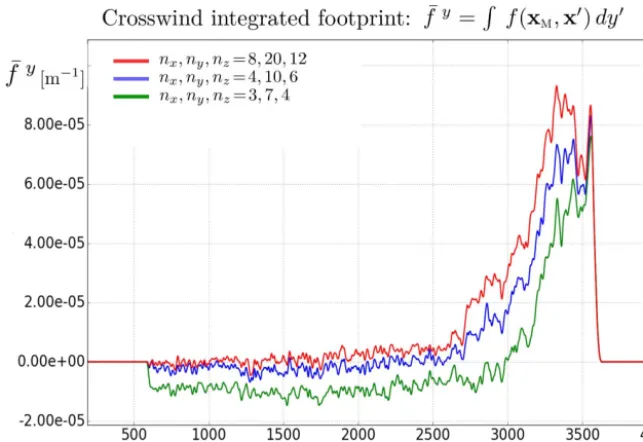
were now directly obtained from their corresponding LES grid cells. Figure 5 illustrates the effect of target volume dis-cretization by comparing crosswind integrated footprintsf¯y at different levels of refinement. The comparison reveals how the negative bias in the far field and the reduction in near-field magnitude immediately emerge with coarser discretizations. It should also be noted that a targeted refinement in thez di-rection, while using coarser horizontal resolution in effort to generate thin subvolumes that approximate planes, does not remedy the situation because the mean flow gradients around the sensor site are significant in all directions. Such finite planes or one-cell-high grid layers are conventionally used as targets when Lagrangian-particle-based methods are utilized to evaluate footprints under heterogeneous conditions with undisturbed sensor sites (e.g., Steinfeld et al., 2008; Hellsten et al., 2015; Glazunov et al., 2016).
Unfortunately, at the required level of target volume dis-cretization, the excessive number of individual fi,j,k con-tributions causes the postprocessing to become highly te-dious. Since the proposed LES–LS methodology is founded on the premise that the size of the original target box around the sensor site can be chosen arbitrarily, the postprocess-ing effort must entail a procedure that enables the exclusion of those fi,j,k contributions that are deemed unfit for the final assembly. However, this selection operation becomes overly laborsome to manage when the number of subvol-umes becomes large (viz. values exceeding 102) and partic-ularly when the individual sectional footprints inadequately converge and thereby become uninformative when examined independently. For instance, in this case study, the required level of discretization gives rise to fi,j,k contributions that are generated from ca. 104 particle entries, which is a de-cidedly insufficient amount even for generating informative approximations for the near-field distributions. For these rea-sons, it is deemed unacceptable that the evaluation of urban footprints solely relies on the established piecewise postpro-cessing method. In response, this paper introduces an aug-mented coordinate rotation technique, labeledfar-field cor-rection, which incorporates well into the proposed piecewise postprocessing strategy and brings significant savings in the associated data manipulation efforts. This alternative tech-nique allows much coarser target volume discretization to be employed in the assembly of the final footprint without un-acceptably compromising the result.
The method has a prerequisite that the deficiently obtained footprint (for instance, obtained via insufficient target box discretization) must exhibit a properly leveled off far field, because the approach fundamentally relies on the following simple assertion: if the footprint distribution plateaus in the far field, this asymptote can be amended to become the zero reference level, which deviates from the “correct” asymptote by a negligibly small offset. Accepting this assertion and the associated approximation paves the way for a corrective co-ordinate rotation scheme which can be laid out by first clas-sifying the data contributing to the far-field footprint via
sub-setsri,j,k⊂si,j,k which are defined as the sets of particle entries whoseXo fall into the outermost portion of the do-main
ri,j,k=
si,j,k
0≤
Xol−Xmino < β 100
xM−Xmino
.
Here Xomin= min l∈{1,...,Nrp}
(Xlo)is the farthest upstream coor-dinate where particles are seeded (thus, farthest away from
xM) andβ specifies the remotest percentage of the footprint across which the mean value off¯yno longer changes, that is,D∂∂xf¯yE≈0 when averaging over the length of the far field. (Theβvalue is case-specific, but a typical range is expected to fall between 10 and 20.) With the help of the far-field datasets ri,j,k, the fluctuating vertical velocity component, used in Eq. (6) and previously defined by Eq. (7), can now be evaluated as
W0Tl=WTl− h ¯wi∗
i,j,k
, (10)
where
h ¯wi∗
i,j,k=ci,j,kh ¯wii,j,k (11)
defines the far-field-corrected mean vertical velocity, which is obtained by scaling the initially obtained value by a coef-ficientci,j,kto satisfy the criterion that the particle entries in eachri,j,kdo not contribute to the correspondingfi,j,k. This becomes a simple one-dimensional optimization problem in which the objective is to minimizeJ=
R
βfi,j,kdx
, where
β represents the far-field domain, by the means of control-lingci,j,k. Thus, this technique bears resemblance to a planar fit method (Wilczak et al., 2001). Because the control vari-able here is a single scalar, a rudimentary implementation of an iterative gradient decent search algorithm suffices (see, for instance, Nocedal and Wright, 2006).
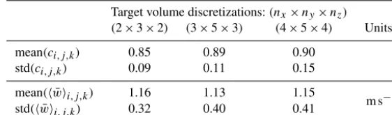
Table 2 displays selected diagnostic data obtained from an application of this far-field correction technique to the Hotel Torni footprint case study. The data indicate that, when the mean vertical velocity values are initially obtained from the LES solution, theci,j,kscaling coefficients concentrate near the mean value of 0.9. The range of individual values natu-rally depends on the magnitude of the starting valueh ¯wii,j,k
in Eq. (11) which, in turn, depends on the chosen discretiza-tion of the target volume. But it is important to emphasize that, although the far-field correction method is guaranteed to yield a physically justifiable asymptotic behavior for the footprint, the combined effect of the correction method and the target volume discretization on the final footprint result cannot be inferred from Table 2.
Figure 5.Crosswind integrated distributions of piecewise postprocessed footprints obtained with different levels of target volume discretiza-tions usingh ¯wii,j,kfrom LES solution. Anomalous contributions from subvolumes immediately behind or in contact with the tower structure were omitted from the assembly (refer to Sect. 2.3.2).
gives rise to an error that is distributed throughout the foot-print domain. Therefore, the validity of the far-field correc-tion approach hinges upon the magnitude of this distributed error and its sensitivity to the target box discretization. The sensitivity can be established by carrying out the selective assembly of the footprint result for different levels of target box discretizations.
2.3.2 Selective assembly of the final footprint
Since its conception it has been clear that the piecewise post-processing approach must be endowed with the capacity to incorporate a sensitivity analysis phase into the final assem-bly of the footprint result. One of the driving motivators for developing the piecewise approach arose from the need to re-duce the computational cost of collecting a large number of particle hits by an arbitrarily sized target volume aroundxM. However, the reduction can only be achieved by the piece-wise postprocessing approach if the sectional footprint re-sults are allowed to be inspected and combined in a par-tially converged state. This is an important stipulation with-out which the proposed postprocessing strategy fails to offer considerable computational savings.
Thus, the process of selectively assembling the final foot-print result begins by first defining an inadequately con-verged initial footprint, which represents the desired preform atxM. This reference footprint, labeledfREF, should be con-structed from at least 106particle entries to facilitate a suffi-ciently informative evaluation of sensitivities. The selection process proceeds by iteratively introducing partial contribu-tionsf(l)that are independent fromfREFand evaluating the
sensitivity of the footprint distribution with respect to the se-lection of target box indices inK(see Eq. 9). The objective is to obtain a sufficiently converged footprint while minimiz-ing the discrepancy between the constituentfi,j,k included in the final result. Thus, the selection process is quantita-tively guided by the evaluation of “deltas” betweenfREFand f(l), constructed from a partial setK(l) of target box indices (i.e.,1f(l)=fREF−f(l)) and utilizing a norm over a subdo-main?⊂encompassing only the near field (a fraction of the total LES footprint domain nearest toxM) as a measure for the associated discrepancy. In this connection, it has been found most effective to define the extent of?such that the integral over the near-field domain constitutes approximately half of the total integral of the footprint:R
?fdx≈
1 2 R
fdx. The near-field norm is computed as
||1f(l)||2,
?=
Z
?
1f
(l)(x f)
2
dxf
1/2
, (12)
utilizing identically normalized footprints for this evalua-tion. In this study the footprints are normalized to yield
R
fdx=1. The exclusion of the outer portion of the foot-print domain allows the relevant deviations in the near field to be reflected in||1f(l)||2,
? while avoiding the contam-ination due to poorly defined “deltas” in the weakly con-verged outer region. In this study, the nearest 30 % of the total length of the LES footprint domain is used to repre-sent the near field as this yields for the normalized reference footprintR
?f
Table 2.Diagnostic data from the application of far-field correction in the coordinate rotation. The farthest 15 % of the source area in the LES domain is considered (i.e.,β=15).
Target volume discretizations:(nx×ny×nz) (2×3×2) (3×5×3) (4×5×4) Units
mean(ci,j,k) 0.85 0.89 0.90
std(ci,j,k) 0.09 0.11 0.15
mean(h ¯wii,j,k) 1.16 1.13 1.15
m s−1 std(h ¯wii,j,k) 0.32 0.40 0.41
herein for the case study utilizing target volume discretiza-tionnx×ny×nz=3×5×3. The relevant intermediate results and||1f(l)||2,
?values are depicted in Fig. 6.
The process begins by setting at the 0th iteration K(0)= {IM,JM,KM} ⊂K, where the indices correspond to the subvol-ume containingxM. The obtained footprintf(0)=fIM,JM,KM
is composed of ca. 4×10⁵ particle entries, which does not meet the desired level of convergence to act asfREF. Thus, through a qualitative inspection, the original set is augmented K(1)=K(0)+ {IM,JM±1,KM}to yieldf(1), which is chosen as the reference footprint.
The iterative process continues such that new candidate contributionsf(l)are introduced incrementally in a radially outward progressing manner. This process is demonstrated in Fig. 6 where intermediate entriesf(2)-f(6)introduce differ-ently combined additions in y, x andzdirections. For the sake of brevity, the example contributions combine a rel-atively large number of fi,j,k entries. The decision to in-clude a candidate contribution in the final assembly is done according to a criteria||1f(l)||2,
?≤ ||1f||max, where the maximum allowable discrepancy ||1f||max must be deter-mined according to the case-specific requirements. In this case study, the threshold was set to include f(3) such that
||1f||max= ||1f(3)||2,
?. Naturally this threshold level can be varied to generate alternative footprint assemblies (with different levels of convergence), which allow, in the context of the considered footprint applications, the impact and un-certainty associated with these choices to be transparently monitored.
The obtained final result, which combines the earlier ac-cepted additions, features 20/45 of all subvolume contri-butions. The obtained footprint also exhibits adequate con-vergence in the far field, having been constructed from ca. 8×10⁶ particle entries. Subsequently, the lowest vertical (k=1) plane and the farthest (i=3) plane were completely excluded from Kin the final assembly. This outcome indi-cates that the contributions with the largest deviations arise fromVi,j,kthat are either in contact with the tower structure or in its wake region. Therefore, this suggests that it is not ad-vantageous to set upVTsuch that the building structure cuts into the volume.
As long as the individual subsets contain a sufficient num-ber of particle data entries (>105), as is required by the
far-field correction approach, it is beneficial to discretize the tar-get volume as finely as possible (by increasingnx,ny, and nz) as it enables a more flexible and fine-tuned assembly and permits a more accurate coordinate rotation treatment. Depending on the total number of particles gathered dur-ing the simulation and the size of the target box, the max-imum number of admissible subvolumes is expected to be
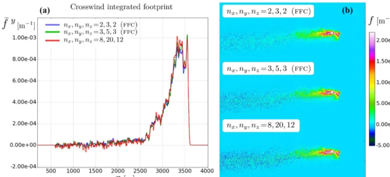
∼102. At this scale, when the postprocessing techniques are implemented with appropriate automations, the labor cost is not significantly affected by the total number of subvol-umes. However, when the standard coordinate rotation is ap-plied and the target volume discretization is carried out in accordance with the LES grid resolution, the total number of subvolumes readily exceeds 103(as in this example study nx×ny×nz=1920) the selective assembly phase becomes prohibitively laborsome. But, given sufficient computational capacity, the far-field correction approach can be exploited to perform the selective assembly process to provide a descrip-tion for an effective target volumeVT,eff =Pi,j,k∈KVi,j,k, which can subsequently be reassembled from the finely re-solvedVi,j,kcontributions. Such a result is depicted in Fig. 7 together with two footprints that are obtained through an identically guided selection process utilizing far-field correc-tion (FFC) with different combinations ofnx,ny, andnz. The comparison reveals that the differences between the three re-sults are remarkably insignificant, indicating, first, that a sig-nificant part of the error contributions, introduced by the far-field correction method, have a compensating effect and, sec-ond, that the obtained footprint is not highly sensitive to the sensor placement despite the variable flow conditions around the sensor. This demonstrates the utility and robustness of the selective piecewise postprocessing approach. From here on the presented results correspond to the nx=3, ny=5, nz=3 target volume discretization level.
2.3.3 Outline of the procedure
Figure 6. Illustration of the selective assembly of the final footprint fornx×ny×nz=3×5×3=45. Values of ||1f(l)||2,? indicating discrepancy betweenfREFandf(l)are shown where applicable. Acceptable candidates are marked byXand the rejected by×. Note the use of short-hand notation, e.g., 1:3=1,2,3.
1. Split the original datasetSintonx×ny×nznumber of subsets labeledsi,j,kaccording to a Cartesian division of the target volumeVT.
2. Evaluate an approximate footprint in a piecewise man-ner by applying Eq. (6) for each subsetsi,j,kand assem-ble the result according to Eq. (9) by selecting alli, j, k values. (Here it is possible to use inaccurate data for the evaluation ofh ¯wii,j,kas the objective is only to identify the far field).
3. Inspect the approximate footprint result to identify the extent of the far field (by specifyingβ) where the foot-print reaches an asymptotic level to a good approxi-mation, and specifyβ for the purpose of constructing ri,j,k.
4. Evaluate the sectional footprintsfi,j,kfrom correspond-ingsi,j,ksubsets by applying Eq. (6) withh ¯wi∗i,j,k eval-uated through far-field correction approach as follows:
a. select initial guess forcoi,j,kandh ¯wio
i,j,k, and utiliz-ing the data fromri,j,kcompute the initial sectional
footprintfi,j,k=fi,j,k(coi,j,k)and the correspond-ing far-field integralJo=
R
βfi,j,k(c o i,j,k)dx
;
b. perturb the coefficient ci,j,k=coi,j,k+dc (ini-tially with a guessed perturbation dc) and, us-ing h ¯wi∗
i,j,k=ci,j,kh ¯wioi,j,k and the data from ri,j,k, compute fi,j,k=fi,j,k(ci,j,k) and J=
R
βfi,j,k(ci,j,k)dx
;
c. exit the loop ifJ < ε, whereεspecifies the toler-ance;
d. compute derivative dJdc =(J−Jo)
dc and specify a new perturbation from dc= −γdJdc, where γ >0 is a scaling parameter which, in this context, has been a experimentally set to ensure that the minimization problems converge sufficiently;
e. setJo=J,coi,j,k=ci,j,kand return to step 4b. 5. Select the appropriate setKofi, j, kcombinations
Figure 7.Comparison of identically normalized footprint distributions(b)and their crosswind integrations(a)obtained either by applying (1) the far-field correction (FFC) method and selective assembly or (2) the standard coordinate rotation while utilizing the uniform 1 m resolution of the LES grid in the target volume discretization. The subvolume contributions included in thenx, ny, nz=8,20,12 result were selected to correspond with the effective target volumeVT,eff=P
i,j,k∈KVi,j,kdetermined via the selective assembly fornx, ny, nz=3,5,3.
It is noteworthy that in step 2 for the approximate foot-print evaluation and in step 4a for the initialization of the optimization loop, the values for the mean vertical veloci-ties h ¯wii,j,k do not have to be accurate. Therefore, the use of vertical velocity data from LES can be omitted altogether, which simplifies the case setup and data handling consider-ably. The approximate values can be obtained more simply, for instance, by evaluating the mean of incident vertical ve-locity value from particle data in eachsi,j,k.
3 Result assessment
The proposed methodology, founded on high-resolution LES–LS analysis and a piecewise postprocessing approach, has been shown to be a reliable, robust, and accessible, al-though computationally expensive, approach to generating topography-sensitive footprints in real urban applications. Since the underlying motivation for this development ef-fort sprung from the need to evaluate the potential error that may arise when analytical, closed-form footprint mod-els are applied to urban flux measurements, this work also proposes a technique to approximate the magnitude of this error in the absence of field validation studies. This approach hinges on the assumption that, in a real urban application, a topography-sensitive footprint obtained through a highly re-solved LES–LS analysis features a higher level of accuracy and a lower level of uncertainty than any available closed-form footprint model.
The proposed assessment technique compares the ob-tained LES–LS footprint result to an analytical model, which belongs to the group of closed-form models that would otherwise be employed in similar studies, by applying the
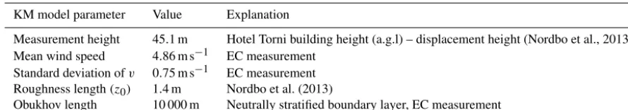
footprint distributions to the land cover classification (LC) dataset in Fig. 1 that is presented at the same resolution as the topography height. In the following demonstration the closed-form footprint model by Korman and Meixner (2001) (KM), which is widely utilized in the EC community (e.g., Christen et al., 2011; Kotthaus and Grimmond, 2012; Nordbo et al., 2013), is used as an example analytical model. This choice is subjective and implies no preference over other available footprint models (e.g., Kljun et al., 2015; Horst, 2001). The KM model parameters and their specific val-ues are declared in Table 3. The mean wind speed and the standard deviation of the crosswind component are extracted from Hotel Torni’s anemometer measurements gathered on 9 September 2012 during the same 30 min time frame that was used to specify the meteorological conditions for the LES simulation (see Sect. 2.2.2).
Table 3.Parameters used in the Korman and Meixner footprint model.
KM model parameter Value Explanation
Measurement height 45.1 m Hotel Torni building height (a.g.l) – displacement height (Nordbo et al., 2013) Mean wind speed 4.86 m s−1 EC measurement
Standard deviation ofv 0.75 m s−1 EC measurement Roughness length(z0) 1.4 m Nordbo et al. (2013)
Obukhov length 10 000 m Neutrally stratified boundary layer, EC measurement
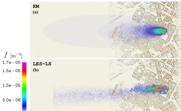
This exhibits the difficulty in choosing one representative pa-rameter value for an analytical model applied to a real urban setting. The most evident deviations occur in the near field, where thefLESexhibits strong local variations between build-ing tops and street canyons. Moreover, examinbuild-ing the cross-wind integrated footprints in Fig. 9 reveals howf¯LESy reacts abruptly to changes in the example urban landscape, leveling off to a shallow descending slope much earlier than the grad-ually declining curve off¯KMy . Thus, the presented comparison in the context of this case study succeeds in laying bare the nontrivial nature of urban footprints and highlights the im-portance of utilizing a high-resolution LES–LS approach to examine complex urban EC measurement sites.
3.1 Virtual assessment technique
The comparative technique proposed for assessing the po-tential error, that may arise if urban measurements are inter-preted with closed-form footprint models, exploits the land cover dataset under the assumption that theLCdistribution conveys the inherent urban heterogeneity sufficiently. Under this premise, theLCdistribution can be adopted as a model distribution of sourcesQsuch that eacheth land cover type is assigned a constant mean source strength hQei =const. Thus, under this simplification the description of a measure-mentηin Eq. (1) can be decomposed as follows:
η(xM)= NLC
X
e=0
ηe(xM)= NLC
X
e=0 Z
e
f (xM,x 0
)hQei dx0, (13)
where the constituents ofηare given by ηe(xM)=
Z
e
f (xM,x 0
)hQei dx0= hQei
Z
e f (xM,x
0 )dx0
= hQeiAe. (14) Here,Aeis the footprint-weighted surface area of theeth land cover type and
e=
Z
LCe
|LCe|
dx0 (15)
defines the corresponding subdomain that leads to =
NLC
X
e=0
e. (16)
Now it is convenient to define two measures that facilitate a meaningful comparison between different footprints: the fractional contribution to the measurement from each con-stituent
re= ηe
P
eηe
, (17)
which require that hQei are assigned for each land cover type, and the source-area fraction
ae= Ae
P
eAe
(18) that provide an easy estimate of the footprint’s coverage inde-pendent of source strength information (or assuming identi-calhQeifor alle). For proper assessment, these two fractions should be inspected in tandem.
The comparison is carried out by extracting the area cor-responding to the LES domain from theLCdataset, shown in Fig. 10, which has been modified to include the relevant streets in the vicinity of the footprint for the purpose of in-cluding the effect of traffic emissions into the demonstration. The obtained fLES and fKM footprints are then projected
onto this raster map to compute the required integrals and fractions.
A pie-chart of source-area fractionsae from Eq. (18) for the Hotel Torni’s flux footprint is demonstrated in Fig. 11, which provides an informative overview on the differences in source-area coverages. The far-field-corrected (nx, ny, nz= 3,5,3) and the highly resolved (nx, ny, nz=8,20,12) piece-wise assembled LES–LS footprints agree within 0.2 %. In this particular example, the analytical KM model gathers a significantly larger contribution from the far-field, which is reflected in the significantly higher coverage of water sur-face area. However, assigning each land cover type its cor-responding – potentially fictional – mean source strength
hQei and evaluating the fractional contributions re from Eq. (17) provides means to carry out simplified virtual exper-iments concerning particular EC measurements. To demon-strate with an example, consider CO2flux measurements in a
hypothetical situation where 95 % of the CO2emissions
Figure 8.Comparison of identically normalized LES–LS(b)and KM(a)footprint distributions merged with the urban topography model of Helsinki. The location of the EC sensor (Hotel Torni) building is indicated with a white circle.
Figure 9.Comparison of normalized, crosswind integrated LES– LS and KM footprints. A light blue dashed line indicates the start of urban topography and the gray dashed line marks the location of the EC sensor.
vegetation is considered to act as a uniformly distributed sink over the land, which does not influence the ratio of source contributions in the measurement. Utilizing an undefined ref-erence source strengthhQrefi, the sources are expressed as
hQei =λehQrefi, where the weights satisfyPeλe=1. Thus, in this example λ0=0.05 for buildings and λ6=0.95 for
roads. For this contrived situation the fractional contributions obtained with the LES–LS footprint becomer0=17.8 % and
r6=82.2 %, whereas applying the Korman–Meixner
foot-print yields r0=16.6 % and r6=83.4 %. In this example,
while the two footprints have distinctly different source-area
fractions for buildings and roads, their ratios are close since (A6/A0)LES=1.1(A6/A0)KM, as seen in Fig. 11, which is
the reason for obtaining such comparable measurement de-compositions.
Repeating the introduced assessment technique for multi-ple representative meteorological conditions paves the way for a numerical approach that allows the obtained urban flux measurements to be interpreted either differently or with im-proved confidence. Naturally, having access to real source strength distributions opens up the ability to utilize LES– LS footprints (or positively assessed analytical footprints) to carry out detailed emission inventories (e.g., Christen et al., 2011).
4 Summary and conclusions
The utility of the eddy-covariance method in measuring the exchanges of mass, heat, and momentum between the urban landscape and the overlying atmosphere largely depends on the ability to determine the effective source area, or footprint, of the measurement. In situations where the heterogeneity of the surface becomes relevant, like for urban landscapes, and the structures surrounding the measurement site can no longer be considered as a homogeneous layer of roughness elements, the use of analytical footprint models becomes highly suspect. In order to diminish the resulting uncertain-ties and to obtain the ability to assess the applicability of ana-lytical models, the ability to evaluate complex footprints with high resolution becomes essential.
mea-Figure 10.Raster map of land cover types,LC, within the LES domain. The original surface type classification data in Fig. 1 has been augmented by adding streets (LC=6) to the relevant footprint area.
Figure 11.Comparison of source-area fractionsaeresulting from applyingfLESandfKMto the raster map of land cover types in Fig. 10.
surement sites. This methodology is based on high-resolution LES–LS analysis where the simulation domain features a de-tailed description of the urban topography and accounts for the entire vertical extent of the atmospheric boundary layer. The online-coupled LS model within the LES solver is em-ployed to simulate a constant release of inert gas emissions from the potential upwind source area of the considered EC sensor. The necessary data for the footprint generation are obtained from the LES–LS analysis by setting up a finite target volume around the sensor location and, over a suffi-ciently long simulation period, gathering a record of parti-cles that hit this target. To generate an estimate for the flux footprint, this dataset is subjected to a postprocessing pro-cedure that involves a coordinate rotation step, which elimi-nates the effect of the mean flow on the flux evaluation. But, if the considered EC sensor is mounted on a building (in-stead of a conventional tower-like structure) in the vicinity of which strong mean flow gradients occur, standard post-processing techniques fail to produce physically meaningful
be reduced significantly. In the piecewise postprocessing ap-proach, the final, completely converged, footprint is eventu-ally selectively assembled from the obtained set of interme-diates.
The methodology is demonstrated in a real urban appli-cation where the objective is to compute a highly resolved topography-sensitive footprint for the Hotel Torni EC flux measurement sensor mounted on the roof of a tall build-ing situated in the downtown area of Helsinki, Finland. The EC sensor’s measurement height is 60 m above the ground level and 36 m above the surrounding mean building height (24 m). The meteorological conditions for the LES simula-tion were adopted from measurements on 9 September 2012 when southwesterly winds and a neutrally stratified boundary layer of 300 m height were recorded. A detailed topography map of Helsinki at 2 m resolution from Nordbo et al. (2015) was utilized to construct the topography model for the LES– LS domain. The resolution of the computational mesh was set at 1 m throughout the domain to ensure that the relevant turbulent structures, even at the level of street canyons, were captured. An arbitrarily sized target box for sampling the La-grangian particle hits was set up around the sensor location, which collected ca. 19×106particle hits during 3 h of simula-tion time. The obtained dataset was subjected to the proposed piecewise postprocessing method, demonstrating the func-tionality of the approach under various user-selected spec-ifications. The obtained footprint stood in stark contrast to gradual ellipse-shaped analytical footprints: the distribution exhibited strong adherence to the building block arrange-ment in the near field, where the weight distribution changed abruptly between roof tops and street canyons. In compari-son to the Korman and Meixner (2001) model, the LES–LS footprint also exhibited stronger contribution from the near field, but more rapidly diminishing contribution from the far field.
This paper also introduces an accessible technique to em-ploy the obtained high-resolution topography-sensitive ur-ban footprint in estimating the potential error that may arise when an analytical footprint model is used to interpret ur-ban EC measurements. The underlying stipulation for this method is that it does not require knowledge of real source strength distributions. Thus, it is proposed that a detailed land cover type classification (LC) dataset is utilized as a model source strength distribution map for the urban surroundings assuming that it reflects the heterogeneity of the urban con-ditions sufficiently. Projecting a footprint distribution result onto such aLC map enables the evaluation fractional con-tributions, which indicate how each land cover type is repre-sented in the measurement. This procedure provides a com-parative technique to assess the effective deviations between different footprints. The demonstrated comparison between the LES–LS and analytical KM footprints in the EC measure-ment setup in Helsinki revealed substantial differences in the fractional contributions when all land cover types are con-sidered equally relevant. The technique can also be applied
by considering only selected land cover types and assign-ing each of them a variable source strength. This approach is demonstrated through a simple example, which mimics a hy-pothetical CO2flux measurement, where the effective source
area is limited to only roads and buildings.
The context of this paper is limited to laying out the new methodology for generating urban footprints and exploiting them in the assessment of analytical models. It is evident that changes in the meteorological and anthropogenic conditions will influence the results and a proper assessment of the ap-plicability of analytical models at a given EC measurement site will require that these conditions are varied, necessitating numerous footprint evaluations. This paper lays the numeri-cal groundwork for such future investigations.
Code availability. PALM is open-source software released under GNU General Public License (v3) and freely available upon reg-istration at https://palm.muk.uni-hannover.de/trac. This study fea-tures version 4.0 and revision 1929. The source code for handling the target box particle data acquisition in PALM is available by request from the corresponding author. The Python scripts used for the topography raster map manipulations and footprint post-processing and analysis are part of a larger library named P4UL, which is primarily developed and maintained by Mikko Auvinen. The code repository for version 1.0-beta is accessible via http: //doi.org/10.5281/zenodo.804851. Python is an open-source pro-gramming language, which is freely available at www.python.org and www.numpy.org. The visualizations are performed with Par-aView, an open-source, multi-platform data analysis and visualiza-tion applicavisualiza-tion, which is freely available at www.paraview.org.
Competing interests. The authors declare that they have no conflict of interest.
Acknowledgements. This study was supported by Academy of Finland (grant no. 284701, 1281255, 277664, and 281255). The computing resources were provided by CSC – IT Center for Science Ltd., Finland (grand challenge project gc2618). The authors would like to sincerely acknowledge Curtis Wood for the meteorological data acquisition and Tiina Markkanen, Siegfried Raasch, Andrey Glazynov, and Juha Lento for the help and advice they provided. The authors also wish to express their gratitude to the peer reviewers whose comments and feedback helped to improve the paper.
References
Anderson, W.: Amplitude modulation of streamwise veloc-ity fluctuations in the roughness sublayer: Evidence from large-eddy simulations, J. Fluid Mech., 789, 567–588, https://doi.org/10.1017/jfm.2015.744, 2016.
Aubinet, M., Vesala, T., and Papale, D. (Eds.): Eddy covariance. A Practical Guide to Measurement and Data Analysis, Springer, 2012.
Christen, A., Coops, N., Crawford, B., Kellett, R., Liss, K., Ol-chovski, I., Tooke, T., van der Laan, M., and Voogt, J.: Valida-tion of modeled carbon-dioxide emissions from an urban neigh-borhood with direct eddy-covariance measurements, Atmos. En-viron., 45, 6057–6069, 2011.
Deardorff, J.: Stratoculumus-capped mixed layers derived from a three-dimensional model, Bound-Lay. Meteorol., 18, 495–527, 1980.
Giometto, M., Christen, A., Meneveau, C., Fang, J., Krafczyk, M., and Parlange, M.: Spatial Characteristics of Rough-ness Sublayer Mean Flow and Turbulence Over a Real-istic Urban Surface, Bound.-Lay. Meteorol., 160, 425–452, https://doi.org/10.1007/s10546-016-0157-6, 2016.
Glazunov, A., Rannik, Ü., Stepanenko, V., Lykosov, V., Auvinen, M., Vesala, T., and Mammarella, I.: Large-eddy simulation and stochastic modeling of Lagrangian particles for footprint deter-mination in the stable boundary layer, Geosci. Model Dev., 9, 2925–2949, https://doi.org/10.5194/gmd-9-2925-2016, 2016. Hellsten, A., Luukkonen, S., Steinfeld, G., Kanani, F., Markkanen,
T., Järvi, L., Vesala, T., and Raasch, S.: Footprint evaluation for flux and concentration measurements for an urban-like canopy with coupled Lagrangian stochastic and large-eddy simulation models, Bound-Lay. Meteorol., 157, 191–217, 2015.
Horst, T.: Comment on Footprint Analysis: A Closed Analytical So-lution Based on Height-Dependent Profiles of Wind Speed and Eddy Viscosity, Bound.-Lay. Meteorol., 101, 435–447, 2001. Järvi, L., Hannuniemi, H., Hussein, T., Junninen, H., Aalto, P. P.,
Hillamo, R., Mäkelä, T., Keronen, P., Siivola, E., Vesala, T., and and Kulmala, M.: The urban measurement station SMEAR III: Continuous monitoring of air pollution and surface-atmosphere interactions in Helsinki, Finland, Boreal Environ. Res., 14 (Suppl. A), 86–109, 2009.
Kataoka, H. and Mizuno, M.: Numerical flow computation around aeroelastic 3-D square cylinder using inflow turbulence, Wind and Structures, An International Journal, 5, 379–392, 2002. Kljun, N., Calanca, P., Rotach, M. W., and Schmid, H. P.:
A simple two-dimensional parameterisation for Flux Foot-print Prediction (FFP), Geosci. Model Dev., 8, 3695–3713, https://doi.org/10.5194/gmd-8-3695-2015, 2015.
Korman, R. and Meixner, F.: An analytical footprint model for non-neutral stratification, Bound-Lay. Meteorol., 99, 207–224, 2001. Kotthaus, S. and Grimmond, C.: Identification of Micro-scale An-thropogenic CO2, heat and moisture sources – Processing eddy covariance fluxes for a dense urban environment, Atmos. Envi-ron., 57, 301–316, 2012.
Kurbanmuradov, O., Rannik, Ü., Sabelfeld, K., and Vesala, T.: Di-rect and Adjoint Monte Carlo Algorithms for the Footprint Prob-lem, Monte Carlo Methods and Applications, 5, 85–112, 1999. Kurppa, M., Nordbo, A., Haapanala, S., and Järvi, L.: Effect of
seasonal variability and land use on particle number and CO2
exchange in Helsinki, Finland, Urban Climate, 13, 94–109, https://doi.org/10.1016/j.uclim.2015.07.006, 2015.
Letzel, M., Helmke, C., Ng, E., An, X., Lai, A., and Raasch, S.: LES case study on pedestrian level ventilation in two neighbourhoods in Hong Kong, Meteorol. Z., 21, 575–589, 2012.
Lund, T., Wu, X., and Squires, K.: Generation of Tur-bulent Inflow Data for Spatially-Developing Boundary Layer Simulations, J. Comput. Phys., 140, 233–258, https://doi.org/10.1006/jcph.1998.5882, 1998.
Maronga, B., Gryschka, M., Heinze, R., Hoffmann, F., Kanani-Sühring, F., Keck, M., Ketelsen, K., Letzel, M. O., Kanani-Sühring, M., and Raasch, S.: The Parallelized Large-Eddy Simulation Model (PALM) version 4.0 for atmospheric and oceanic flows: model formulation, recent developments, and future perspectives, Geosci. Model Dev., 8, 2515–2551, https://doi.org/10.5194/gmd-8-2515-2015, 2015.
Moeng, C. and Wyngaard, J.: Spectral analysis of large-eddy sim-ulations of the convective boundary layer, J. Atmos. Sci., 45, 3573–3587, 1988.
Nocedal, J. and Wright, S.: Numerical Optimization, Springer Se-ries in Operations Research, Springer, 2nd Ed., 2006.
Nordbo, A., Järvi, L., Haapanala, S., Moilanen, J., and Vesala, T.: Intra-city variation in urban morphology and turbulence structure in Helsinki, Finland, Bound-Lay. Meteorol., 146, 469–496, 2013. Nordbo, A., Karsisto, P., Matikainen, L., Wood, C., and Järvi, L.: Urban surface cover determined with airborne lidar at 2 m resolu-tion – implicaresolu-tions for surface energy balance modelling, Urban Climate, 13, 52–72, 2015.
Pasquill, F.: Some aspects of boundary layer de-scription, Q. J. Roy. Meteorol. Soc., 98, 469–494, https://doi.org/10.1002/qj.49709841702, 1972.
Pasquill, F. and Smith, F.: Atmospheric Diffusion, Wiley, New York, 3rd Edn., 1983.
Raasch, S. and Schröter, M.: PALM – A large-eddy simulation model performing on massively parallel computers, Meteorol. Z., 10, 363–372, 2001.
Rannik, Ü., Aubinet, M., Kurbanmuradov, O., Sabelfeld, K., Markkanen, T., and Vesala, T.: Footprint analysis for measure-ments over a heterogeneous forest, Bound.-Lay. Meteorol., 97, 137–166, 2000.
Rannik, Ü., Markkanen, T., Raittila, J., Hari, P., and Vesala, T.: Tur-bulence statistics inside and over forest: Influence on footprint prediction, Bound.-Lay. Meteorol., 109, 163–189, 2003. Saiki, E., Moeng, C., and Sullivan, P.: Large-eddy simulation of the
stably stratified planetary boundary layer, Bound-Lay. Meteorol., 95, 1–30, 2000.
Schmid, H.: Footprint modelling for vegetation atmosphere ex-change studies: a review and perspective, Agr. Forest Meteorol., 113, 159–183, 2002.
Sogachev, A., Menzhulin, G. V., Heimann, M., and Lloyd, J.: A simple three-dimensional canopy–planetary boundary layer sim-ulation model for scalar concentrations and fluxes, Tellus B, 54, 784–819, 2002.
Sogachev, A., Panferov, O., Gravenhorst, G., and Vesala, T.: Numer-ical analysis of flux footprints for different landscapes, Theor. Appl. Climatol., 80, 169–185, 2005.
into large-eddy simulation, Bound-Lay. Meteorol., 129, 225– 248, 2008.
Vesala, T., Järvi, L., Launiainen, S., Sogachev, A., Rannik, Ü., Mammarella, I., Siivola, E., Keronen, P., Rinne, J., Riikonen, A., and Nikinmaa, E.: Surface–atmosphere interactions over com-plex urban terrain in Helsinki, Finland, Tellus B, 60, 188–199, 2008.
Weil, J., Sullivan, P., and Moeng, C.: The use of large-eddy simu-lations in Lagrangian particle dispersion models, J. Atmos. Sci., 61, 2877–2887, 2004.
Wilczak, J. M., Oncley, S., and Stage, S.: Sonic anemometer tilt cor-rection algorithms, Bound.-Lay. Meteorol., 99, 127–150, 2001. Wood, C. R., Järvi, L., Kouznetsov, R. D., Nordbo, A., Joffre,