© Author(s) 2009. This work is distributed under the Creative Commons Attribution 3.0 License.
Model Development
Evaluation of the new UKCA climate-composition model –
Part 1: The stratosphere
O. Morgenstern1,*, P. Braesicke1, F. M. O’Connor2, A. C. Bushell3, C. E. Johnson2, S. M. Osprey4, and J. A. Pyle1
1NCAS-Climate-Chemistry, Chemistry Department, Cambridge University, UK 2Met Office Hadley Centre, Exeter, UK
3Met Office, Exeter, UK
4Sub-Department of Atmospheric, Oceanic and Planetary Physics, University of Oxford, UK *now at: National Institute of Water and Atmospheric Research, Lauder, New Zealand
Received: 17 November 2008 – Published in Geosci. Model Dev. Discuss.: 12 December 2008 Revised: 26 February 2009 – Accepted: 13 March 2009 – Published: 20 March 2009
Abstract. The UK Chemistry and Aerosols (UKCA) model is a new aerosol-chemistry model coupled to the Met Office Unified Model capable of simulating composition and cli-mate from the troposphere to the mesosphere. Here we in-troduce the model and assess its performance with a particu-lar focus on the stratosphere. A 20-year perpetual year-2000 simulation forms the basis of our analysis. We assess basic and derived dynamical and chemical model fields and com-pare to ERA-40 reanalyses and satellite climatologies. Polar temperatures and the lifetime of the southern polar vortex are well captured, indicating that the model is suitable for assessing the ozone hole. Ozone and long-lived tracers com-pare favourably to observations. Chemical-dynamical cou-pling, as evidenced by the anticorrelation between winter-spring northern polar ozone columns and the strength of the polar jet, is also well captured. Remaining problems relate to a warm bias at the tropical tropopause, slow ascent in the tropical pipe with implications for the lifetimes of long-lived species, and a general overestimation of ozone columns in middle and high latitudes.
1 Introduction
Coupled chemistry-climate models (CCMs) are needed to study the multiple links between ozone, greenhouse gases (GHGs), including ozone precursors and ozone-depleting substances (ODSs), and the dynamical components of the climate system. Such models are used to study, e.g., the re-sponse of the ozone layer to climate change and conversely
Correspondence to: O. Morgenstern ([email protected])
the active role of ozone in a changing climate (WMO, 2007; IPCC, 2007). Presently there are only a few CCMs available that cover both tropospheric and stratospheric ozone chem-istry (e.g., J¨ockel et al., 2006; Garcia et al., 2007). How-ever, the links between the two regions are increasingly rec-ognized. For example, it is clear that future changes in strato-spheric ozone will significantly impact tropostrato-spheric compo-sition (Zeng and Pyle, 2003) and surface climate (Morgen-stern et al., 2008). Such coupled models will become in-creasingly widespread. Ozone recovery will likely be as-sociated with decreasing actinic fluxes in the lower strato-sphere, leading to increasing atmospheric lifetimes, and pos-sibly increased abundances, of some long-lived greenhouse gases (GHGs). The Antarctic ozone hole has been associ-ated with substantial climate change in middle to high south-ern latitudes (Thompson and Solomon, 2002); this develop-ment is likely to reverse as the ozone recovers. However, the picture is complicated by simultaneous accumulation of GHGs in the atmosphere, leading to stratospheric cooling, in-creased abundance of polar stratospheric clouds (PSCs) and enhanced chlorine activation, delaying ozone recovery dur-ing polar sprdur-ing. There is also a suggestion, recently chal-lenged, that climate change may lead to a faster overturning of the stratosphere (Waugh, 2009, and references therein). In addition, volcanic eruptions can substantially perturb ozone chemistry and the climate system. Furthering our under-standing of all of these processes usually requires coupled climate-chemistry modelling.
(http://www.ukca.ac.uk), which will form an integral part of the Met Office Unified Model (MetUM). When com-pleted, this model will link aerosol and gas phase chemistry in a troposphere-stratosphere environment. The new model will be used in upcoming World Meteorological Organiza-tion (WMO) ozone and Intergovernmental Panel on Climate Change (IPCC) assessments and will form part of the new QUEST Earth System model (http://quest.bris.ac.uk). The main focus of the present paper is to document the set-up of a stratospheric-chemistry version of UKCA and as-sess its chemical and dynamical performance versus avail-able observations and climatologies. The results presented in this paper derive from an integration of the UKCA model performed as part of our contribution to the Stratospheric Processes And their Role in Climate (SPARC) Chemistry-Climate Model Validation (CCMVal) activity (http://www. atmosp.physics.utoronto.ca/SPARC/index.html; http://www. pa.op.dlr.de/CCMVal/). In the subsequent sections we present a model description, assessments of climate, chem-istry, and chemical-dynamical coupling, and a synthesis of the model performance. The performance of UKCA with re-spect to tropospheric chemistry and aerosols will be the sub-ject of parts 2 and 3 of this publication.
2 Model description
The whole-atmosphere and stratospheric versions of UKCA, called here Strat-UKCA, are based on a middle-atmosphere version of the MetOffice Unified Model (MetUM) with 60 levels in the vertical, a top lid at 84 km, and a horizontal resolution of 3.75◦×2.5◦. Morgenstern et al. (2008) use the
model to study the impact on climate of ozone loss avoided by the Montreal Protocol; the version used here is almost identical to theirs. The dynamical core of the model is de-scribed by Davies et al. (2005). Due to the model’s non-hydrostatic formulation the vertical coordinate system in the model is hybrid-height, unlike most climate models. Ad-vection in the model is semi-Lagrangian (Priestley, 1993). Gravity wave drag comprises an orographic (Webster et al., 2003) and a parameterized spectral component (Scaife et al., 2002); the latter addresses momentum transport from the tro-posphere to the middle atmosphere. Radiation follows Ed-wards and Slingo (1996) with 9 bands in the long- and 6 in the shortwave part of the spectrum. In the version con-sidered here the model is run in an atmosphere-only mode forced with prescribed sea surface temperatures (SSTs) and sea ice. Here, perpetual year-2000 SSTs and sea ice from the HadISST climatology (Rayner et al., 2003) are used.
For Strat-UKCA we have added to the model a com-prehensive description of stratospheric chemistry, includ-ing chlorine and bromine chemistry and heterogeneous pro-cesses on polar stratospheric clouds (PSCs) and liquid sul-phate aerosols (based on Chipperfield and Pyle, 1998). Note that a simplified tropospheric chemistry is also included. The
Table 1. Species predicted by Strat-UKCA. Highlighted in bold
are species that feed into the radiation, underlined are species that experience dry deposition, and italicised are species that are wet-deposited. Other radiatively active species comprise O2, CO2, and
H2O.
O1D, O3P, O3,
H, OH, HO2, H2O2,
N, NO, NO2, NO3, N2O5, HONO2, HO2NO2, N2O,
CH4, CH3O2, CH3OOH, HCHO, CO,
Cl, ClO, OClO, Cl2O2, HCl, HOCl, ClONO2, CFCl3, CF2Cl2,
Br, BrO, BrCl, HBr, HOBr, BrONO2, CH3Br
chemistry is embedded in a flexible way using the ASAD framework (Carver et al., 1997), built around a symbolic non-families sparse-matrix Newton-Raphson solver (derived from Wild and Prather, 2000). Table 1 summarizes the species predicted by the chemistry part of Strat-UKCA. O2,
N2, H2, and CO2 are not predicted by the chemistry and
are assumed uniform. Chemical water production or loss is deliberately ignored in the chemistry and instead a pa-rameterization for stratospheric water vapour production is used based on Untch et al. (1998) which assumes a uniform distribution of equivalent water H2O+2CH4=6.03 ppmv. We
also set water vapour equal to 3.5 ppmv in the tropical lower stratosphere (between 30◦S and 30◦N and between 18 and 23 km). This procedure is followed because this model ver-sion has a warm bias above the tropical tropopause (see be-low). Chemical reactions and their respective references are summarized in Tables 2–5. Bimolecular and termolecular reaction rates are amalgamated from Atkinson et al. (2000) and Sander et al. (2003), as indicated in Tables 2 and 3. Pho-tolysis rates are defined following the procedure outlined be-low (Table 4): Where available, photolysis in the troposphere (below 300 hPa) follows tabulated rates calculated off-line in the Cambridge 2-D model (updated from Harwood and Pyle, 1975), as also used by the Cambridge TOMCAT (Law et al., 1998) and UM UCAM (Zeng and Pyle, 2003) models. In the stratosphere (above 200 hPa), and in the troposphere for species not included in TOMCAT, a second set of off-line precalculated rates updated from Lary and Pyle (1991), as used by Chipperfield (1999), is used. The stratospheric photolysis rates respond to changes in the overhead ozone column. In the intermediate region (between 200 and 300 hPa) a linear transition is made between the two rates. On-line photolysis rates using the FAST-J2 scheme (Bian and Prather, 2002) are available in the model but are not used here due to the omission of scattering at short wavelengths which would be important for polar ozone chemistry; this has been corrected in the more recent FAST-JX scheme (Neu et al., 2007). We plan to incorporate FAST-JX in future ver-sions of UKCA. Some photolysis reactions with branching
(ClONO2, BrONO2, HO2NO2)have been updated following
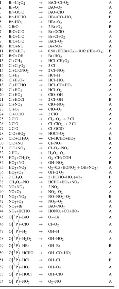
Table 2. Bimolecular reactions in Strat-UKCA. A=Atkinson et
al. (2003). B=Sander et al. (2002).
1 Br+Cl2O2 → BrCl+Cl+O2 A
2 Br+O3 → BrO+O2 A
3 Br+OClO → BrO+ClO A
4 Br+HCHO → HBr+CO+HO2 B
5 Br+HO2 → HBr+O2 A
6 2 BrO → 2 Br+O2 B
7 BrO+ClO → Br+OClO A
8 BrO+ClO → Br+Cl+O2 A
9 BrO+ClO → BrCl+O2 A
10 BrO+NO → Br+NO2 A
11 BrO+HO2 → 0.98(HOBr+O2)+ 0.02(HBr+O3) B
12 BrO+OH → Br+HO2 A
13 Cl+CH4 → HCl+CH3O2 A
14 Cl+Cl2O2 → 3 Cl A
15 Cl+ClONO2 → 2 Cl+NO3 A
16 Cl+H2 → HCl+H A
17 Cl+H2O2 → HCl+HO2 A
18 Cl+HCHO → HCl+CO+HO2 A
19 Cl+HO2 → HCl+O2 A
20 Cl+HO2 → ClO+OH A
21 Cl+HOCl → 2 Cl+OH B
22 Cl+NO3 → ClO+NO2 A
23 Cl+O3 → ClO+O2 A
24 Cl+OClO → 2 ClO A
25 2 ClO → Cl2+O2→2 Cl A
26 2 ClO → Cl+ClO2→2 Cl A
27 2 ClO → Cl+OClO A
28 ClO+HO2 → HOCl+O2 A
29 ClO+CH3O2 → Cl+HCHO+HO2 B
30 ClO+NO → Cl+NO2 A
31 ClO+NO3 → Cl+O2+NO2 A
32 2 HO2 → H2O2+O2 A
33 HO2+CH3O2 → O2+CH3OOH A
34 HO2+NO → OH+NO2 B
35 HO2+NO3 → O2+0.5(HONO2+OH+NO2) A
36 HO2+O3 → OH+2 O2 A
37 2 CH3O2 → 2(HCHO+HO2)+O2 B
38 CH3O2+NO → HCHO+HO2+NO2 A
39 NO+NO3 → 2 NO2 A
40 NO+O3 → NO2+O2 A
41 NO2+NO3 → NO+NO2+O2 B
42 NO2+O3 → NO3+O2 A
43 NO3+Br → BrO+NO2 A
44 NO3+HCHO → HONO2+CO+HO2 A
45 O3P+BrO → O2+Br A
46 O3P+ClO → Cl+O2 A
47 O3P+H2 → OH+H A
48 O3P+H2O2 → OH+HO2 A
49 O3P+HBr → OH+Br B
50 O
3P+HCHO → OH+CO+HO
2 A
51 O
3P+HCl → OH+Cl B
52 O
3P+HO
2 → OH+O2 A
53 O
3P+HOCl → OH+ClO A
54 O
3P+NO
2 → O2+NO A
Table 2. Continued.
55 O3P+NO3 → O2+NO2 A
56 O3P+O3 → 2 O2 A
57 O3P+OClO → O2+ClO A
58 O
3P+OH → O
2+H A
59 O
1D+HBr → 0.2hHBr+O3Pi+0.8 (OH+Br) A
60 O
1D+CH
4 → 0.9(OH +CH3O2)+0.1(HCHO+H2) A
61 O
1D+CO
2 → O
3P+CO
2 A
62 O
1D+H
2 → OH+H A
63 O
1D+H
2O → OH+OH A
64 O
1D+HCl → 0.09hO3P+HCli A
+0.24 (H+ClO)+ 0.67 (OH+Cl)
65 O1D+N2 → O
3P
+N2 A
66 O1D+N2O → 0.42(N2+O2)+1.16 NO B
67 O1D+O2 → O
3P
+O2 A
68 O1D+O3 → 1.5 O2+O
3P
A
69 OClO+NO → NO2+ClO A
70 OH+CH4 → H2O+CH3O2 A
71 OH+CO → H+CO2 A
72 OH+ClO → HO2+Cl B
73 OH+ClO → HCl+O2 B
75 OH+H2O2 → H2O+HO2 A
74 OH+H2 → H2O+H A
76 OH+HBr → H2O+Br A
77 OH+HCHO → H2O+CO+HO2 A
78 OH+HCl → H2O+Cl A
79 OH+HO2 → H2O+O2 A
80 OH+HOCl → ClO+H2O B
81 OH+HONO2 → H2O+NO3 A
82 OH+CH3OOH → H2O+CH3O2 A
83 OH+NO3 → HO2+NO2 B
84 OH+O3 → HO2+O2 A
85 OH+OClO → HOCl+O2 A
86 2 OH → H2O+O
3P B
87 O
3P+ClONO
2 → ClO+NO3 B
88 OH+ClONO2 → HOCl+NO3 B
89 OH+HO2NO2 → H2O+NO2O2 B
90 Cl+CH3OOH → HCl+CH3O2 B
91 CFCl3+O
1D → 2 Cl+ClO B
92 CF2Cl2+O
1D → Cl+ClO B
93 CH3Br+OH → Br+OH B
94 CH3Br+O
1D
→ Br+O3P B
95 CH3Br+Cl → Br+Cl B
96 N+O2 → NO+O
3P
B
97 N+NO → N2+O
3P
B
98 N+NO2 → N2O+O
3P B
99 H+O3 → OH+O2 B
100 H+HO2 → 1.38 OH+0.29(H2+O2) B
+0.02hO3P+H2O
i
Table 3. Termolecular reactions in Strat-UKCA. A=Atkinson et al.
(2000). B=Sander et al. (2003).
1 BrO+NO2+M → BrONO2+M A 2, 3 Cl2O2+ M ↔ 2 ClO+M A
4 ClO+NO2+M → ClONO2+M A 5 2 HO2+M → H2O2+O2+M A
6, 7 HO2+NO2+M ↔ HO2NO2+M A
8, 9 N2O5+ M ↔ NO2+NO3+M A
10 2 NO+ M → 2 NO2+M A
11 O3P+ NO +M → NO2+M B
12 O
3P+ NO
2+M → NO3+M A
13 O3P+ O2+M → O3+M A
14 O1D+ N2+M → N2O+M B
15 OH+ NO2+M → HONO2+M A
16 2 OH+M → H2O2+M A
17 H+ O2+M → HO2+M B
Chipperfield (1999). The abundance of nitric acid trihydrate (NAT) and mixed NAT/ice polar stratospheric clouds is cal-culated following Chipperfield (1999) assuming thermody-namic equilibrium with gas-phase HNO3and water vapour.
Also the treatment of reactions on liquid sulfate aerosol fol-lows Chipperfield (1999).
Species with wet and dry deposition are indicated in Ta-ble 1; dry deposition applies to the bottom level of the model and deposition velocities are calculated in the same way as in Law et al. (1998) and Zeng and Pyle (2003). Wet depo-sition again follows Law et al. (1998). Lightning emissions of NO follow Price and Rind (1992) with total nitrogen pro-duced by lightning scaled to 5 Tg(N)/year. Halogen source gases are treated in a simplified way, with only the major source species CFCl3, CF2Cl2, and CH3Br represented and
lumped with other long-lived contributors, preserving num-bers of chlorine and bromine atoms, respectively (Table 6; Chipperfield, 1999). Wet and dry deposition of inorganic halogen species are not represented; instead, these species are removed instantaneously at the surface. GHGs and ODSs are prescribed at the lowest model level; the boundary layer parameterization (Lock et al., 2000) propagates these signals throughout the boundary layer.
Nitric acid trihydrate (NAT) PSCs are assumed to be in equilibrium with gas phase HNO3. Sedimentation of PSCs
is included in the model. Dehydration is handled as part of the MetUM hydrological cycle. Denitrification is prescribed in the same way as in Chipperfield (1999) with two differ-ent sedimdiffer-entation velocities for pure NAT (0.46 mm/s) and mixed ice/NAT (17 mm/s).
The model is formulated in such a way that halogen load-ings remain invariant under chemistry and are unaffected by dry and wet deposition. For a simulation with invari-ant lower boundary conditions and appropriate
initializa-Table 4. Photolysis reactions in Strat-UKCA. For details on the
method see text. A=Chipperfield (1999), B=Law et al. (1998), C=Sander et al. (2003). “A, C” means that the cross section follows A and the branching ratio follows C. “A, B” means that the pho-tolysis rate follows A above 200 hPa, and B below 300 hPa, with a linear transition inbetween. “A, B, C” means the same as “A, B” but with the branching ratio following C.
1 BrCl+hν → Br+Cl A
2 BrO+hν → Br+O3P A
3 BrONO2+hν → 0.29(Br+NO3)+0.71(BrO+NO2) A,C
4 O2+hν → 2 O3P A, B, C
5 O2+hν → O
3P+O1D A, C
6 O3+hν → O2+O3P A, B
7 O3+hν → O2+O
1D A, B
8 OClO+hν → O3P+ClO A
9 NO+hν → N+O3P A
10 NO2+hν → NO+O3P A, B
11 NO3+hν → NO+O2 A, B
12 NO3+hν → NO2+O3P A, B
13 HOBr+hν → OH+Br A
14 HONO2+hν → NO2+OH A, B
15 HO2NO2+hν → 0.67(NO2+HO2)+ A, B, C 0.33(NO3+OH)
16 N2O+hν → N2+O1D A
17 N2O5+hν → NO2+NO3 A, B
18 H2O+hν → OH+H A
19 H2O2+hν → 2 OH A, B
20 ClONO2+hν → Cl+NO3 A, C
21 ClONO2+hν → ClO+NO2 A, C
22 HCl+hν → H+Cl A
23 HOCl+hν → OH+Cl A
24 Cl2O2+hν → 2 Cl+O2 A
25 HCHO+hν → H+CO+HO2 A, B
26 HCHO+hν → H2+CO A, B
27 CH3OOH+hν → HCHO+HO2+OH A, B
28 CFCl3+hν → 3 Cl A
29 CF2Cl2+hν → 2 Cl A
30 CH3Br+hν → Br A
31 CH4+hν → CH3O2+H A
32 CO2+hν → CO+O
3P A
Table 5. Heterogeneous reactions in Strat-UKCA. Rates are from
Chipperfield (1999).
1 ClONO2+H2O → HOCl+HONO2 2 ClONO2+HCl → Cl2O2+HONO2
3 HOCl+HCl → Cl2O2+H2O 4 N2O5+H2O → HONO2+HONO2
5 N2O5+HCl → OClO+NO2+HONO2
Table 6. Lumping of halogen source gases.
CFCl3 CFCl3, CCl4, CH3Cl, CH3CCl3, CH3CFCl2, CH3CF2Cl, CF2ClBr
CF2Cl2 CF2Cl2, CF2ClCFCl2,(CF2Cl)2, C2F5Cl, CHF2Cl
CH3Br CH3Br, CF2ClBr, CF3Br,(CF2Br)2, CF2Br2
Table 7. (a) Surface boundary conditions needed for chemistry:
Volume mixing ratios (VMRs) for CH4, N2O, and halogen source
gases. Clyand Brydenote total chlorine and total bromine,
respec-tively. (b) Surface VMRs for the CFCs and CO2 (needed for
radiation). 3-dimensional distributions for the CFCs are obtained by rescaling the lumped fields.
(a)
CH4 N2O CFCl3 CF2Cl2 CH3Br Cly Bry
1.77E-6 316E-9 632E-12 723E-12 17.5E-12 3.34E-9 17.5E-12
(b)
CFCl3 CF2Cl2 CO2
262E-12 539E-12 369E-6
circumvent this problem we introduce total chlorine and to-tal bromine as advected tracers. These tracers then do not have sharp gradients in the stratosphere. For transport they replace the most abundant inorganic forms of chlorine and bromine, HCl and BrO. The model then well preserves total chlorine and total bromine. A total odd nitrogen tracer, re-placing NO2, is also introduced, which also includes the
frac-tion of N2O that goes on to form odd nitrogen (6.9%). Due
to the special treatment of water vapour (see above) hydro-gen is not explicitly conserved in the model; this feature can be included once the tropical tropopause warm bias has been reduced. This aspect of the model is expected to improve in a planned future version with a new advection scheme which will be linear in tracers.
3 The simulation
In the following we present the results of a 30-year time-slice simulation of Strat-UKCA, following the definition of the REF-B0 experiment of CCMVal. In this experiment, forcings represent perpetual year-2000 conditions. Boundary conditions and global abundances, respectively, of GHGs and ODSs are listed in Table 7. CO2 is assumed uniform
with an abundance of 369 ppmv. Aircraft emissions of NO and surface emissions of NO, CO, and HCHO are the av-erage over the years 1998, 1999, and 2000 emissions taken from the RETRO database (Schultz et al., 2007). The to-tal halogen loadings are around 3.4 ppbv for chlorine and
17.5 pptv for bromine. We prescribe a perpetual year 2000 aerosol surface area density updated from SPARC (2006), as described by Eyring et al. (2008); this affects reactions 3 and 4 in Table 5. Aerosols are at background levels, i.e., vol-canic eruptions are not considered in the simulation. Note that bromine species considered in REF-B0 deliberately ex-clude very short-lived bromine source gases which would contribute 3–8 pptv to stratospheric bromine (WMO, 2007). Species with feedback into the radiation are highlighted in Table 1. For radiation, the CFCs (CFCl3and CF2Cl2) are
scaled to their surface abundance, following the A1b scenario (Houghton et al., 2001), without lumping. The first 10 years of the simulation, during which the model settles down, are ignored; results pertain to the last 20 years of the run.
4 Model performance
4.1 Dynamical aspects
4.1.1 Mean temperature, winds and humidity
Figure 1 shows the 20-year temperature climatology pro-duced by the model, which is compared to a climatology derived from the ERA-40 reanalysis data set (Uppala et al., 2005), using the years 1979 to 2001. The model satisfacto-rily reproduces tropospheric zonal-mean temperatures, and in the stratosphere the southern polar vortex is well repre-sented. The northern polar vortex above 100 hPa is also well captured. Elsewhere, some biases remain, e.g., in the upper stratosphere (above 10 hPa), and around 100 hPa year-round in the tropics. The warm bias around 100 hPa means that without additional constraints too much water would enter the stratosphere. As an aside, versions of the MetUM with prescribed ozone do not exhibit any appreciable bias in this region, suggesting that this is an ozone-sensitive result. How-ever, the realistic temperatures above Antarctica mean that there can be substantial chlorine activation in the southern polar vortex, allowing us to assess the model’s performance in reproducing Antarctic ozone.
Fig. 1. Multiannual, seasonal- and zonal-mean temperatures in K
in Strat-UKCA (colours) and in the ERA-40 dataset using the years 1979–2001 (contours).
Figure 3 indicates that water vapour is generally well rep-resented. ERA-40 has got a slightly more pronounced de-hydration during Antarctic winter; also dede-hydration does not extend below 100 hPa. The upper-stratospheric abundance of water vapour is very similar to the ERA-40 climatology. Also the position of the transition to tropospheric humidity (around 6 ppmv) is quite similar between the two data sets. In the troposphere, away from the tropical UTLS region there is good agreement. In the upper tropical troposphere, around 200 hPa, ERA-40 predicts somewhat more water vapour than Strat-UKCA. Note that the seasonal cycle of water vapour around 70 hPa in the tropics evident in ERA-40 is suppressed in the model by artificially prescribing water vapour there (Sect. 2).
4.1.2 The Quasi-Biennial Oscillation (QBO)
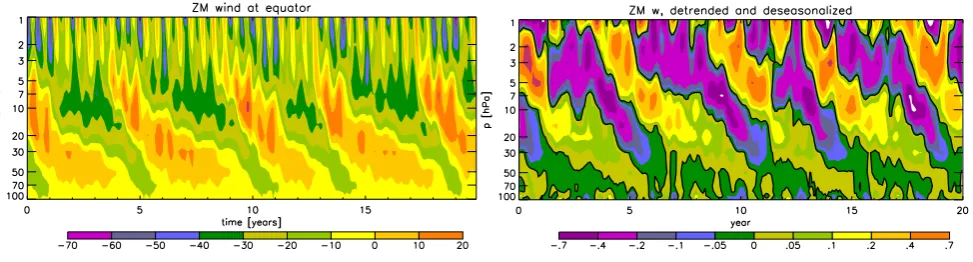
An analysis of equatorial winds (Fig. 4, left) reveals that there is a well-formed oscillation in the lower stratosphere, with amplitudes of 10 to 20 m/s for the westerly phase and −30 to −40 m/s for the easterly phase. Both compare well with observations (Naujokat, 1986). Its period length of around 4.5 years however is significantly too long, compared with an observed average periodicity of the Quasi-Biennial Oscillation (QBO) of around 27 months. The periodicity is substantially longer than the one found in the equivalent
Fig. 2. Same as Fig. 1 but for zonal wind, in m/s.
Fig. 3. Same as Fig. 1 but for water vapour volume mixing ratio, in
Fig. 4. (left) Monthly- and zonal-mean zonal winduin Strat-UKCA at the Equator, in m/s. (right) Deseasonalized, detrended and smoothed zonal-mean vertical windw∗at the Equator, in mm/s.
version without interactive chemistry, indicating a sensitivity to ozone (Butchart et al., 2003). It can be changed by varying the source strength in the spectral gravity wave deposition; this re-tuning has not been done for this model version. The presence of the oscillation however sets the model apart from the majority of the models compared by Eyring et al. (2006) that do not have an internally generated QBO.
The QBO is known to modulate upwelling in the tropics. Following Fleming et al. (2002), Fig. 4 (right) shows the de-trended, deseasonalized, and smoothed vertical windsw∗at the Equator throughout the integration. A comparison with Fig. 4 (left) shows thatw∗ correlates very well with zonal winds, as in Fleming et al. (2002); also the typical peak-to-peak amplitude (Fig. 4, right) compares well with Fig. 1 of Fleming et al. (2002).
4.1.3 The polar vortices
Figure 5 displays the probability density function (PDF)
P (A)of an areaAocurring with temperatures below 195 K at 50 hPa. It is evaluated for both Strat-UKCA and ERA-40 and separately for both hemispheres, excluding areas equatorwards of±45◦. The PDF is calculated from daily snapshots of temperature at 00:00 UTC. For the Arctic, Fig. 5 suggests that small to medium-size vortices (less than 10×1012m2) are well represented, but the probability for large vortices is underestimated. For the Antarctic, both in Strat-UKCA and ERA-40 there are preferred sizes for the polar vortex. In the ERA-40 data this is around 23×1012m2. Strat-UKCA underestimates this with around 19×1012m2, with consequences for the simulation of the Antarctic ozone hole.
The timing of the onset of Antarctic summer, as indicated by a reversal from westerlies to easterlies at the latitude of the polar jet, has been challenging for models to reproduce correctly (Eyring et al., 2006, see Fig. 6), with many models producing a late onset of summer. The zonal-mean winds turn to easterlies starting aloft and propagating downwards
Fig. 5. The PDF for, at any time of the year, the area with
temper-atures below 195 K at 50 hPa. The PDF is constructed from daily snapshots at 00:00 UTC. Solid: Strat-UKCA. Dotted: ERA-40 for the years 1979–2002. Black: Northern Hemisphere (latitude>45◦). Orange: Southern Hemisphere (latitude<−45◦).
during the course of the months of November to January. The timing of breakup in our model compares favourably with the ERA-40 data set (Fig. 6), with deviations from the ERA-40 mean limited to less than the standard deviation throughout the depth of the domain.
4.1.4 Age of air and the tape recorder signal
Fig. 6. Timing of the transition of the zonal-mean zonal wind from westerlies to easterlies at 60◦S. Left: Black contour: UKCA mean wind. Violet solid: ERA-40 mean wind. Dashed: ERA-40 plus and minus the standard deviation of ERA-40. Ticks mark the beginning of the month. Right: Same for 12 models and 3 analyses (Fig. 2 of Eyring et al., 2006). Reproduced with kind permission by AGU.
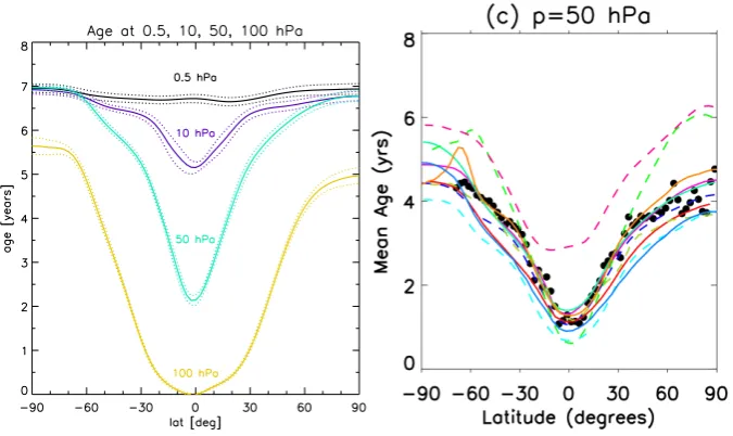
Fig. 7. Left: Annual-zonal mean age of air in Strat-UKCA at 100, 50, 10, and 0.5 hPa, with the mean age at the Equator at 100 hPa defined
as 0. Dotted lines indicate the age plus and minus its standard deviation. Right: Annual-zonal mean age at 50 hPa from ER-2 observations of CO2and from a variety of models (Fig. 10c of Eyring et al., 2006). Reproduced with kind permission by AGU.
age at the Equator at 100 hPa. Figure 7 shows the 20-year mean age, with the interannual standard deviation, at differ-ent pressures, compared to observations and models. As ex-pected, due to the periodic forcings the interannual variabil-ity of annual-mean age, expressed by the standard deviation, is typically just a few months; this also indicates that any trend due to insufficient spin-up must be insignificant. There is about a 2-year difference in age in the tropics between 100 and 50 hPa, which is quite large compared to measurements and most models. The difference between mean equatorial and south-polar age at 50 hPa of around 4.7 years is also larger than suggested by Eyring et al. (2006). It appears
that upward motion in the tropical pipe is too slow, leading to these problems. Consequences for chemistry and radiation, and a possible link to the tropical-tropopause warm bias, are discussed in the subsequent sections.
Fig. 8. Left: Multiannual- and zonal-mean total bromine VMR at the Equator, minus global-mean bromine, times 1015(ppfv), from Strat-UKCA. Right: Multiannual- and zonal-mean water vapour volume mixing ratio at the Equator, minus the mean equatorial water profile, in ppbv, from ERA-40 (1979–2002). Shown are two annual cycles.
(MLS) climatology (Fig. 8 of Eyring et al., 2006) and in the ERA-40 water vapour. There is a considerable difference in the speed of upward propagation between these two data sets, with HALOE/MLS suggesting slower upward propaga-tion than ERA-40. Resolving this discrepancy is beyond the scope of this paper; however, there is a possibility that strato-spheric water vapour in ERA-40 may be insufficiently con-strained by observations and may mainly reflect an ECMWF model property. The HALOE/MLS tape recorder signal sug-gests an age difference between 100 and 10 hPa in the tropics of around 20 months; Strat-UKCA is largely in agreement with this number. Considering the aforementioned problems with age of air, further comparisons with independent data would be beneficial, e.g. the satellite products compared by Chiou et al. (1992).
4.2 Chemical constituents 4.2.1 Ozone
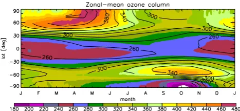
Figure 9 shows the modelled zonal-mean ozone column latitude-time section, with the SBUV/TOMS climatology (Stolarski and Frith, 2006) superimposed. All the major fea-tures in the diagram look similar to the climatology and their timing is captured realistically. In the tropics, both the mag-nitude of the column and its standard deviation (2–5 Dobson Units, DU, not shown) compare very well with observations. In northern high latitudes, Strat-UKCA overestimates the springtime ozone maximum by 60 to 80 DU, but also the minimum in summer is slightly overestimated. In southern midlatitudes, we find again a year-round overestimation of the ozone column by 20 to 60 DU. Antarctic ozone reaches mean values of less than 180 DU in October. Observations suggest a slightly deeper mean ozone hole for present-day conditions, of less than 150 DU. However, the contrast with midlatitudes is quite realistic. The standard deviation maxi-mizes at 50 DU in early spring in the Arctic and late spring in
Fig. 9. Multiannual- and zonal-mean ozone column (Dobson Units). Colours: Strat-UKCA, with daily resolution. Contours: TOMS/SBUV climatology, with monthly resolution.
the Antarctic, respectively, mainly reflecting the differences in the life cycles of the polar vortices. A comparison with Fig. 14 of Eyring et al. (2006) suggests that in the tropics and mid-latitudes Strat-UKCA is within the range spanned by other models; for polar latitudes the comparison is inap-propriate because Eyring et al. (2006) evaluate a transient simulation with significant changes in polar halogen load-ings whereas here we study a time-slice experiment with in-variant, historically high halogen loadings.
Fig. 10. Multiannual-, monthly-, and zonal-mean ozone in ppmv in (top) September and (bottom) February. (left) Colours: Strat-UKCA.
Black contours: HALOE/MLS climatology. White contours: The Fortuin and Langematz (1995) climatology, restricted top>70 hPa. (right) Scatter plot of Strat-UKCA versus HALOE/MLS ozone. Black line: 1:1 line. Black symbols: Pressurep≥10 hPa. Green symbols; p<10 hPa. Orange line: Linear regression fit. The parameters of the regression (slope, axis intercept, in ppmv, and the correlation coefficient) are stated in the titles of the plots (Russell et al., 1993).
Langematz (1995). This feature possibly reflects the slow up-draft found before in the tropical lower stratosphere. There may also be excessive ozone production here due to insuf-ficient UV absorption at higher levels where ozone is un-derestimated. Elsewhere in the free troposphere, in the ex-tratropics the model generally seems to overestimate ozone. The Antarctic ozone hole is present in the data; however, the depth is underestimated with ozone mixing ratios not drop-ping below 1 ppmv below 40 hPa, unlike suggested by the HALOE/MLS climatology. Figure 13 of Eyring et al. (2006) suggests that most CCMs, like ours, overestimate ozone in the lower-stratosphere region.
A detailed evaluation of the tropospheric performance of UKCA is the subject of part 2 (Sect. 1).
4.2.2 Methane and nitrous oxide
For CH4 we perform a comparison versus the
HALOE/Cyrogenic Limb Array Etalon Spectrometer (CLAES) climatology (Fig. 11; Kumer et al., 1993). In general, the two CH4distributions are quite similar, although
with some important differences. In the tropics, modelled CH4 appears to fall off too quickly with height. In the
southern polar vortex, a tongue of very methane-depleted air extends down from the mesosphere and, e.g. between 100 and 1 hPa, depresses the CH4mixing ratio below values
suggested by HALOE/CLAES. For N2O, essentially the
Fig. 11. Multiannual-, monthly-, and zonal-mean (left) CH4 in ppmv and (right) N2O in ppbv, in September. Colours: Strat-UKCA. Contours: CH4: HALOE/CLAES climatology. N2O: CLAES climatology.
Fig. 12. Multiannual-, monthly-, and zonal-mean (left) HNO33 and (right) NOx=NO2+NO in September, in ppbv. Colours: Strat-UKCA.
Contours: HNO3: CLAES climatology. NOx: HALOE climatology (average of sunrise and sunset data).
subsidence of air of mesospheric origin in the Antarctic polar vortex; the steep decline of methane in the tropical pipe is also related to the slow ascent in the tropical pipe. 4.2.3 Odd nitrogen
Odd nitrogen in the stratosphere mostly results from N2O
oxidation, with (in our model) 6.9% of N2O forming NOy,
the rest returning N2. In the lower stratosphere, the
domi-nant form of odd nitrogen is HNO3. Generally, compared
to the CLAES climatology the shape of the distribution of nitric acid is well represented but the model somewhat over-estimates its abundance (Fig. 12). Above 10 hPa, the domi-nant form of odd nitrogen is NOx(=NO+NO2). A reference
HALOE NOxclimatology is constructed by taking the sum
of the four sunrise and sunset NO and NO2climatologies,
di-vided by 2. In comparison with this reference, the model gets the shape of the distribution about right but the magnitude is overestimated, reflecting the too rapid decline of N2O with
altitude.
4.2.4 Hydrogen chloride
Fig. 13. Multiannual-, monthly-, and zonal-mean HCl in ppbv in (left) September and (right) February. Colours: Strat-UKCA. Contours:
HALOE climatology.
Table 8. Global atmospheric lifetimes of long-lived species, in
years. The uncertainty indicates the interannual standard deviation of the annual-mean lifetimes. *excluding the terrestrial sink.
species N2O CFCl3 CF2Cl2 CH4
Strat-UKCA 161±3 88±3 146±3 9.07±0.03
Houghton et al. (2001) 120 45 100 8.9*
period of 1978–1993, during which time the average chlo-rine loading was indeed lower than the loading imposed for Strat-UKCA (Table 7). Also note the evidence for chlorine activation in southern high latitudes, e.g., the isolated min-imum of HCl at 70◦S and 50 hPa. In February there is ev-idence for weaker chlorine activation in the Arctic, with a localized minimum of HCl forming between 50 and 90 hPa in the Arctic, in good agreement with HALOE.
4.2.5 Lifetimes of long-lived species
The lifetime of long-lived species is defined here as the mean abundance of a given species during a model year, di-vided by the total throughput through all loss channels dur-ing this year. Table 8 summarizes the finddur-ings. The CH4
lifetime compares favourably to Houghton et al. (2001) in-dicating that tropospheric OH abundances are broadly cor-rect. For the other long-lived tracers with large tropospheric sinks (CH3Br, H2) important surface sinks are excluded from
the budget, leading to a substantial overestimation of the lifetimes. The errors in N2O and the CFCs reflect a
gen-uine problem of this model version. These species are al-most exclusively photochemically destroyed in the strato-sphere; the very slow updraft in the tropical pipe noted ear-lier (Sect. 4.1.4) implies that these species are not destroyed quickly enough.
4.3 Climate-chemistry coupling
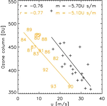
Braesicke and Pyle (2003) find a strong anticorrelation be-tween the northern polar ozone column and the strength of the polar jet, peaking (in their model) at a correlation coeffi-cient of−0.91 in January. Here we assess the performance of Strat-UKCA in this respect, versus available observational data. Note that satellite data do not cover the Arctic in Jan-uary; we focus here on March when the northern polar vortex is still intact and satellite used here achieves a partial cover-age of the polar region. Figure 14 shows the Arctic ozone column in March, as a function of a measure of the strength of the polar jet. The correlation coefficient of−0.76 is almost the same as that derived from NIMBUS-7/TOMS data (Heath and Park, 1978) and ERA-40 reanalyses (Uppala et al., 2005) for the same variables. This suggests that despite the obvious offset of around 50 DU produced by the model the coupling between ozone column and jet strength is well represented in the model. Strat-UKCA actually produces strong anticorre-lations for all winter months. As an aside, Morgenstern et al. (2008) use Strat-UKCA to study a world with 9 ppbv of total chlorine in the atmosphere (2.7 times the amount used here); they find that this relationship has broken down at 9 ppbv of total chlorine.
Fig. 14. Monthly-zonal-mean March zonal wind u at 60◦N and 100 hPa, versus monthly-zonal-mean March ozone column at 77.5◦N. Linear regressions are superimposed. Black symbols: Strat-UKCA. Orange numbers: Observations, marked by the years of the 20th century. Zonal winds are from ERA-40 analyses. Ozone columns are constructed from daily NIMBUS-7 TOMS (Heath and Park, 1978) total ozone maps. Note that at 77.5◦N TOMS measure-ments start on 6 or 7 March, so the mean is from 6 or 7 March to 31 March. rstands for the correlation coefficient,mfor the linear regression coefficient.
geographical distrubution of significant positive or negative correlations. A verification of EP flux-ozone column change correlations using observations is complicated by a need for high temporal resolution of meteorological analyses and is thus beyond the scope of this paper.
5 Synthesis of model performance and outlook
The model comparison versus satellite and other climatolog-ical datasets suggests that in many respects the model per-forms quite well. With the exception of tropical tropopause temperatures, in the multiannual mean all basic meteoro-logical fields analyzed here compare favourably with ERA-40. The size of the Antarctic polar vortex is underestimated by around 3×10¹²m2, but the timing of its disappearance in spring compares very well with ERA-40. October mean Antarctic ozone columns drop to 160 to 180 DU, indicating a somewhat weak ozone depletion in the Antarctic. The Arc-tic polar vortex is well captured; only the probability of rare large vortices (greater than 1013m2) is underestimated. The model produces a QBO but with a periodicity of around 4.5 years which is too large compared to observations. Age of air is older than suggested by observations and most other models, with the maximum age difference between the trop-ical tropopause and 0.5 hPa reaching 7 years. This
prop-Fig. 15. Correlation coefficient, derived from Strat-UKCA, of the
mean change of zonal-mean ozone column in a month,1O3/1t, with the vertical component of the EP flux at 100 hPa. The data have been binned in 10◦latitude bands for the analysis.
erty is also reflected in an upward propagation of the tape recorder signal which is slower than in the ERA-40 reanal-yses. It however compares favourably to the UARS/MLS climatology. This aspect requires further investigation. The slow upwelling causes an overestimation of chemical life-times of species with dominant stratospheric sinks (N2O and
the CFCs). The methane lifetime by contrast is well cap-tured, indicating a broadly correct OH abundance in the tro-posphere. It appears from N2O and CH4that subsidence over
the South Pole in winter is too fast, possibly suppressing the signature of ozone loss by removing ozone-depleted air and activated chlorine from the ozone loss region. The model has a tendency to overestimate the abundance of ozone in mid-dle and high latitudes generally, meaning that polar ozone depletion is likely to start off from a high starting point. Strat-UKCA produces a strong anticorrelation between Arc-tic ozone columns and the strength of the polar jet which is very similar to observations. An evaluation of EP fluxes reveals that seasonally at high latitudes there are strong cor-relations between the vertical component of the EP flux and changes in the ozone column. These two quantities also an-ticorrelate at lower latitudes. Qualitatively these findings are similar to literature assessments but there are important dif-ferences in seasonality.
non-orographic part of it (Scaife et al., 2002) can be tuned to adjust the periodicity of the QBO. Temperature at the tropical tropopause may be more sensitive to the orographic compo-nent (Webster et al., 2003). Increasing the upwelling in this region might simultaneously reduce stratospheric age-of-air, remove some ozone from the tropopause region, thus cool this region, and reduce the lifetimes of long-lived gases. Re-tuning the model would need to broadly preserve tempera-tures in the polar vortices.
We conclude that for a contemporary atmosphere the model well reproduces the basic mean meteorological state of the stratosphere almost everywhere, with the exception of the tropical tropopause. The chemical fields analyzed here likewise resemble observations. The chemical-dynamical coupling that characterizes the Arctic polar vortex is well captured. A more comprehensive tropospheric chemistry (similar to Zeng and Pyle, 2003) and an interactive aerosol scheme (Spracklen et al., 2007) will be evaluated in parts 2 and 3 of this publication. Further developments will include nudging (Telford et al., 2008) and interactive photolysis (Neu et al., 2007).
Acknowledgements. This work is supported by the Natural Environment Research Council (NERC) through the NCAS initiative and by the European Commission under the Framework 6 SCOUT-O3 IP. F. M. O’Connor, C. E. Johnson and part of the development of UKCA were supported by the Joint DECC, Defra and MoD Integrated Climate Programme – DECC/Defra (GA01101), MoD (CBC/2B/0417 Annex C5). ECMWF ERA-40 data used in this study have been obtained from the ECMWF data server. We acknowledge the American Geophysical Union for use of copyrighted material.
Edited by: P. Joeckel
References
Andrews, D. G., Holton, J. R., and Leovy, C. B.: Middle Atmo-sphere Dynamics, Academic Press, 489 pp., 1987.
Atkinson, R., Baulch, D. L., Cox, R. A., Hampson, R. F., Kerr, J. A., Rossi, M. J., and Troe, J.: Evaluated kinetic and photochem-ical data for atmospheric chemistry: Supplement VIII, IUPAC Subcommittee on Gas Kinetic Data Evaluation and Atmospheric Chemistry, J. Phys. Chem. Ref. Data, 29, 167–266, 2000. Bian, H. and Prather, M. J.: FAST-J2: Accurate simulation of
strato-spheric photolysis in global chemical models, J. Atmos. Chem., 41, 281–296, 2002.
Braesicke, P. and Pyle, J. A.: Changing ozone and chang-ing circulation in northern mid-laitudes: Possible feedbacks?, Geophys. Res. Lett., 30(2), 1059, doi:10.1029/2002GL015973, 2003.
Butchart, N., Scaife, A. A., Austin, J., Hare, S. H. E., and Knight, J. R.: Quasi-biennial oscillation in ozone in a coupled chemistry-climate model, J. Geophys. Res., 108(D15), 4486, doi:1029/2002JD003004, 2003.
Chiou, E. W., McCormick, M. P., McMaster, L. R., Chu, W. P., Larsen, J. C., Rind, D., and Oltmans, S.: Intercomparison
of stratospheric water vapor observed by satellite experiments: Stratospheric Aerosol and Gas Experiment II versus Limb In-frared Monitor of the Stratosphere and Atmospheric Trace Molecule Spectroscopy, J. Geophys. Res., 98(D3), 4875–4887, 1992.
Chipperfield, M. P. and Pyle, J. A.: Model sensitivity studies of Arctic ozone depletion, Geophys. Res. Lett., 103(D1), 28389– 28403, 1998.
Chipperfield, M. P.: Multiannual simulations with a three-dimensional chemical transport model, J. Geophys. Res., 104(D1), 1781–1805, 1999.
Carver, G. D., Brown, P. D., and Wild, O.: The ASAD atmospheric chemistry integration package and chemical reaction database, Computer Phys. Comm., 105(2–3), 197–215, 1997.
Davies, T., Cullen, M. J., Malcolm, A. J., Mawson, M. H., Stan-iforth, A., White, A. A., and Wood, N.: A new dynami-cal core for the Met Office’s global and regional modelling of the atmosphere, Qt. J. Roy. Meteor. Soc., 131, 1759–1782, doi:10.1256/qj.04.101, 2005.
Edwards, J. M. and Slingo, A.: Studies with a flexible new radia-tion code. I: Choosing a configuraradia-tion for a large-scale model, Q. J. Roy. Meteor. Soc., 122, 689–719, 1996.
Eyring, V., Butchart, N., Waugh, D. W., et al.: Assessment of tem-perature, trace species, and ozone in chemistry-climate model simulations of the recent past, J. Geophys. Res., 111, D22308, doi:10.1029/2006JD007327, 2006.
Eyring, V., Chipperfield, M. P., Giorgetta, M. A., Kinnison, D. E., Manzini, E., Matthes, K., Newman, P. A., Pawson, S., Shep-herd, T. G., and Waugh, D. W.: Overview of the new CCM-Val reference and sensitivity simulations in support of upcoming ozone and climate assessments and the planned SPARC CCM-Val, SPARC Newsletter, 30, 20–26, 2008.
Fleming, E. L., Jackman, C. H., Rosenfield, J. E., and Consi-dine, D. B.: Two-dimensional model simulations of the QBO in ozone and tracers in the tropical stratosphere, J. Geophys. Res., 107(D23), 4665, doi:10.1029/2001JD001146, 2002.
Fortuin, J. P. F. and Langematz, U.: An update on the global ozone climatology and on concurrent ozone and temperature trends, Proceedings SPIE, Atmospheric Sensing and Modeling, 2311, 207–216, 1995.
Garcia, R. R., Marsh, D. R., Kinnison, D. E., Boville, B. A., and Sassi, F.: Simulation of secular trends in the mid-dle atmosphere, 1950–2003, J. Geophys. Res., 112, D09301, doi:10.1029/2006JD007485, 2007.
Hall, T. M., Waugh, D. W., Boering, K. A., and Plumb, R. A.: Evaluation of transport in stratospheric models, J. Geophys. Res., 104, 18815–18840, 1999.
Harwood, R. S. and Pyle, J. A.: 2-dimensional mean circulation model for atmosphere below 80 km, Q. J. Roy. Meteor. Soc., 101(430), 723–747, 1975.
Heath, D. F. and Park, H.: The solar backscatter ultraviolet (SBUV) and total ozone mapping spectrometer (TOMS) experiment, The Nimbus 7 Users’ Guide, edited by: C. R. Madrid, Management and Technical Services Company, Beltsville, MD, The Land-sat/Nimbus Project, NASA/GSFC, p. 175, 1978.
IPCC: Climate Change 2007: The Physical Science Basis, Con-tribution of Working Group I to the Fourth Assessment Report of the Intergovernmental Panel on Climate Change, edited by: Solomon, S., Qin, D., Manning, M., Chen, Z., Marquis, M., Av-eryt, K. B., Tignor, M., and Miller, H. L., Cambridge University Press, Cambridge, United Kingdom and New York, NY, USA, 996 pp., 2007
J¨ockel, P., Tost, H., Pozzer, A., Br¨uhl, C., Buchholz, J., Ganzeveld, L., Hoor, P., Kerkweg, A., Lawrence, M. G., Sander, R., Steil, B., Stiller, G., Tanarhte, M., Taraborrelli, D., van Aardenne, J., and Lelieveld, J.: The atmospheric chemistry general circulation model ECHAM5/MESSy1: consistent simulation of ozone from the surface to the mesosphere, Atmos. Chem. Phys., 6, 5067– 5104, 2006,
http://www.atmos-chem-phys.net/6/5067/2006/.
Kumer, J. B., Mergenthaler, J. L., and Roche, A. E.: CLAES CH4,
N2O and CCl2F2(F12) global data, Geophys. Res. Lett., 20(12),
1239–1242, 1993.
Lary, D. and Pyle, J. A.: Diffuse-radiation, twilight, and photo-chemistry.1., J. Atmos. Chem., 13(4), 393–406, 1991.
Law, K. S., Plantevin, P. H., Shallcross, D. E., Rogers, H. L., Pyle, J. A., Grouhel, C., Thouret, V., and Marenco, A.: Evaluation of modeled O3using Measurement of Ozone by Airbis In-Service
Aircraft (MOZAIC) data, J. Geophys. Res., 103(D19), 25721– 25737, 1998.
Lock, A P.,A. R. Brown, M. R. Bush, G. M. Martin, and R. N. B. Smith: A new boundary layer mixing scheme. Part I: Scheme description and single-column model tests, Mon. Weather Rev., 128, 3187–3199, 2000.
Morgenstern, O., Braesicke, P., Hurwitz, M. M., O’Connor, F. M., Bushell, A. C., Johnson, C. E., and Pyle, J. A.: The World Avoided by the Montreal Protocol, Geophys. Res. Lett., 35, L16811, doi:10.1029/2008GL034590, 2008.
Naujokat, B.: An update of the observed quasi-biennial oscillation of the stratospheric winds over the tropics, J. Atmos. Sci., 43, 1873–1877, 1986.
Neu, J. L., Prather, M. J., and Penner, J. E.: Global atmospheric chemistry: Integrating over fractional cloud cover, J. Geo-phys. Res., 112, D11306, doi:10.1029/2006JD008007, 2007. Price, C. and Rind, D.: A simple lightning parameterization for
cal-culating global lightning distributions, J. Geophys. Res., 97(D9), 9919–9933, 1992.
Priestley, A.: A quasi-conservative version of the semi-Lagrangian advection scheme, Mon. Weather Rev., 121(2), 621–629, 1993. Randel, W. J., Wu, F., and Stolarski, R.: Changes in column ozone
correlated with the stratospheric EP flux, J. Meteorol. Soc. Japan, 80(4B), 849–862,2002.
Rayner, N. A., Parker, D. E., Horton, E. B., Folland, C. K., Alexan-der, L. V., Rowell, D. P., Kent, E. C., and Kaplan, A.: Global analyses of sea surface temperature, sea ice, and night marine air temperature since the late nineteenth century, J. Geophys. Res., 108(D14), 4407, 10.1029/2002JD002670, 2003.
Russell, J. M. III, Gordley, L. L., Park, J. H., Drayson, S. R., Hes-keth, W. D., Cicerone, R. J., Tuck, A. F., Frederick, J. E., Harries, J. E., and Crutzen, P. J.: The Halogen Occultation Experiment, J. Geophys. Res., 98(D6), 10777–10797, 1993.
Sander, S. P., Friedl, R. R., Golden, D. M., et al.: Chemical kinet-ics and photochemical data for use in atmospheric studies, JPL Publications 02-25, 2003.
Scaife, A. A., Butchart, N., Warner, C. D., and Swinbank, R.: Im-pact of a spectral gravity wave parametrization on the strato-sphere in the Met Office Unified Model, J. Atmos. Sci., 59, 1473–1489, 2002.
Schultz, M., Rast, S., van het Bolscher, M., et al.: Emission data sets and methodologies fir estimating emissions, Work package 1, Deilverable D1-6, Reanalysis of tropospheric chemical compo-sition over the past 40 years, A long-term global modeling study of tropospheric chemistry funded under the 5th EU framework programme, http://retro.enes.org/reports/D1-6 final.pdf, 2007. SPARC: SPARC assessment of stratospheric aerosol properties
(ASAP), Tech. Rep. WMO-TD No. 1295, WCRP Series Report No. 124, SPARC Report No. 4, Berrieres le Buisson, Cedex, 2006.
Spracklen, D. V., Pringle, K. J., Carslaw, K. S., Mann, G. W., Mank-telow, P., and Heintzenberg, J.: Evaluation of a global aerosol microphysics model against size-resolved particle statistics in the marine atmosphere, Atmos. Chem. Phys., 7, 2073–2090, 2007, http://www.atmos-chem-phys.net/7/2073/2007/.
Stolarski, R. S. and Frith, S. M.: Search for evidence of trend slow-down in the long-term TOMS/SBUV total ozone data record: the importance of instrument drift uncertainty, Atmos. Chem. Phys., 6, 4057–4065, 2006,
http://www.atmos-chem-phys.net/6/4057/2006/.
Telford, P. J., Braesicke, P., Morgenstern, O., and Pyle, J. A.: Tech-nical Note: Description and assessment of a nudged version of the new dynamics Unified Model, Atmos. Chem. Phys., 8, 1701– 1712, 2008,
http://www.atmos-chem-phys.net/8/1701/2008/.
Thompson, D. W. J., and S. Solomon, Interpretation of recent Southern Hemisphere climate change, Science, 296, 5569, 895– 899, 2002.
Untch, A., Simmons, A., et al.: Increased stratospheric resolution in the ECMWF forecasting system, ECMWF Newsletter, 82, 2–8, 1998.
Uppala, S. M., Kallberg, P. W., Simmons, A. J., et al.: The ERA-40 re-analysis, Q. J. Roy. Meteor. Soc., 131, 2961–3012, doi:10.1256/qj.04.176, 2005.
Waugh, D., Atmospheric dynamics: The age of stratospheric air, Nature Geosci., 2, 14–16, doi:10.1038/ngeo397, 2009.
Webster, S., Brown, A. R., Cameron, D. R., and Jones, C. P.: Im-provements to the representation of orography in the Met Office Unified Model, Q. J. Roy. Meteor. Soc., 129, 1989–2010, 2003. Wild, O. and Prather, M. J.: Excitation of the primary tropospheric
chemical mode in a three-dimensional model, J. Geophys. Res., 105(D20), 24647–24660, 2000.