www.geosci-model-dev.net/10/85/2017/ doi:10.5194/gmd-10-85-2017
© Author(s) 2017. CC Attribution 3.0 License.
Variational assimilation of land surface temperature within the
ORCHIDEE Land Surface Model Version 1.2.6
Hector Simon Benavides Pinjosovsky1,5,6, Sylvie Thiria1,3, Catherine Ottlé5, Julien Brajard1,2, Fouad Badran4, and Pascal Maugis5
1Sorbonne University, UPMC Univ Paris 06 CNRS-IRD-MNHN, LOCEAN Laboratory 4 place Jussieu,75005 Paris, France 2Inria Paris, 75012 Paris, France
3UVSQ, 78035 Versailles, France
4Laboratoire CEDRIC, Conservatoire National des Arts et Métiers, 292, rue Saint Martin, 75003 Paris, France
5Laboratoire des Sciences du Climat et de l’Environnement (LSCE), UMR 8212, CNRS-CEA-UVSQ, Orme des Merisiers,
91191 Gif-sur-Yvette, France
6CLIMMOD Engineering, Orsay, France
Correspondence to:Hector Simon Benavides Pinjosovsky ([email protected]) and Sylvie Thiria ([email protected])
Received: 23 March 2016 – Published in Geosci. Model Dev. Discuss.: 14 April 2016 Revised: 7 November 2016 – Accepted: 16 November 2016 – Published: 6 January 2017
Abstract. The SECHIBA module of the ORCHIDEE land surface model describes the exchanges of water and energy between the surface and the atmosphere. In the present paper, the adjoint semi-generator software called YAO was used as a framework to implement a 4D-VAR assimilation scheme of observations in SECHIBA. The objective was to deliver the adjoint model of SECHIBA (SECHIBA-YAO) obtained with YAO to provide an opportunity for scientists and end users to perform their own assimilation. SECHIBA-YAO allows the control of the 11 most influential internal parameters of the soil water content, by observing the land surface tempera-ture or remote sensing data such as the brightness temper-ature. The paper presents the fundamental principles of the 4D-VAR assimilation, the semi-generator software YAO and a large number of experiments showing the accuracy of the adjoint code in different conditions (sites, PFTs, seasons). In addition, a distributed version is available in the case for which only the land surface temperature is observed.
1 Introduction
Land surface models (LSMs) simulate the interactions be-tween the atmosphere and the land surface, which directly influence the exchange of water, energy and carbon with
the atmosphere. They are important tools for understanding the main interaction and feedback processes simulating the present climate and making predictions of future climate evo-lution (Harrison et al., 2009). Such predictions are subject to considerable uncertainties, which are related to the difficulty in modeling the highly complex physics with a limited set of equations that does not account for all the interacting pro-cesses (Pipunic et al., 2008; Ghent et al., 2011). Understand-ing these uncertainties is important in order to obtain more realistic simulations.
assim-ilation period, for Gaussian errors (not correlated in time) and linear models. This property does not stand if the processes under study are nonlinear. The main advantage of 4D-VAR comes from its integration in time achieved during the assim-ilation of the observations, giving rise to a global trajectory of the model optimized over the assimilation time window.
Variational data assimilation has been widely used in land surface applications. The assimilation of land surface tem-perature (LST) is suitable for an extensive range of environ-mental problems. As mentioned in Ridler et al. (2012), LST is an excellent candidate for model optimization since it is a solution of the coupled energy and water budgets, and per-mits one to constrain parameters related to evapotranspira-tion and indirectly to soil water content.
Castelli et al. (1999) expose a variational data assimila-tion approach, including surface energy balance in the es-timation procedure as a physical constraint (based on ad-joint techniques). The authors worked with satellite data and directly assimilated soil skin temperatures. They concluded that constraining the model with such observations improves model flux estimates, with respect to available measure-ments. Huang et al. (2003) developed a one-dimensional land data assimilation scheme based on an ensemble Kalman fil-ter, used to improve the estimation of the land surface tem-perature profile. They demonstrated that the assimilation of LST into land surface models is a practical and effective way to improve the estimation of land surface state variables and fluxes.
Reichle et al. (2010) performed the assimilation of satellite-derived skin temperature observations using an ensemble-based, offline land data assimilation system. Re-sults suggest that the retrieved fluxes provide modest but sta-tistically significant improvements. However, these authors noted strong biases between LST estimates from in situ ob-servations, land modeling, and satellite retrievals that vary with season and time of the day. They highlighted the im-portance of taking these biases into account; otherwise, large errors in surface flux estimates can result.
Ghent et al. (2011) investigated the impacts of data assim-ilation on terrestrial feedbacks of the climate system. Assim-ilation of LST helped to constrain simulations of soil mois-ture and surface heat fluxes. Ridler et al. (2012) tested the ef-fectiveness of using satellite estimates of radiometric surface temperatures and surface soil moisture to calibrate a soil– vegetation–atmosphere transfer (SVAT) model, based on er-ror minimization of temperature and soil moisture model out-puts. Flux simulations were improved when the model is cal-ibrated against in situ surface temperature and surface soil moisture versus satellite estimates of the same fluxes.
Bateni et al. (2013) employed the full heat diffusion equa-tion to perform a variaequa-tional data assimilaequa-tion. Deviaequa-tion terms of the evaporation fraction and a scale coefficient were added as penalization terms in the cost function. A weak constraint was applied to data assimilation with model un-certainty, accounting in this way for model errors. The cost
function associated with this experiment contains a term that penalizes the deviation from prior values. When assimilating LST into the model, the authors proved that the heat diffusion coefficients are strongly sensitive. As a conclusion, it can be seen that the assimilation of LST can improve the model sim-ulated flows.
In the present study, we focused on the SECHIBA mod-ule (Ducoudré et al., 1993), which is part of the ORCHIDEE land surface model dedicated to the resolution of the surface energy and water budgets. Our objective was to test the abil-ity of 4D-VAR to estimate a set of its inner parameters. A dedicated software (called SECHIBA-YAO) was developed by using the adjoint semi-generator software called YAO de-veloped at LOCEAN-IPSL (Nardi et al., 2009). YAO serves as a framework to design and implement dynamical mod-els, helping to generate the adjoint of the model, which per-mits one to compute the model gradients. SECHIBA-YAO provides an opportunity to control the most influent inter-nal parameters of SECHIBA by assimilating LST (land sur-face temperature) observations. At a given location and for specific soil and climate conditions, twin experiments of as-similation have been executed. These twin experiments con-ducted on actual sites were used to demonstrate the accuracy and usefulness of the code and the potential of 4D-VAR when dealing with LST assimilation.
This paper is structured as follows. In Sect. 2, model and data used to illustrate the capabilities of the SECHIBA-YAO are detailed. In Sect. 3, fundamentals of variational data as-similation are presented. In addition, principles of YAO and of its associated modular graph formalism are shown. The principle of the computation of the adjoint with YAO is pro-vided. The implementation of SECHIBA-YAO and the de-tails of the experiments that prove the efficiency of the 4D-VAR assimilation are also given in Sect. 3. Sensitivity exper-iments and simple twin experexper-iments at two FLUXNET lo-cations are presented in Sect. 4. These experiments illustrate the convenience of YAO to optimize control parameters. Sec-tion 5 consists in a discussion and a conclusion. Finally, the specificities of the distributed software are given in Sect. 6.
2 Models and data
processes related to the carbon cycle, such as carbon dynam-ics, the allocation of photosynthesis respiration and growth maintenance, heterotrophic respiration and phenology, and finally, LPJ (Sitch et al., 2003) models the global dynam-ics of the vegetation, interspecific competition for sunlight as well as fire occurrence. ORCHIDEE has different timescales: 30 min for energy and matter, 1 day for carbon processes and 1 year for species competition processes. The full descrip-tion of ORCHIDEE can be found in Ducoudré et al. (1993), Krinner et al. (2005), d’Orgeval et al. (2006), and Kuppel et al. (2012). In the present study, ORCHIDEE version 1.9 is used in a grid-point mode (at a given location), forced by the corresponding local half-hourly gap-filled meteorologi-cal measurements obtained at the flux towers. In this study, only the SECHIBA module is considered.
In SECHIBA, the land surface is represented as a whole system composed of various fractions of vegetation types called PFTs (plant functional types). A single energy bud-get is performed at each grid point, but the water budbud-get is calculated for each PFT fraction. The resulting energy and water fluxes between atmosphere, ground and the retrieved temperature represent the canopy ensemble and the soil sur-face. The main fluxes modeled are the net radiation (Rn),
soil heat flux (Q), sensible (H) and latent heat (LE) fluxes between the atmosphere and the biosphere, land surface tem-perature (LST) and the soil water reservoir contents. Energy balance is solved once, with a subdivision only for LE in bare soil evaporation, interception and transpiration for each type of vegetation. Water balance is computed for each fraction of vegetation (plant functional type or PFT) present in the grid. The SECHIBA version used in this work models the hydrological budget based on a two-layer soil profile (Chois-nel, 1977). The two soil layers represent, respectively, the surface and the total rooting zone. The soil is considered ho-mogeneous with no sub-grid variability and a total depth of htot=2 m. The soil bottom layer acts like a bucket that is
filled with water from the top layer. The soil is filled from top to bottom with precipitation; when evapotranspiration is higher than precipitation, water is removed from the upper reservoir. Runoff arises when the soil is saturated. SECHIBA inputs are Rlw the incoming infrared radiation;Rsw the
in-coming solar radiation; P the total precipitation (rain and snow); Ta the air temperature; Qa the air humidity; Ps the
atmospheric pressure at the surface andUthe wind speed. In the full version of SECHIBA-YAO, observations of LST or brightness temperature can be used to constrain model in-ner parameter or initial conditions of the model variables. However, the simulated LST is hemispheric and does not ac-count for solar configuration and viewing angle effects. In order to compute a thermal infrared brightness temperature from LST, and neglecting the directional effects, the total en-ergy emitted by the surface (Rad) can be computed using the following expression:
Rad=kemisεLST4+(1−ε kemis)LWdown. (1)
In this equation,εis the surface emissivity,kemisis the
multi-plicative factor for emissivity and LWdownis the longwave
in-cident radiation that is an input forcing of SECHIBA. Svend-sen et al. (1990) proposed a transfer function to link the sur-face emitted radiance towards an observed brightness tperature TB measured in the [8,14] spectral band. The em-pirical formulation is given by the expression
TB=
Rad−7.84
6.7975.1011
0.2
. (2)
In the following, the capabilities of the 4D-VAR are demon-strated in a series of assimilation experiments using the data provided by the FLUXNET network (Baldocchi et al., 2001). FLUXNET is a network coordinating regional and global analysis of observations from micrometeorological tower sites. The flux tower sites use eddy covariance meth-ods (Aubinet et al., 2012) to measure the exchange of carbon dioxide (CO2), water vapor, and energy between terrestrial
ecosystems and the atmosphere. SECHIBA-YAO can be run using other data as long as the same inputs needed to operate SECHIBA are given.
Measurement towers sprang up around the world, grouped into regional networks. The data from all networks are ac-cessible to the scientific community via the FLUXNET web-site (http://www.fluxdata.org). In this work, we selected two sites: Harvard Forest and Skukuza Kruger National Park; both present contrasted climate and land surface properties suitable for testing the tools developed and assessing model parameter sensitivities. Only climate measurements with the same sampling frequency (30 min) from both sites are used to force SECHIBA. Vegetation characteristics are prescribed and only homogeneous grids are considered. Two cases were studied with agricultural C3 (PFT 12) and bare soil (PFT 1). 2.1 Skukuza Kruger National Park
Located in South Africa at 25◦101100S and 31◦2904800E, this FLUXNET site was established in 2000. The tower overlaps two distinct savanna types and collects informa-tion about land–atmosphere interacinforma-tions. The climate is subtropical–Mediterranean. The total mean annual precipi-tation is 650 mm, with an altitude of 150 m, and the mean annual temperature is 22.15◦C.
2.2 Harvard Forest
3 The methodology
3.1 Variational assimilation
Variational assimilation (4D-VAR) (Le Dimet et al., 1986) considers a physical phenomenon described in space and its time evolution. It thus requires the knowledge of a direct dy-namical modelM, which describes the time evolution of the physical phenomenon. M computes geophysical variables, which are compared to observations. By varying some model parameters (control parameters), assimilation seeks to infer geophysical variables that are the closet to observation val-ues (LST in the present case). The control parameters can be, as an example, initial conditions or physical parameters ofMleading to the computation of LST.
The basic idea is to determine the minimum of a cost func-tionJthat measures the misfits between the observations and the model estimations. Due to the complexity of this func-tion, the solution is classically obtained by using gradient methods, which implies the use of the adjoint model ofM. This model is derived from the equations of the direct model M. The adjoint model estimates changes in the control vari-ables in response to a disturbance of the output values calcu-lated byM. It is done by integrating the same model in the backward direction (e.g., time integration is from the future to the past). If observations are available, the adjoint allows one to minimize the cost functionJ.
Formalism and notations for variational data assimilation are taken from Ide et al. (1997). M represents the direct model,x(t0)is the initial state of the model andkrepresents
the vector of the inner model parameters to be controlled, so x(t i)=Mi(k,x(t0)), whereMi(k,x(t0)) is represented by M◦M◦. . .◦M (k,x(t0)). The tangent linear model is denoted
M(t i, t i+1), which is the Jacobian matrix ofM, inx(t i). The adjoint modelMTi is the linear tangent transpose, defined as
MTi = i−1 Y
j=0
M tj, tj+1 T
. (3)
Mis used to estimate variables, which are observed through an observation operator H, permitting one to compare the observed values y0 with respect to the y calculated by
the composition H◦M, at the location (in time and space) where observations are available. We suppose that yi=
Hi(Mi(xi, k))+ε, whereεiis a random variable with zero
mean. This term represents the sum of the model, observa-tion and scaling error. Finally, the most general form of the cost function is defined as follows:
J (k)=1 2
k−kbTB−1k−kb
+1 2
t X
i=0
yi−y0iTRi−1yi−y0i. (4)
The background vector is defined askb, which is an a priori vector of the inner model parameters. The first part of the
cost function represents the discrepancy tokband acts as a regularization term. The second part represents the distance between the observations and the model estimates.Bis the covariance error matrix ofkbandRi is the covariance error
matrix ofyoat timeti.
The objective of this work is to show the capacity of 4D-VAR to help determine the value of the principal inner pa-rametersk of SECHIBA and the initial conditions for sur-face water content. The present distributed software allows the reader to do his or her own experiments using synthetic or actual data. When the observations are synthetic (produced by the model itself), no transfer functions from the estimation to the observation are needed, andHis taken as the iden-tity matrix. If actual data are used, a specificHis used that transforms the soil temperature into brightness temperature (see section Model and Data). In addition, the relationship prior value/actual value determines the covariance matrixB; however, in our case no covariance matrix is taken since the actual control parameters values are out of the scope of this work. Finally, in our work, reading the covariance of obser-vations, the identity matrix is taken forR.
The minimization of the cost function (Eq. 4) is based on gradient-descent approaches. The cost function gradient has the form
∇kJ=B−1k−kb+ t X
i=1
MTi (k)∇yif, (5)
where∇kJ and∇yiJ are the gradients of the cost functionJ with respect tokandyi, respectively.
The expression above allows us to compute∇kJby know-ing∇yiJ, in the form of a matrix product of this term by the matrixMTi (x,k), corresponding to the transpose of the Jacobian matrix. The development of calculation gives the expression of the gradient ofy(Eq. 2):
∇kJ=B−1k−kb+ t X
i=1
MTi (k) HThRi−1(yi−y0)
i
. (6)
The control parameters are adjusted several times using a L-BFGS method (Gilbert and LeMaréchal, 1989) until a stopping criterion is reached.
3.2 YAO
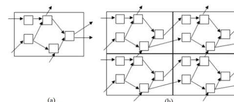
Figure 1. (Left) Example of a modular graph associated with four basic functions and five basic connections, three input points and three output points; (right) simplified description showing the acyclicity of the graph. Source: Nardi et al. (2009).
many practical cases the automatic production of code will not be totally optimal in terms of flexibility (e.g., when the direct model is updated frequently, one has to re-differentiate the whole code). These considerations motivated the devel-opment of a slightly different but complementary approach that focuses on the high-level structure of the numerical mod-els, embedding implementation details inside simple enti-ties that can be easily updated. This has led to the develop-ment of the YAO assimilation software at LOCEAN/IPSL (https://skyros.locean-ipsl.upmc.fr/~yao/).
YAO is based on the decomposition of a numerical model into elementary modules interconnected by directional links. On the one hand, the structure of the model (variables, de-pendencies. . . ) is described as a graph structure. On the other hand, the details of the physics are coded inside C/C++ basic modules that are ideally simple. The user can there-fore separate the “high-level” structure of the model from implementation details. It is also very easy to update a nu-merical code within this framework. Regarding the assimi-lation strategy, YAO computes the tangent linear and adjoint codes from the elementary Jacobians of each module (pro-vided by the user). Adjoint/cost function test tools are also available. Finally, YAO includes routines devoted to the clas-sical assimilation scenario (incremental form) and is inter-faced with the M1QN3 minimizer (Gilbert and LeMaréchal, 1989), which has been designed to minimize functions de-pending on a very large number of variables not subject to constraints. The algorithm implements a quasi-Newton tech-nique (L-BFGS) with a dynamically updated scalar or diago-nal preconditioner. It uses a line search to enforce global con-vergence; more precisely, the step size is determined by the Fletcher–Lemaréchal algorithm and realizes the Wolfe con-ditions.
3.3 Graph formalism
In YAO, a numerical model must be described as an ensem-ble of modules related by connections in order to form a graph. Let us define more precisely the main components of the graph.
– A module is a basic entity of computation, representing a deterministic (but possibly nonlinear) function trans-forming an input vector into an output vector. A module
Figure 2. (a)Example of a modular graph with five modules, as-sumed representative of the pointwise equations of a given model;
(b)partial view of the replication of the graph in space. Each ele-mentary graph with five modules is associated with one grid point. Source: Nardi et al. (2009).
is viewed graphically as a node of the graph; the sizes of the vectors correspond to the number of input and output connections associated with the node.
– A basic connection is an oriented link relating two nodes of the graph. Most basic connections usually rep-resent the transmission of the output of one module taken as input by another one.
The external context is the ensemble of data input and out-put points used as external data by a whole graph at a spe-cific level of abstraction. Basic connections can link a data input point located in the external context to one or several module(s) (for instance, modules needing the specification of some initial conditions, boundary conditions or model pa-rameters). Inversely, the global outputs of the model link a module to a data output point located in the external context. The modular graph is the ensemble of the modules and of their connections. It must be acyclic so that a topological order may be defined on the nodes of the graph (i.e., if there is connectionFp→Fq, thenFpshould be computed before
Fq)(see Fig. 1).
Typically, a modular graph describes the equations govern-ing the system of interest and each physical variable appear-ing in the governappear-ing equations is associated with a specific module. However, supplementary modules can also be de-fined to represent temporary variables required to simplify computations for complex equations. The user has gener-ally to specify modules at a single point (i, j, k, t) of space (i, j, k) and time (t) and the dependency on space–time loca-tions (e.g.,i+1,j−1,k,t−1) of the discretized variables taken as inputs. From the local description of the equations, YAO is able to build a model on a given space domain and on a given number of time steps by automatically replicating the local graph in space–time (cf. Fig. 2).
Now, we will see that the usefulness of the graph modu-lar approach is reinforced when the Jacobian matrix of each basic function is known. For a basic function F such that y=F(x), the Jacobian matrixFrelates a perturbation of the inputs to the associated perturbation of outputs: dy=Fdx. Since the Jacobian of a composition of functions is the prod-uct of the elementary Jacobians, the tangent linear model as-sociated with a modular graph may also be obtained by pass-ing the graph in the same topological order.
The “lin-forward” algorithm is the following.
1. Initialize the external context data input points with a perturbation dxi (around a given linearization point).
2. Pass the modules in topological order and propagate the perturbation.
3. Estimate the perturbation output dy on output data points in the external context of the graph.
Following this procedure, YAO can emulate the global tangent-linear model from elementary Jacobians. In the same manner, a backward algorithm may be defined for adjoint computations. From Eq. (1), it may be shown that the global adjoint will be retrieved by back-propagating the graph, with a few adjustments not detailed here (see Nardi et al., 2009, for more details on the “backward” algorithm). This prop-erty is the basis of the semi-automatic adjoint computation by YAO.
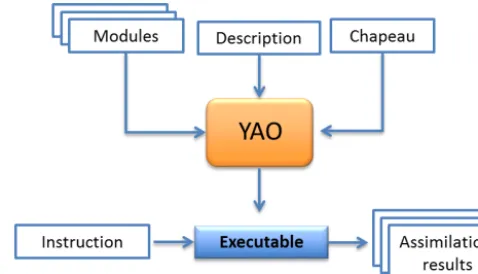
An implementation of a variational assimilation procedure with YAO follows the structure represented in Fig. 3. The YAO compiler builds an executable file following the scheme presented in Fig. 3. This file is independent of the assimila-tion instrucassimila-tions. The executable file reads these instrucassimila-tions from an instruction file. Due to the graph structure of the model and its adjoint, it is easy to modify the model and its adjoint, e.g., by updating some adequate modules; one can systematically obtain the updated global direct model and the global adjoint.
As mentioned in the Introduction, this paper gives access to a compiled version of SECHIBA-YAO and allows one to perform some assimilation experiments related to the control of the 10 most influent internal parameters of SECHIBA by observing the land surface temperature. YAO is a free soft-ware that gives the opportunity to modify the SECHIBA code provided in this paper.
3.4 Development of SECHIBA-YAO
The implementation of SECHIBA in YAO starts with the def-inition of the modular graph describing the dynamics of the model (see Appendix A). Elementary processes and intercon-nections between modules are defined in order to represent the computation flow in the model. The modular graph was built as follows.
– Every component of the original code was carefully studied line by line directly.
Figure 3.Structure of a project in YAO. The software generates an executable program from input modules, hat and description files. The generated program reads an instruction file to perform assimi-lation experiments.
– A list of inputs and outputs for each subroutine was made for every routine of SECHIBA. This permits one to know exactly the information flow in the model. – A second zoom in the subroutines was made in order to
understand the internal dynamics of the code. This is the last step in the modular graph definition. When studying the subroutines, their complexity was reduced by break-ing the different steps into simpler elements. The idea is to have a scalable code. Uncoupled modules give more independence when changing part of the model. Cohe-sive modules help to understand the model.
– The original six subroutines in the SECHIBA-Fortran code are split into 130 modules by the SECHIBA-YAO modular graph, corresponding to every process modeled by SECHIBA and to a number of transitional modules serving as auxiliary computing.
– It is important to mention that every variable and sub-routine name was kept as in the original model. If a user or developer of SECHIBA-Fortran sees the implemen-tation in YAO, he will find his way easily.
3.4.1 Direct model
After defining the modular graph in YAO, the second step in the SECHIBA-YAO implementation is the coding of the direct model and the derivatives of the modules. Every mod-ule is represented as a source file and the different processes attributed to the module are implemented inside the source file, allowing a better control of the physics; i.e., any change in the physics could be made easily.
3.4.2 Module derivatives
line-by-line based on the forward computing, in order to ob-tain the Jacobian matrix of the module, or they can also be produced routinely, using an automatic differentiation tool (for example, Tapenade; Hascoet and Pascual, 2013). For SECHIBA-YAO, the derivative process was made line-by-line. The outputs are derived with respect to every input. YAO generates automatically, based on these derivatives, the tangent linear and adjoint model.
Nevertheless, the derivative process introduced errors re-lated to the coding process, to inexact derivatives (e.g., ex-pressions that were not differentiable). In order to reduce it to a minimum number of bugs, the adjoint of the model was validated (as it was made with the direct model). This guar-antees the accuracy when performing assimilation. The vali-dation of the adjoint model is presented in Sect. 4.1.
4 Data assimilation experiments
In this section we present several experiments that have been realized using the SECHIBA-YAO system. They were de-signed to control the 11 most influential internal parameters of SECHIBA when we assimilate the land surface tempera-ture (LST).
In order to deal with non-dimensional control parameters with the same order of magnitude, preprocessing has been applied. The control parameters were first divided into two groups. The first group includes physical parameters, which have a physical dimension. In the present work, these param-eters were normalized by dividing them by their prior val-ues in order to control non-dimensional parameters. In such a way, given that the prior value is the true value (in the case of twin experiments), a value of 1 for these parameters indicates that the control parameter has been correctly reconstructed. The second group corresponds to physical parameters that are multiplied by a “multiplicative factor”, which is dimen-sionless (Verbeeck et al., 2001). The multiplying factors are the control variables of the second group and are set to 1 at the beginning of the assimilation process. The normalization process on the one hand and the use of multiplicative factors on the other hand allow us to deal with numbers of the same order of magnitude, which facilitates the comparison of the sensitivity of the different control variables in the assimila-tion process.
In the following, all variables are supposed to be prepro-cessed, so they are normalized and centered around 1.
The model inner parameters are the following (see Ta-ble 1): rsolcste is a numerical constant involved in the soil
resistance to evaporation. This parameter limits the soil evap-oration, so the greater its value, the lower the evaporation; humcste, mxeau and mindrain are related to soil water
pro-cesses: the higher their values, the more water will be avail-able in the model reservoir, affecting water transfers and es-pecially evapotranspiration; dpucsterepresents the soil depth
in meters. The other parameters are multiplicative factors;
they all have a value equal to 1:krveg, which is used in the
calculation of the stomatal resistance, limits the transpiration capacity of leaves; the greater its value, the lower the transpi-ration;kemiscontrols the soil emissivity used to compute land
surface temperature. This parameter takes part in the net ra-diation calculation which determines the energy balance be-tween incoming and outgoing surface fluxes;kalbedoweights
the surface albedo, which is defined as the reflection coeffi-cient for shortwave radiation;kcondandkcapatake part in the
thermal soil capacity and conductivity, both involved in the computation of the soil thermodynamics, and kz0 weights the roughness height, which determines the surface turbulent fluxes. Since the control parameters are normalized, we ap-ply a perturbation which is of the form of a random noise limited up to 50 % of the true parameter whose value is 1, so the perturbed value belongs to [0.5, 1.5]. If the control pa-rameter values posterior to the assimilation process are close to 1, it means that the assimilation was successfully achieved. Differences between the values retrieved and the prior values represent relative errors in the parameter estimation posterior to assimilation.
In order to show the benefit of data assimilation in SECHIBA, we conducted several experiments using SECHIBA-YAO. Prior to the assimilation process, different scenarios were defined for the tests (Table 3). A scenario makes reference to the experimental conditions. It includes the definition of the vegetation functioning type (PFT), the type of observation to be assimilated, the observation sam-pling, the time samsam-pling, the atmospheric forcing file, the subset of control parameters, the assimilation window size and the time of the year to start the assimilation. The differ-ent scenarios were calculated using the adjoint model for sev-eral typical conditions of the two FLUXNET sites selected. The dates presented in this paper are representative of sunny days in summer or winter, with no perturbation coming from clouds and without rainfall events. In Eq. (4), we takeRas the identity matrix, which means that we assume the errors of the observations are uncorrelated. The next section explains the scenarios for the different experiments performed in this work.
4.1 Variational sensitivity analysis
Table 1.SECHIBA inner parameters used in this work. There are five inner parameters involved in the model estimations that are controlled, plus six multiplicative factors, all equal to 1.
Parameter Description Prior value Unit
rsolcste Evaporation resistance 33 000 S m−2 humcste Water stress {5,2} m−1 mxeau Maximum water content 150 Kg m−3 mindrain Diffusion between reservoirs 0.001 S m−2 dpucste Total depth of soil water pool 2 m
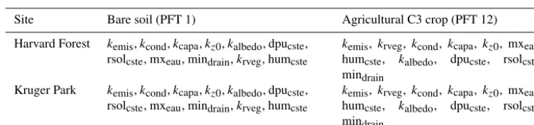
Table 2. Sensitivity analysis results. Parameter hierarchy according to each site and vegetation fraction. The parameters are ranked by decreasing sensibility.
Site Bare soil (PFT 1) Agricultural C3 crop (PFT 12)
Harvard Forest kemis,kcond,kcapa,kz0,kalbedo, dpucste, rsolcste, mxeau, mindrain,krveg, humcste
kemis, krveg, kcond, kcapa, kz0, mxeau, humcste, kalbedo, dpucste, rsolcste, mindrain
Kruger Park kemis,kcond,kcapa,kz0,kalbedo, dpucste, rsolcste, mxeau, mindrain,krveg, humcste
kemis, krveg, kcond, kcapa, kz0, mxeau, humcste, kalbedo, dpucste, rsolcste, mindrain
2008). This method is really local and the information pro-vided is related to a definite point in space. The values of the inner parameters (Table 1) and multiplicative factors (all equal to 1) represent the initial values where the experiments have been conducted. Because humcsteis related to
vegeta-tion type, in this work only the values for PFT 1 (5 m−1) and PFT 12 (2 m−1) are considered.
The sensitivity analysis was performed for a subset of inner parameters related to the energy and water physical processes on bare soil (PFT 1) and agricultural C3 crop (PFT 12), in order to quantify the role of the vegetation in the land surface temperature parameters’ sensitivity. The land functional types are useful for distinguishing the dif-ferent soil types. In the present case we used the agricul-tural C3 grass type whose parameters are Vcmax, opt
(op-timal maximum RuBisCO-limited potential photosynthetic capacity)=90 mol/m−2s−1; Topt (optimum photosynthetic
temperature)=27.5+0.25 Tl◦C; Tl (function of multian-nual mean temperature for C3 grasses); maxLAI(maximum
leaf area index (LAI) beyond which there is no allocation of biomass to leaves)=6;zroot(exponential depth scale for
root length profile)=0.25 m; leaf (prescribed leaf albedo)= 0.18;h(prescribed height of vegetation)=0.4 m; Ac (criti-cal leaf senescence)=150 days;Ts(weekly temperature
be-yond which leaves are shed if the seasonal temperature trend is negative)=10◦C; andH
s(weekly moisture stress beyond
which leaves are shed)=0.2.
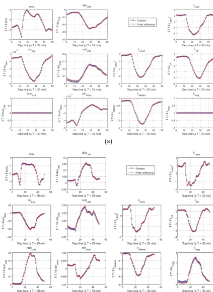
The work was done on a daily basis, in order to observe the diurnal variations of sensitivities. At each half-hour time step, model outputs are computed. At each time step, a gradi-ent is computed in order to have the updated gradigradi-ent value. As we make the assumption that the errors in prior values
are very large in comparison with errors in observations, we discard the background term in the cost function (defined in Sect. 2). This simplification is valid as soon as the system is overdetermined (i.e., the number of control parameters is smaller than the number of observations). The initial values of the parameters (before optimization) are those of Table 1. We recall that for numerical purposes, the control parame-ters have been normalized in order to have the same order of magnitude (i.e., equal to 1). Calculations were performed for both FLUXNET sites considered in this work.
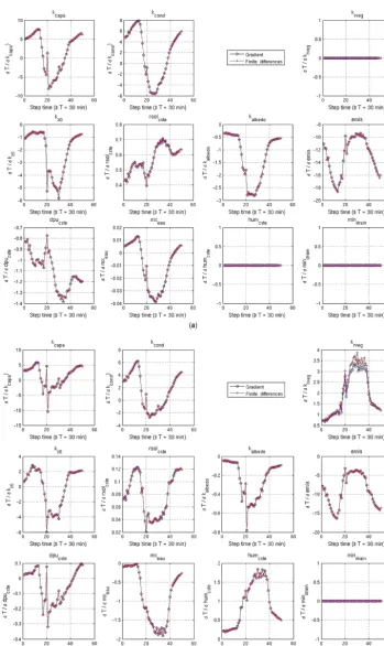
Figure 4 compares, for 28 August 1996 at Harvard Forest, the sensitivities computed for each control parameter with both finite differences and model gradients. Bare soil results are presented in Fig. 4a. The agricultural C3 crop scenario is illustrated in Fig. 4b. The efficiency of the adjoint calculation is first demonstrated in these plots, because the 11 desired parameter sensitivities are obtained in a single integration, whereas it takes 11 runs of the model to compute the same quantity using finite differences. By using the same method-ology, sensitivity curves were computed at FLUXNET site Kruger Park (Fig. 5). The comparison between sensitivity analysis done using the adjoint and using finite differences shows a very good agreement between the two methods for both sites. The diurnal characteristics of the parameter sensi-tivities with a maximum around noon in phase with the diur-nal variation of solar radiation are clearly visible.
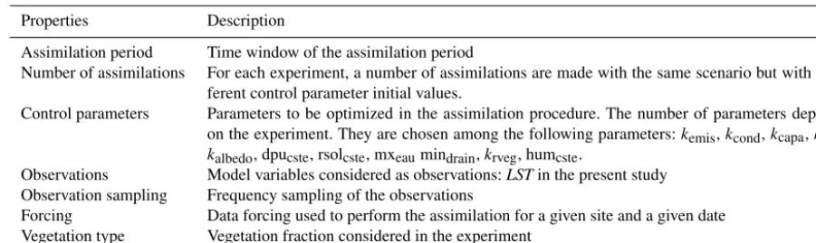
Table 3.Scenario properties and description.
Properties Description
Assimilation period Time window of the assimilation period
Number of assimilations For each experiment, a number of assimilations are made with the same scenario but with dif-ferent control parameter initial values.
Control parameters Parameters to be optimized in the assimilation procedure. The number of parameters depend on the experiment. They are chosen among the following parameters:kemis,kcond,kcapa,kz0, kalbedo, dpucste, rsolcste, mxeaumindrain,krveg, humcste.
Observations Model variables considered as observations:LSTin the present study Observation sampling Frequency sampling of the observations
Forcing Data forcing used to perform the assimilation for a given site and a given date Vegetation type Vegetation fraction considered in the experiment
that have the largest influence on the land surface tempera-ture estimate. Clearly kemis is the most influential
parame-ter in the calculation of land surface temperature, regardless of the climatology used and vegetation fraction. In addition, mindrainis the least influential parameter for all scenarios.
The parameters kcapa, kcond, kzo andkalbedo are the most
influential in bare soil conditions, afterkemis. In the presence
of vegetation, several sensitivities change radically:krveg
be-comes the most important multiplicative factor after kemis;
the factorkalbedois less sensitive compared to its influence in
the bare soil case and mxeauis more sensitive, given that less
water is available when a fraction of vegetation is present. The other parameters show equivalent sensitivity values re-gardless of the scenario. For humcsteandkrveg, sensitivities
are equal to 0 for bare soil, because these parameters affect surface temperature only in the presence of vegetation.
Parameters with persistent positive sensitivity are rsolcste,
krveg and humcste. Parameters with persistent negative
sen-sitivity are kz0,kalbedo and emis. The sign of the gradients
reflects the positive or negative feedback on the surface tem-perature of the processes involved. For example, the parame-ters involved in the evapotranspiration processes present neg-ative sensitivities because a reduction of (or an increase in) the evapotranspiration will lead to an increase (or a decrease) in the land surface temperature when the soil water content is sufficient.
Transpiration processes influence directly the land surface temperature in the presence of vegetation and are the dom-inant processes at the studied sites. Therefore krveg has a
higher sensitivity thankcond,kcapaandkalbedo. For bare soil,
by contrast, the dominant processes are those related to the soil thermodynamics, explaining whykcapa,kcond andkemis
are the most sensitive parameters.
In general, sensitivities are higher in bare soil conditions for the control parameters, except for mindrain and mxeau.
Since mindrain is not sensitive to the land surface
tempera-ture, this parameter is no longer controlled. Only the 10 most influential parameters are used in the following sections.
The next section presents the different assimilation exper-iments that we have performed using the SECHIBA-YAO software.
4.2 Twin experiments
Twin experiments permit one to check the robustness of the variational assimilation method by assimilating synthetic data. First the direct model is run with a set of parameters Ptrue (the initial conditions) in order to produce pseudo ob-servations of land surface temperature LST. Then Ptrue is randomly noised to obtain Pnoise. Assimilations of land sur-face temperature LST were then performed in the model run with Pnoise as new initial conditions for the control param-eters during several days (most of the time, 1 week), lead-ing to a new set of optimized parameters denoted as Passim. Passim is then compared to Ptrue in order to estimate the performances of the assimilation process. Five different as-similation experiments were performed. These experiments are available in the distributed version of SECHIBA-YAO. 4.2.1 Definition of experiments
The 10 most sensitive parameters are considered in the twin experiments (all the above parameters except mindrain). We
present hereinafter the results obtained with different assim-ilation realizations. Each assimassim-ilation experiment was con-ducted by perturbing the initial conditions of the control pa-rameters with a uniform distribution random noise reaching 50 % of the parameter nominal values. This procedure per-mitted us to obtain the relative errors of the control param-eters and the root mean square error (RMSE) of the model fluxes, based on their value before and after the assimilation process.
ex-Figure 4.Comparisons for 28 August 1996 at Harvard Forest of the sensitivities obtained for each control parameter with both the finite differences and the model gradients computed with the adjoint model. Sensitivity analysis results for PFT 1 are in(a)and for PFT 12 in
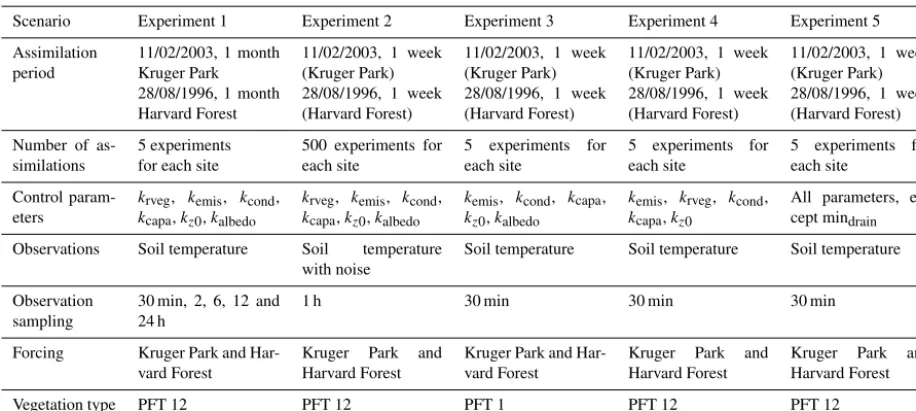
Table 4.Characteristics of the scenarios for each of the twin experiments.
Scenario Experiment 1 Experiment 2 Experiment 3 Experiment 4 Experiment 5
Assimilation period
11/02/2003, 1 month Kruger Park 28/08/1996, 1 month Harvard Forest
11/02/2003, 1 week (Kruger Park) 28/08/1996, 1 week (Harvard Forest)
11/02/2003, 1 week (Kruger Park) 28/08/1996, 1 week (Harvard Forest)
11/02/2003, 1 week (Kruger Park) 28/08/1996, 1 week (Harvard Forest)
11/02/2003, 1 week (Kruger Park) 28/08/1996, 1 week (Harvard Forest)
Number of as-similations
5 experiments for each site
500 experiments for each site
5 experiments for each site
5 experiments for each site
5 experiments for each site
Control param-eters
krveg, kemis, kcond,
kcapa,kz0,kalbedo
krveg, kemis, kcond,
kcapa,kz0,kalbedo
kemis, kcond, kcapa,
kz0,kalbedo
kemis, krveg, kcond,
kcapa,kz0
All parameters, ex-cept mindrain
Observations Soil temperature Soil temperature
with noise
Soil temperature Soil temperature Soil temperature
Observation sampling
30 min, 2, 6, 12 and 24 h
1 h 30 min 30 min 30 min
Forcing Kruger Park and
Har-vard Forest
Kruger Park and Harvard Forest
Kruger Park and Har-vard Forest
Kruger Park and Harvard Forest
Kruger Park and Harvard Forest
Vegetation type PFT 12 PFT 12 PFT 1 PFT 12 PFT 12
Table 5.Sampling frequencies for Experiment 1.
Test Sampling Observations Observation number frequencies per day per month
1 30 min 48 1440
2 2 h 24 720
3 6 h 4 120
4 12 h 2 60
5 24 h 1 30
cept for Experiment 1, where the time step varies. All exper-iments presented in this work use Harvard Forest and Kruger Park as forcing. For each experimental setting, five different assimilation realizations were made, except for Experiment 2, where 500 independent assimilations were run. The mean errors are presented in Table 4.
– In Experiments 1 and 2, the six most sensitive param-eters are controlled. In both cases the vegetation type is PFT 12. In Experiment 1 several observation as-similation samplings are tested, going from 30 min up to 24 h. During 1 month, five independent assimilation tests were run for each observation sampling. In Exper-iment 2, a weighted random noise was introduced in the observations, going from 10 up to 50 % of the true value of the observation. Both Experiments 1 and 2 use con-stant perturbations of the control parameters (50 % of its prior value for Experiment 1 and 10 % for Experiment 2) in order to assess the impact of varying the observa-tion sampling and the noise in the observaobserva-tions. – In Experiment 3 the five most sensitive parameters
ac-cording to the sensitivity analysis (Table 2) were con-trolled in bare soil conditions (PFT 1) at the Harvard
Forest and Kruger Park sites. In this experiment the noise added on the prior values is 50 %.
– In Experiment 4 the five most sensitive parameters for each PFT were controlled in the conditions of agricul-tural C3 (PFT 12), according to the sensitivity analysis (Table 2), in the Harvard Forest and Kruger Park sites. In doing so, we were able to assess the effect of the vegetation fraction on the assimilation system. In ad-dition, taking only the most sensitive parameters in the control set permitted us to increase the assimilation per-formances, given that the more the observed variable is sensitive to a parameter, the easier the minimization process finds its optimal value, consequently reducing the estimation error. In this experiment the noise added on the prior values is 50 %.
– In Experiment 5, all parameters, except mindrain, were
controlled (since mindrainhas no impact on the land
sur-face temperature estimation), during a week in Harvard Forest and Kruger Park.
Comparing Experiment 5 with Experiments 3 and 4 allows us to study the impact of taking a larger number of control pa-rameters on the assimilation process. In addition, we want to test whether LST observation provides enough information to constrain all the model parameters at the same time and whether we can hope to improve all model state variables. In this experiment the noise added on the prior values is 50 %. 4.3 Results
4.3.1 Effect of the observation sampling
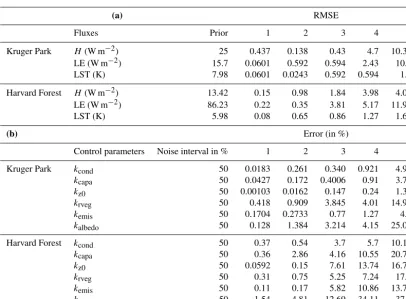
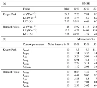
Table 6.Results of Experiment 1 using the Harvard Forest and Kruger Park sites.(a)The first two columns give the computed fluxes prior to the assimilation. The last five columns present the RMSE (prior-estimated) for each run.(b)The first two columns give the noise interval (in %) introduced for each control parameter with respect to the initial value of 1. The last five columns present the relative error in % in the control parameters for the five sampling frequencies reported in Table 5.
(a) RMSE
Fluxes Prior 1 2 3 4 5
Kruger Park H (W m−2) 25 0.437 0.138 0.43 4.7 10.34 LE (W m−2) 15.7 0.0601 0.592 0.594 2.43 10.8 LST (K) 7.98 0.0601 0.0243 0.592 0.594 1.9
Harvard Forest H (W m−2) 13.42 0.15 0.98 1.84 3.98 4.08 LE (W m−2) 86.23 0.22 0.35 3.81 5.17 11.95
LST (K) 5.98 0.08 0.65 0.86 1.27 1.61
(b) Error (in %)
Control parameters Noise interval in % 1 2 3 4 5
Kruger Park kcond 50 0.0183 0.261 0.340 0.921 4.96
kcapa 50 0.0427 0.172 0.4006 0.91 3.77
kz0 50 0.00103 0.0162 0.147 0.24 1.34
krveg 50 0.418 0.909 3.845 4.01 14.97
kemis 50 0.1704 0.2733 0.77 1.27 4.4
kalbedo 50 0.128 1.384 3.214 4.15 25.01
Harvard Forest kcond 50 0.37 0.54 3.7 5.7 10.14
kcapa 50 0.36 2.86 4.16 10.55 20.74
kz0 50 0.0592 0.15 7.61 13.74 16.73
krveg 50 0.31 0.75 5.25 7.24 17.8
kemis 50 0.11 0.17 5.82 10.86 13.74
kalbedo 50 1.54 4.81 12.69 34.11 37.8
varying the observation frequency leads to varying the num-ber of observations available. Each test was labeled with a number. This number serves as a reference to compare the different results. Table 5 presents the several tests we con-ducted as well as their initial conditions. For example, in Test 4, only two observations per day are taken at noon and at midnight. In Test 5, we have one observation per day, taken at noon, and so on.
Prior and final errors before and posterior to the assimila-tion process are presented in Table 6 for the Kruger Park and Harvard Forest sites. The columns represent the different as-similations performed with different frequency sampling in the observations. Five independent assimilations were done for each test. Table 6 reports the mean value of the perfor-mances of the assimilation system. Even though small errors were found for the different tests, we do notice that the as-similation system is sensitive to the observation sampling.
The contribution of the observations is demonstrated by an improvement in the optimization when increasing the fre-quency of observations, both for the controlled parameters and the computed fluxesHand LE that are major outputs of the model. The final error values in the different tests increase by a factor of 10 when reducing the sampling frequency.
4.3.2 Effect of random noise in the observation
Experiment 2 aims at studying the impact of introducing a random noise in the synthetic observations. The random noise follows a normal distribution with zero mean and vari-ance 1. The perturbed observations are computed using the following equation:
LST∗=LST+]amp·ϕ, (7)
Table 7.Experiment 2 (different amplitudes of random noise in the observations) using the Harvard Forest and Kruger Park sites. We present the mean values for 500 experiments:(a)the first two columns give the computed fluxes prior to the assimilation. The last three columns present the RMSE (prior minus estimated) for a given level of noise added to the observations (10, 30, 50 %).(b)The first two columns give the noise interval (in %) introduced for each control parameter with respect to the initial value of 1. The last three columns present the mean error in % in the control parameters for different levels of noise (10, 30, 50 %) added to the observations (LST).
(a) RMSE
Fluxes Prior 10 % 30 % 50 %
Kruger Park H (W m−2) 24.7 7.26 7.81 8.32 LE (W m−2) 4.06 3.78 3.9 6.22
LST (K) 7.12 0.019 4.48 6.23
Harvard Forest H (W m−2) 25 5.92 11.13 24.01 LE (W m−2) 15.7 4.77 14.04 15.05
LST (K) 7.98 0.046 1.42 2.59
(b) Mean error (%)
Control parameters Noise interval in % 10 % 30 % 50 %
Kruger Park kcond 10 4.5 4.9 11.12
kcapa 10 1.51 3.35 14.9
kz0 10 3.24 3.99 4.09
krveg 10 6.91 10.1 11.5
kemis 10 2.79 3.14 4.08
kalbedo 10 1.12 2.01 3.02
Harvard Forest kcond 10 0.83 4.32 7.6
kcapa 10 4.47 9.05 9.21
kz0 10 3.85 4.5 7.3
krveg 10 1.36 7.01 8.04
kemis 10 2.39 3.62 6.47
kalbedo 10 1.02 2.58 7.85
We note in Table 7a and b that the parameter restitution is degraded when adding random noise to the observations. This shows that the sensitivity of the assimilation system to the noise affecting the LST observations is quite high. When increasing the amplitude of the error, the various errors ob-tained for the three tests not only suggest the need to take into account the quality of the observations in the model, but also the fact that the parameters are not affected in the same way by the data uncertainties. However, perturbations are still limited and a deeper exploration should be performed to assess the impact on the assimilation performance of noisy observations.
4.3.3 Effect of the control parameter set size
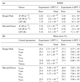
The RMSE errors of the assimilations for Experiments 3, 4 and 5 are presented in Tables 8 and 9, corresponding to the Harvard Forest and Kruger Park sites. For all the experiments the noise added on the parameters was 50 %. In Experiment 3 for PFT 1, the mean errors in the retrieved values for all the control parameters are on the order of 10−8. Regarding the LST retrieval, the mean RMSE ranges from 4.82 K prior to assimilation to 2.1×10⁻⁵K after the assimilation process.
The same behavior is observed for the different model fluxes. Both FLUXNET sites used as forcing have more or less the same behavior with regards to the error reduction. In Experi-ment 4 for PFT 12, similar results were observed. The assim-ilation process permits the reduction of the parameter errors for both sites and both PFTs used (Table 8b). In Experiment 5, the relative value of the RMSE with respect to the syn-thetic measurements, for LST, LE andH, is reduced at both FLUXNET sites. The same results hold for the mean relative error of the control parameters.
as-Table 8.Results for Experiments 3 (PFT 1) and 4 (PFT 12). RMSE of model fluxes(a)and parameter relative errors(b)before and after the assimilation process on FLUXNET Harvard Forest and Kruger Park.
(a) RMSE
Fluxes Experiment 3 (PFT 1) Experiment 4 (PFT 12)
Prior Final Prior Final
Kruger Park H(W m−2) 4.22 4.1×10⁻¹² 2.18 2.4×10⁻⁹ LE (W m−2) 4.51 2.6×10⁻⁴ 6.86 3.2×10⁻⁵ LST (K) 7.15 2.3×10⁻⁵ 2.32 8.3×10⁻⁹ Harvard Forest H(W m−2) 2.33 2.2×10⁻¹² 1.52 1.5×10⁻¹⁰ LE (W m−2) 2.45 7.3×10⁻⁴ 8.34 2.4×10⁻⁶ LST (K) 5.14 4.3×10⁻⁵ 1.37 7.1×10⁻¹⁰
(b) Mean error (%)
Control parameters Experiment 3 (PFT 1) Experiment 4 (PFT 12)
Prior Final Prior Final
Kruger Park kcond 25.4 3.17×10⁻¹¹ 27.3 6.37×10⁻⁶ kcapa 25.3 3.1×10⁻¹¹ 27.3 5.64×10⁻⁶ kz0 25.1 6.7×10⁻¹¹ 26.3 7.97×10⁻⁵
krveg – – 28.1 2.76×10⁻⁶
kemis 25.8 3.01×10⁻¹¹ 27.5 6.08×10⁻⁵
kalbedo 25.9 5.2×10⁻¹¹ – –
Harvard Forest kcond 24.1 5.58×10⁻⁵ 26.9 5.85×10⁻⁶ kcapa 25.4 5.57×10⁻⁶ 25.8 7.84×10⁻⁷ kz0 24.4 1.27×10⁻⁵ 25.8 7.84×10⁻⁷
krveg – – 22.1 8.31×10⁻⁶
kemis 25.5 5.71×10⁻⁴ 24.2 5.96×10⁻⁷
kalbedo 23.4 1.99×10⁻⁴ – –
similation of this variable in order to optimize these parame-ters is not efficient.
5 Discussion and conclusion
In this study the adjoint of SECHIBA was implemented us-ing adjoint semi-generator software denoted YAO. The land surface temperature gradients with respect to each control pa-rameter were computed by SECHIBA-YAO, which permitted us to carry out a sensitivity analysis of the parameter influ-ence on the synthetic LST estimation on the one hand and to conduct several assimilation experiments on the other hand.
The first contribution of this paper was the sensitivity anal-ysis results. They showed exactly which parameters of the model are the most sensitive and have to be controlled during the assimilation process. However, it is important to mention that sensitivity analysis depends on the region, the forcing, the PFT, and the time period (hour and day), among other fac-tors. Once the parameter hierarchy was set, twin experiments were performed for different scenarios, aiming at testing the robustness of the assimilation scheme.
The second contribution of this work is that we showed the usefulness of the variational data assimilation of LST (land surface temperature) for improving the SECHIBA parameter estimations. LST assimilation has the potential to improve the LSM parameter calibration, by adjusting them properly during the control process. In a forecasting approach, this can be valuable, due to the fact that the simulation can be more reliable, since the model parameters are fitted on actual measurements. Improvement in the fluxes computed by the model after the assimilation of LST was demonstrated. Twin experiments showed the power of variational data assimila-tion to improve the model parameter estimaassimila-tion. Different experiments conducted for different scenarios and forcing sites were successfully accomplished, meaning that a reduc-tion in the fluxes errors was obtained by introducing infor-mation given by the LST synthetic observations. In addition, the influence of the size of the control parameter set in the assimilation performance was proven.
Table 9.Results for Experiment 5 (PFT 12). RMSE of model fluxes
(a)and parameter relative errors(b) before and after the assimi-lation process, on the FLUXNET Harvard Forest and Kruger Park sites.
(a) RMS
Fluxes Experiment 5 (PFT 12)
Prior Final
Kruger Park H(W m−2) 30.4 2.1
LE (W m−2) 34.1 3.1
LST (K) 3.12 3.2×10⁻¹
Harvard Forest H(W m−2) 41.5 5.4
LE (W m−2) 24.1 2.3
LST (K) 5.2 5.1×10⁻¹
(b) Mean error (%)
Control parameters Experiment 5 (PFT 12)
Prior Final
Kruger Park kcond 23.4 2.3×10⁻¹
kcapa 26.6 2.1×10⁻¹
kz0 22.2 1.5×10⁻¹ krveg 25.9 3.1×10⁻¹
kemis 24.5 2.3×10⁻¹ kalbedo 23.8 1.8×10⁻¹
mxeau 26.3 6.8×10⁻¹
humcste 22.4 1.9×10⁻¹
dpucste 25.6 3.2×10⁻¹
rsolcste 23.1 1.9×10⁻¹
Harvard Forest kcond 25.1 3.30×10⁻¹ kcapa 26.7 2.61×10⁻¹
kz0 25.4 1.79×10⁻¹ krveg 27.5 2.8×10⁻¹
kemis 26.3 2.1×10⁻¹ kalbedo 24.7 2.37×10⁻¹
mxeau 25.8 7.34×10⁻¹
humcste 25.2 2.7×10⁻¹
dpucste 24.2 2.2×10⁻¹
rsolcste 25.4 2.36×10⁻¹
system to retrieve the prior value of the control parameters with a high accuracy. After presenting the different experi-ments, some aspects of data assimilation arise when analyz-ing the results. The first one concerns the presence of several local minima due to the nonlinearity of the SECHIBA model. Second, we have also shown a significant improvement in the assimilation performances when the sampling frequency of observations is increased, as evaluated in Experiment 1. This suggests that the ability of the model to be constrained de-pends, among other things, on the observation frequency. By decreasing the number of observations, the control parame-ter adjustment is less accurate, and the assimilation proce-dure estimates variables with a larger error. Therefore it can be verified that if we have more LST observations, the as-similation system will fit the parameters better so improved estimations are obtained.
Finally, we observe a strong dependence between the qual-ity of observations and the parameter restitution, as shown in Experiment 2. It seems crucial to take into account the un-certainty in the observations, because they do not affect the assimilation performance in the same way when estimating each parameter in the minimization process. If we compare Experiments 1 and 2 (Tables 6 and 7), it is clear that the noise on the observations dramatically increases the mean error on the computed fluxesL and H; the LSTs that are assimilated, are retrieved with a better accuracy. The intro-duction of a regularization term on the parameters could be used to mitigate this problem. Constraining parameters and weighting observations according to their confidence in the minimization phase can be modeled through the introduction in the cost function of the variance–covariance error matrices (backgroundBand observationR). It is an important aspect to consider for assimilating real observations.
Adding extra parameters to the control set increases the complexity of the cost function. By taking into consideration the results of assimilation of LST when controlling the 10 most sensitive parameters (Experiment 5), we could see that, after having made several assimilation runs, LST does not provide enough information to constrain the parameter set, in order to improve the estimation of the SECHIBA parameters. In the case of controlling all parameters we cannot hope to improve the estimation of all model parameters unless we assimilate additional observations or we add a background term in the cost function.
Assimilation with the YAO approach permits the imple-mentation of different assimilation scenarios in a very flex-ible way when performing different twin experiments: the control parameters and the observed variables (once the ad-joint code has been generated), the assimilation windows, the observation sampling, the time sampling and other different features can be changed easily.
A distributed version of SECHIBA-YAO code and several examples with different scenarios are available at a GitHub dedicated site. YAO can be downloaded upon request at https://skyros.locean-ipsl.upmc.fr/~yao/. Direct use of this software will allow one to perform other experiments using different physical conditions or even to change several equa-tions of the model.
6 Code and data availability
The distributed version of SECHIBA-YAO provides an op-portunity for scientists to perform their own assimilation. The distributed version allows the control of the five most influent internal parameters of SECHIBA, depending on the vegetation type. In addition, LST or satellite brightness tem-perature can be used as observations.
it in a local repertory and run themakefilein order to build a local executable. Documentation and two instruction files are available in order to guide the user towards their own implementation. Users can modify the forcing file, the ini-tial date to the assimilation, the parameter value and their perturbation if needed. The assimilation frame (1 week), the step time (30 min), the observed variable (land surface tem-perature), the control parameters (only five) and other initial parameters are imposed. If a user wants to have access to a full modifiable version, the YAO software has to be installed (https://skyros.locean-ipsl.upmc.fr/_yao/).
Appendix A: SECHIBA-YAO
The version of SECHIBA implemented in YAO includes the two-layer hydrology of Choisnel (1977), mentioned in Sect. 2. SECHIBA original code is implemented in a modu-lar scheme with a set of well-defined routines, independent in its processes and with a single entry point (a main routine handling the rest of the functionalities).
A set of prognostic variables is defined for each module and its assignation depends on the forcing conditions, phys-ical phenomena, etc. SECHIBA can work coupled with the other components of ORCHIDEE (STOMATE and LPJ) or it can be used offline, as it was used in this work. Once SECHIBA is coded in YAO, it can be easily coupled with the other modules of ORCHIDEE.
In SECHIBA, the different routines were originally coded in the Fortran language and can be run at any resolution and over any region of the globe. The version of SECHIBA im-plemented in YAO is denoted SECHIBA-YAO and follows the Fortran code. In its present form, it can only be run at one point at a time.
ORCHIDEE uses MODIPSL and IOIPSL in its in-ternal processes (see http://forge.ipsl.jussieu.fr/igcmg/wiki/ platform/documentation for more information). Developed at IPSL, the first one is a set of scripts allowing the extrac-tion of a given configuraextrac-tion from a computing machine and the compilation of the specific machine configuration com-ponents. MODIPSL is the tree that will host models and tools for configuration. IOIPSL helps to manage the variables state history, variable normalization, and file lecture, among oth-ers.
The main routines in SECHIBA-Fortran are presented in Fig. A1. These are also the routines considered in the YAO implementation of the model. First, DIFFUCO computes the diffusion and plant transpiration coefficients based on the atmospheric conditions, solar fluxes, dry soil height, soil moisture stress and fraction of vegetation. ENERBIL corre-sponds to the energy budget module. Surface energy fluxes related to the soil are computed, based on atmospheric con-ditions, radiative fluxes, resistances, surface-type fractions and surface drag. HYDROLC is the hydrological budget module, taking as inputs the rainfall, snowfall, evaporation components, soil temperature profile and vegetation distribu-tion. CONDVEG helps in the computation of the vegetation conditions. The thermodynamics of the model is computed in THERMOSOIL, based on a seven-layer soil profile. Fi-nally, SLOWPROC computes the soil slow processes. When SECHIBA is decoupled from STOMATE, this module also deals with the LAI evolution.
The different SECHIBA components are interconnected as shown in Fig. A2. The output of the different modules serves as inputs for the next one, thus resulting in an interde-pendency among modules to be considered when modeling SECHIBA-YAO.
Figure A1.SECHIBA subroutines and their corresponding outputs. Source: Benavides Pinjosovsky (2014).
Acknowledgements. This work used eddy covariance data ac-quired by the FLUXNET community and in particular by the following networks: AmeriFlux (U.S. Department of Energy, Biological and Environmental Research, Terrestrial Carbon Program and AfriFlux) and the global FLUXNET project (http://daac.ornl.gov/FLUXNET/fluxnet.html). A special thanks to M. Crepon from LOCEAN for his active participation in the revi-sion of this article. P. Peylin and F. Chevalier are acknowledged for fruitful discussions. We thank also F. Maignan for her continuous support in the use of the ORCHIDEE model, and M. Berrondo for the assistance in writing this article.
Edited by: J. Kala
Reviewed by: B. Coudert, R. Mechri, and A. Kallel
References
Aubinet, M., Vesala, T., and Papale, D.: Eddy Covariance: A Prac-tical Guide to Measurement and Data Analysis, Springer Atmo-spheric Sciences Editions, United States of America, 2012. Baldocchi, D., Falge, E., Gu, L., Olson, R., Hollinger, D.,
Running, S., Anthoni, P., Bernhofer, C., Davis, K., Evans, R., Fuentes, J., Goldstein, A., Katul, G., Law, B., Lee, X., Malhi, Y., Meyers, T., Munger, W., Oechel, W., Paw, K. T., Pilegaard, K., Schmid, H. P., Valentini, R., Verma, S., Vesala, T., Wilson, K., and Wofsy, S.: FLUXNET: a new tool to study the temporal and spatial variability of ecosystem-scale carbon dioxide, water vapor, and energy flux densi-ties, B. Am. Meteorol. Soc., 82, 2415–2434, doi:10.1175/1520-0477(2001)082<2415:FANTTS>2.3.CO;2, 2001.
Bateni, S. M., Entekhabi, D., and Jeng, D. S.: Variational as-similation of land surface temperature and the estimation of surface energy balance components, J. Hydrol., 481, 143–156, doi:10.1016/j.jhydrol.2012.12.039, 2013.
Benavides Pinjosovsky, H. S.: Variarional data assimilation in the land surface model ORCHIDEE using YAO, Earth Sciences, Université Pierre et Marie Curie – Paris VI, available at: http: //www.theses.fr/2014PA066590, last access: 14 September 2014. Bischof, C. H., Bouaricha, A., Khademi, P. M., and Mor, J. J.: Com-puting gradients in large-scale optimization using automatic dif-ferentiation, Informs J. Comput., 9, 185–194, 1997.
Castelli, F., Entekhabi, D., and Caporali, E.: Estimation of sur-face heat flux and an index of soil moisture using adjoint-state surface energy balance, Water Resour. Res., 35, 3115–3125, doi:10.1029/1999WR900140, 1999.
Choisnel, E.: Le bilan d’Énergie et le bilan hydrique du sol, Paris, Météorologie Nationale, 1977.
d’Orgeval, T., Polcher, J., and Li, L.: Uncertainties in modelling future hydrological change over west africa, Clim. Dynam., 26, 93–108, doi:10.1007/s00382-005-0079-3, 2006.
Ducoudré, N., Laval, K., and Perrier, A.: SECHIBA, a new set of parametrizations of the hydrologic exchanges at the land/atmosphere interface within the LMD atmospheric gen-eral circulation model, J. Climate, 6, 248–273 doi:10.1175/1520-0442(1993)006<0248:SANSOP>2.0.CO;2, 1993.
Dufresne, J. L., Foujols, M. A., Denvil, S., Caubel, A., Marti, O., Aumont, O., Balkanski, Y., Bekki, S., Bellenger, H., Benshila, R., Bony, S., Bopp, L., Braconnot, P., Brockmann, P., Cadule,
P., Cheruy, F., Codron, F., Cozic, A., Cugnet, D., de Noblet, N., Duvel, J. P., Ethe, C., Fairhead, L., Fichefet, T., Flavoni, S., Friedlingstein, P., Grandpeix, J. Y., Guez, L., Guilyardi, E., Hauglustaine, D., Hourdin, F., Idelkadi, A., Ghattas, J., Jous-saume, S., Kageyama, M., Krinner, G., Labetoulle, S., Lahel-lec, A., Lefebvre, M. P., Lefevre, F., Levy, C., Li, Z. X., Lloyd, J., Lott, F., Madec, G., Mancip, M., Marchand, M., Masson, S., Meurdesoif, Y., Mignot, J., Musat, I., Parouty, S., Polcher, J., Rio, C., Schulz, M., Swingedouw, D., Szopa, S., Talandier, C., Terray, P., Viovy, N., and Vuichard, N.: Climate change projections us-ing the IPSL-CM5 Earth System Model: from CMIP3 to CMIP5, Clim. Dynam., 40, 2123–2165, doi:10.1007/s00382-012-1636-1, 2013.
Evensen, G.: The ensemble Kalman filter: Theoretical formula-tion and practical implementaformula-tion, Ocean Dynam., 53, 343–367, doi:10.1007/s10236-003-0036-9, 2003.
Friedlingstein, P., Joel, G., Field, C. B., and Fung, I.: To-ward an allocation scheme for global terrestrial carbon mod-els, Glob. Change Biol., 5, 755–770, doi:10.1046/j.1365-2486.1999.00269.x, 1999.
Ghent, D., Kaduk, J., Remedios, J., and Balzter, H.: Data assimilation into land surface models: The implications for climate feedbacks, Int. J. Remote Sens., 3, 617–632, doi:10.1080/01431161.2010.517794, 2011.
Giering, R. and Kaminski, T.: Recipes for Adjoint Code Construction, ACM Trans. Math. Softw., 24, 437–474, doi:10.1145/293686.293695, 1998.
Gilbert, J. C. and LeMaréchal, C.: Some numerical experiments with variable-storage quasi Newton algorithms, Maths. Program, 45, 407–435, doi:10.1007/BF01589113, 1989.
Harrison, D. E., Chiodi, A. M., and Vecchi, G. A.: Effects of surface forcing on the seasonal cycle of the eastern equatorial Pacific, J. Mar. Res., 67, 701–729, doi:10.1357/002224009792006179, 2009.
Hascoët, L. and Pascual, V.: The Tapenade Automatic Differentia-tion tool: principles, model, and specificaDifferentia-tion, Research Report Nro 7557. Project Team Tropics, INRIA, France, 2012. Hascoet, L. and Pascual, V.: The Tapenade Automatic
Differentia-tion tool: principles, model, and specificaDifferentia-tion, ACM TransacDifferentia-tions on Mathematical Software, Association for Computing Machin-ery, 39, doi:10.1145/2450153.2450158, 2013.
Huang, C., Li, X., and Lu, L.: Retrieving land surface temper-ature profile by assimilating MODIS LST products with en-semble Kalman filter. Cold and Arid Regions Environmen-tal and Engineering Research Institute, CAS, Lanzhou, China, doi:10.1016/j.rse.2007.03.028, 2003.
Ide, K., Courtier, P., Ghil, M., and Lorenc, A.: Unified Nota-tion for Data AssimilaNota-tion: OperaNota-tional, Sequential and Vari-ational, Special Issue, J. Meteorol. Soc. Jpn., 75, 181–189, doi:10.1.1.47.2607, 1997.
Krinner, G., Viovy, N., Noblet-Ducoudre, N. de, Ogee, J., Polcher, J., Friedlingstein, P., Ciais, P., Sitch, S., and Prentice, I. C.: A dynamic global vegetation model for studies of the coupled atmosphere-biosphere system, Global Biogeochem. Cy., 19, 1, doi:10.1029/2003GB002199, 2005.
Lahoz, W. and Khattatov, B.: Data Assimilation Making Sense of Observations, Springer Editions, 2010.
Le Dimet, F.-X. and Talagrand, O.: Variational Algorithms for Anal-ysis and Assimilation of Meteorological Observations: Theoret-ical Aspects, Dynamic Meteorology and Oceanography, 38, 97– 110, doi:10.1111/j.1600-0870.1986.tb00459.x, 1986.
Nardi, L., Sorror, C., Badran, F., and Thiria, S.: YAO: A Software for Variational Data Assimilation Using Numerical Model, Com-putational Science and its Applications – ICCSA 2009, Interna-tional Conference, 5593, 2, 621–636, 2009.
Pipunic, R. C., Walker, J. P., and Western, A.: Assimilation of remotely sensed data for improved latent and sensible heat flux prediction: A comparative synthetic study, 19th Interna-tional Congress on Modelling and Simulation, Perth, Australia, doi:10.1016/j.rse.2007.02.038, 2008.
Reichle, R., Kumar, S., Mahanama, S., Koster, R. D., and Liu, Q.: Assimilation of satellite-derived skin temperature observations into land surface models, J. Hydrometeorol., 11, 1103–1122, doi:10.1175/2010JHM1262.1, 2010.
Ridler, M., Sandholt, I., Butts, M., Lerer, S., Mougin, E., Timouk, F., Kergoat, L., and Madsen, H.: Calibrating a soil–vegetation–atmosphere transfer model with remote sens-ing estimates of surface temperature and soil surface mois-ture in a semi-arid environment, J. Hydrol., 436–437, 1–12, doi:10.1016/j.jhydrol.2012.01.047, 2012.
Robert, C., Blayo, E., and Verron, J.: Comparison of reduced-order, sequential and variational data assimilation methods in the trop-ical Pacific Ocean, Ocean Dynam., 56, 624–633, 2007.
Saltelli, A.: Sensitivity Analysis, John Wiley & Sons Edi-tion, United States of America, doi:10.1007/s10236-006-0079-9, 2008.
Sitch, S., Smith, B., Prentice, I. C., Arneth, A., Bondeau, A., Cramer, W., Kaplan, J. O., Levis, S., Lucht, W., Sykes, M. T., Thonicke, K., and Venevsky, S.: Evalua-tion of ecosystem dynamics, plant geography and terres-trial carbon cycling in the LPJ dynamic global vegetation model, Glob. Change Biol., 9, 161–185, doi:10.1175/1525-7541(2002)003<0728:EVEKFF>2.0.CO;2, 2003.
Svendsen, H.: The effect of clear sky radiation on crop surface tem-perature determined by thermal thermometry, Agr. Forest Mete-orol., 50, 239–243, doi:10.1016/0168-1923(90)90057-D, 1990. Talagrand, O.: The use of adjoint equations in numerical modeling
of the atmospheric circulation, Automatic Differentiation of Al-gorithms: Theory, Implementation, and Application, edited by: Griewank, A. and Corliess, G., SIAM, 169–180, 1991.