Source apportionment using LOTOS-EUROS: module description and evaluation

(1)

Geosci. Model Dev., 6, 721–733, 2013 www.geosci-model-dev.net/6/721/2013/ doi:10.5194/gmd-6-721-2013

EGU Journal Logos (RGB)

Advances in

Geosciences

Open Access

Natural Hazards

and Earth System

Sciences

Open Access

Annales

Geophysicae

Open Access

Nonlinear Processes

in Geophysics

Open Access

Atmospheric

Chemistry

and Physics

Open Access

Atmospheric

Chemistry

and Physics

Open Access Discussions

Atmospheric

Measurement

Techniques

Open Access

Atmospheric

Measurement

Techniques

Biogeosciences

Open Access Open Access

Biogeosciences

Discussions

Climate

of the Past

Climate

of the Past

Discussions

Earth System

Dynamics

Earth System

Dynamics

Discussions

Geoscientific

Instrumentation

Methods and

Data Systems

Open Access

_{Geoscientific}

Instrumentation

Methods and

Data Systems

Geoscientific

Model Development

Geoscientific

Model Development

Discussions

Hydrology and

Earth System

Sciences

Open Access

Hydrology and

Earth System

Sciences

Ocean Science

Discussions

Solid Earth

Discussions

The Cryosphere

Discussions

Natural Hazards

and Earth System

Sciences

Open Access

Discussions

Source apportionment using LOTOS-EUROS: module description

and evaluation

R. Kranenburg, A. J. Segers, C. Hendriks, and M. Schaap

TNO, P.O. Box 80015, 3508 TA, Utrecht, the Netherlands

Correspondence to: R. Kranenburg ([email protected])

Received: 30 October 2012 – Published in Geosci. Model Dev. Discuss.: 28 November 2012 Revised: 26 April 2013 – Accepted: 7 May 2013 – Published: 3 June 2013

Abstract. To design effective mitigation strategies, the origin

of emissions which produce air pollutants needs to be known. Contributors to air pollutants can be emission sources, like road traffic or industry, but also be more specified to emis-sion from one location or from a specified time. Chemistry transport models can be used to assess the origin of air pol-lution across a large domain. However, in traditional sim-ulations the information on origin is lost and brute force scenario studies are performed to assess the origin. Alter-natively, one can trace the origin of air pollutants through-out a simulation using a labeling approach. In this paper we document and demonstrate a newly developed labeling mod-ule for the chemistry transport model LOTOS-EUROS which tracks the source allocation for all particulate matter compo-nents and precursor gases. Dedicated simulations confirmed that the new module functions correctly. The new module provides more accurate information about the source contri-butions than using a brute force approach with scenario runs as the chemical regime remains unchanged. An important ad-vantage of the new module is the reduction of computation costs and analysis work associated with the calculations. The new module was applied to assess the origin of particulate ni-trate across the Netherlands. Averaged across the Dutch ter-ritory, the main contributions to nitrate are derived from road and non-road transport as well as power plants. Overall, only one-fifth of the concentration derived from sources located inside the country. The new technology enables new research directions as improved information on pollution origin is de-sired for policy support as well as scientific applications.

1 Introduction

(2)

Hence, they implicitly contain the information to perform a source apportionment. Numerous studies have employed a brute force approach to gain insight in source contributions. In these studies scenario runs are used reducing the emis-sions of sources under investigation and comparing the dif-ferences to the base case (e.g. Lane et al., 2007). Although the computational burden is large, this approach provides a good insight into inert species. However, in case of species involved in atmospheric chemistry, a negative impact on the source apportionment results may occur as perturbing emis-sions may cause non-linear effects. Presently, few models are equipped with modules to overcome these negative im-pacts on chemical reactive species. Most divide the PM com-ponents into source-specific species that are tracked sepa-rately through the model (e.g. McHenry et al., 1992; Ying and Kleeman, 2006). These approaches are capable of accu-rately tracking the source contribution for secondary species. However, the computational burden remains as large as us-ing a scenario approach limitus-ing their use for a large num-ber of sources. Note, tagging methods have also been devel-oped for ozone by Emmons et al. (2012), Butler et al. (2011), Grewe et al. (2010) and Wang et al. (2009). In these meth-ods the model description is extended with duplicate tracers and chemical reactions. Yarwood et al. (2004) and Wagstrom et al. (2008) present the Particulate Source Apportionment Technology (PSAT) algorithm within CAMx, combining the capability of accurately dealing with secondary species with limited CPU demand. With PSAT the concentration of the species is modelled as before, but next to this the fractional contribution of all sources is kept track of through all pro-cesses. CAMx incorporates detailed process descriptions, but requires a large computational time to perform simulations over long time periods. Hence, applications to the full Eu-ropean domain do not exist. We developed a source appor-tionment model for the operational CTM LOTOS-EUROS (Schaap et al., 2008) to be able to study the origin of par-ticulate matter in Europe in more detail. In this paper we document, validate and demonstrate the new source appor-tionment module inspired by the PSAT approach. We ap-ply the source apportionment system to study the origin of ammonium nitrate in the Netherlands. Ammonium nitrate is the most important component of particulate matter in the Netherlands (Weijers et al., 2011). In the Netherlands am-monium nitrate levels rise more than proportionally with to-tal PM (Weijers et al., 2011), which has also been observed in other countries (Putaud et al., 2010). We focus on nitrate as it is a product of complex chemistry and its precursor orig-inates from multiple source sectors. The source apportion-ment for nitrate is part of a larger effort to assess the ori-gin of PM in the Netherlands as reported by Hendriks et al. (2013). In this paper we first present a short overview of the LOTOS-EUROS model (Sect. 2). Second, a detailed descrip-tion of the labeling source appordescrip-tionment technique is given (Sect. 3. Next, the results of a technical validation to ensure a proper functioning of the system for the different processes

are presented (Sect. 4), with special attention to the chem-istry in Sect. 5. Also, the application aimed to establish the origin of nitrate in the Netherlands is shown (Sect. 6). The paper is concluded with a summary of the main results and a short discussion on the benefits of the developed module.

2 The LOTOS-EUROS chemistry transport model

The model employed in this study is the 3-D chemistry trans-port model LOTOS-EUROS, which is aimed at the simu-lation of air pollution in the lower troposphere. The model is of intermediate complexity in the sense that the relevant processes are parameterized in such a way that the com-putational demands are modest enabling hour-by-hour cal-culations over extended periods of several years within ac-ceptable CPU time. The current master domain of LOTOS– EUROS is bound at 35◦ _{and 70}◦_{N and 30}◦_{W and 60}◦_E.

The model projection is normal longitude–latitude and the standard grid resolution is 0.50◦longitude×0.25◦ latitude, approximately 25 km×25 km. The actual domain for a sim-ulation can be set as long as it falls within the master domain as specified above. In addition, it is possible to increase or de-crease the resolution up to factor 4. In the vertical, the model extend to 3.5 km above sea level and uses the dynamic mix-ing layer approach to determine the model vertical structure. This means that on top of a 25 m surface layer a well-mixed boundary layer is assumed. The height of the mixing layer is obtained from the ECMWF meteorological input data used to drive the model. The height of the reservoir layers is deter-mined by the difference between ceiling (3.5 km) and mixing layer height. Both layers are equally thick with a minimum of 50 m. In a few cases, when the mixing layer extends near or above 3500 m, the top of the model exceeds the 3500 m according to the above-mentioned description. The tion in all directions is handled with a monotonic advec-tion scheme (Walcek and Aleksic, 1998). Gas phase chem-istry is described using the TNO CBM-IV scheme, which is a condensed version of the original scheme (Whitten et al., 1980). Hydrolysis of N2O5is described explicitly (Schaap et al., 2004). Cloud chemistry is described following Banzhaf et al. (2011). Aerosol chemistry is represented using ISOR-ROPIA2 (Nenes et al., 1998). The dry deposition in LOTOS-EUROS is parameterized following the well-known resis-tance approach following the EDACS system (Erisman et al., 1994), including a compensation point approach for ammo-nia (Wichink Kruit et al., 2012). The aerodynamic resistance is calculated for all land use types separately. Below cloud scavenging is described using simple scavenging coefficients for gases (Schaap et al., 2004) and particles (Simpson et al., 2003).

(3)

annual total into monthly totals. This value is multiplied by a factor for the day of the week (i.e. Monday, Tuesday, etc.) and finally with a factor for the hour of the day (local time). The LOTOS-EUROS model includes a biogenic emission routine based on detailed information on tree species over Europe (Koeble and Seufert, 2001). The emission algorithm is described in Schaap et al. (2009) and is very similar to the simultaneously developed routine by Steinbrecher et al. (2009). Sea salt emissions are described using M˚aertensson et al. (2003) and Monahan et al. (1986) for the fine mode and coarse mode, respectively.

The LOTOS-EUROS model has participated in several in-ternational model intercomparison studies addressing ozone (Hass et al., 1997; Van Loon et al., 2007; Solazzo et al., 2012a) and particulate matter (Cuvelier et al., 2007; Hass et al., 2003; Stern et al., 2008; Solazzo et al., 2012b) and shows comparable performance to other European models. The LOTOS-EUROS model shows a systematic underesti-mation of PM of about 40 %. This is mainly due to the miss-ing process descriptions for secondary organic aerosols in the model. For the secondary inorganic aerosols the model shows a much smaller underestimation, while the temporal correla-tion is about 0.6 to 0.8.

3 Source apportionment module

3.1 Overview

To track the origin of the modelled concentrations for differ-ent tracers, a source apportionmdiffer-ent module for the LOTOS-EUROS was developed. The method is developed for the LOTOS-EUROS version 1.8 and can be generally used in later versions. Using a labeling technique the new modules calculate the contribution of specified sources for all model grid cells and time steps. In this calculation the contributions per label are calculated as fractions of the total tracer concen-tration. As the fractions must add up to one for mass conser-vation, all processes that are sources and sinks of mass within the model must be accounted for in the source apportionment module, including initial and boundary conditions. The cal-culations to track the source contributions differ per process; the processes in the model can be categorized in four groups:

– Emissions

– Anthropogenic emissions – Natural emissions

– Transport processes

– Advection – Diffusion – Adjustment – Sedimentation

– Removal processes

– Dry deposition – Wet deposition

– Chemistry

– Gas phase chemistry – Aerosol chemistry

For each of these processes the calculations are described be-low.

3.2 Emissions

The specification of the labels to track throughout the model simulations is done in the emission routine. In principle, the definition of the labels is very flexible and any kind of al-location is possible as long as the required detail is present in the input data. For example, emissions from road trans-port, from a specific country during daylight can be labelled. As one is mainly interested in the source contribution of the anthropogenic sources, the natural emissions (sea salt, bio-genic non-methane volatile organic compounds (NMVOC) and windblown dust) are treated separately and obtain a sep-arate label. In the current application and system environ-ments, the number of labels is restricted to 35. With this amount of labels, the runtime and the output will still be fea-sible.

For each hour in the simulations the base emission data containing the annual average emission per sector and coun-try for each grid cell is processed and added into the emis-sion array using the sector dependent time profiles. During this processing the source contributions are also accounted for in the array fremis(l). This array contains the emission of each source of interest (labelled byl) as a fraction of the total emission. During each time stepn, the concentration changes due to all emissions (cf) are added to the existing concentra-tionscn−1and the new source allocation frn(l) is updated by a straight forward weighted average of existing and concen-tration change:

f rn(l)=

f rn−1(l)·cn−1+f remis(l)·cf

cn .

In the equation above frn(l)and frn−1(l)are the new and the

old fractions for label l. The total old and new concentra-tions are given bycn−1andcn,while the emitted mass flux converted to a concentration change is given by cf. In the model, concentrations are in volume mixing ratios (ppb) for the gaseous tracers and in mass concentrations (µg m3) for the particles.

3.3 Transport processes

(4)

the Walcek scheme, the concentration fluxes through the cell edges are calculated based on the fluxes between the two nearest upwind and the nearest downwind cells. The fluxes are limited by the maximum and minimum concentration of the two surrounding cells. Due to this application, the advec-tion process is slightly non-linear.

For the update of the source allocation, the mass fluxes between all cells are passed to the labeling routine. The new source allocation in each cell is calculated with the source allocation of the remaining concentration and the sum over the source allocations of the influx(es)Fin of the cell. The remaining concentration is the old concentrationcn−1minus the sum of all the outfluxes, which has the same source allo-cation as the old concentration. The new source alloallo-cation is then the following:

f rn(l)=

f rn−1(l)·(cn−1−Fout_V·1t)+ K P k=1

Fin,k(l)·1t

V cn

.

Here, Fout is the total mass or volume outflux (µg s−1 or m3s−1), while V is the volume (m3) of the cell. The total number of neighbor cells isK. The mass or volume influx (µg s−1or m3s−1) per label is defined as

Fin(l)=f rn−1(l)in·Fin.

The fractionsf rn−1(l)in for the mass influxFin are taken

from the comparing donor cell.

All other processes that govern one-dimensional transport, i.e. diffusion, sedimentation and adjustment are implemented following the same approach. The influxes are stored and with those the new source allocation is calculated. The pro-cess adjustment accounts for the concentration changes due to the adaption of the vertical layering structure as a conse-quence of the rise and fall of the mixing layer.

3.4 Wet and dry deposition

Wet and dry deposition are important sinks in the model. As it is assumed that each molecule of a species has the same probability to be deposited, the source apportionment for the concentration arrays does not change. A complication is as-sociated with the treatment of the re-emission of ammonia which is possible as the model includes the bi-directional surface-atmosphere exchange (Wichink Kruit et al., 2012). Here we assume that the exchange is fast and the source allo-cation of this emitted ammonia is given the same alloallo-cation as the concentration in air. Alternatively, one could store the source allocation of the ammonia deposition fluxes and use these for the re-emission flux. Given the short atmospheric lifetime and the dominant impact of agriculture for ammo-nia, we feel that both approaches would yield very similar results.

3.5 Gas phase chemistry

The gas phase chemistry in LOTOS-EUROS is described us-ing a CBM4 mechanism. We aim to provide a source attri-bution that is valid for the current atmospheric conditions. As a consequence, the labeling process is only implemented for chemical active tracers with an N, C or an S atom. These atoms are conserved and are traceable. This means that four oxidants (OH, H2O2, HO2and O3) and two operator species (XO2and XO2N) are not traced.

Recent studies to the origin of ozone use a tagging method with duplicate tracers and reactions (Grewe, 2004; Butler et al., 2011; Dahlmann et al., 2011; Grewe et al., 2012). For this purpose one has to assume a NOx of volatile organic compounds (VOC) limited chemical regime. With the same assumptions the methodology outlined below could also be used for ozone. As the chemical limitation varies across Eu-rope, a sensible application is not straightforward and there-fore not pursuit here.

The following differential equation is solved to calculate the new concentrations of all species.

dc

dt =cp+clc

Here,clcontains the loss rates (s−1) andcpcontains the pro-duction rates (ppb s−1). Further,crepresents the concentra-tion of a single tracer (ppb). This system is solved with a numerical implicit method, with the following result:

cn=

cn−1+dt·cp 1+dt·cl .

In herecn−1andcnare the new (at timet+dt) and old (at timet) concentrations for each species.

The main assumption for the labeling for the chemistry is that first the species are produced before their loss is taken into account. For the source allocation of each species it is necessary to keep track of the produced material as func-tion of its originating species containing the corresponding C, N or S atom. One of the main advantages in the chemi-cal scheme used in LOTOS-EUROS is that this information is easily available. From the solver the production rates split into origin of species are passed to the labeling routine us-ing a square production matrix Yp(ppb s−1) with the size of the number of labelled species. The columns indicate the re-acted species, while the rows contain the produced species. For example: the entry with column index of NO and row in-dex of NO2corresponds with the produced NO2out of NO, which is a composition of all production rates that deal with production of NO2 out of NO. In the labeling routine, the new source contributions are calculated with the following formula:

f rn(l)=f rn−1(l)·cn−1(l)+dt·f rn−1(l)·Yp cn−1+dt·cp

(5)

Here, f rn−1(l) and f rn (l) are the old and new frac-tions of labell, while cn−1 (l) is the old concentration for labell. Note that the first multiplication in the numerator is a vector–vector multiplication, which multiplies the entries of both vectors one by one. The second multiplication is a full matrix–vector multiplication, which are generally com-putationally expensive. As the matrix Ypis sparse, a special routine for sparse matrices is used to save computer time.

To illustrate the process we use the reaction of nitrogen dioxide with the hydroxyl radical as an example:

NO2 + OH → HNO3with ratek.

This reaction produces nitric acid (HNO3) and results in a loss of nitrogen dioxide (NO2). The reaction clearly illus-trates that the N-atom is conserved. This reaction will lower the NO2concentration but will not change the source appor-tionment of NO2as all NO2molecules have the same chance to react. The produced HNO3has the origin of NO2. The new concentration per label for HNO3(cn(HNO3, l)) is calculated as follows (only the reaction above is involved):

f rn(HNO3, l)=

cn−1(HNO3)·f rn−1(HNO3,l)+Yp(HNO3,NO2)·f rn−1(NO2,l) cn−1(HNO3)+cp(HNO3) .

With Yp(HNO3, NO2)=k·[NO2]·[OH]. The term Yp (HNO3, NO2)·f rn−1 (NO2, l) corresponds with the label specific production of HNO3from NO2. The termcp(HNO3) corresponds with the total produced HNO3. In the case with only one reaction, this term is equal to Yp(HNO3, NO2).

In the current implementation it is assumed that for the production of species with C, N or S atoms, the source ap-portionment is taken from the original species with the cresponding atom. This means that for reactions between or-ganic compounds and nitrogen oxides such as the oxidation of formaldehyde by the NO3 radical, the origin of the pro-duced HNO3 is taken from the that of NO3 while the ori-gin of the produced CO is taken from that of formaldehyde. The reactions forming and dissociating peroxy acetyl nitrate (PAN) are an exception to this rule as PAN combines both C and N atoms in a single molecule. It is an important reser-voir species and may be transported over quite a distance. At some point PAN will dissociate, but within the current implementation there is no way to keep track of the origi-nal N or C source contributions. Therefore, the source appor-tionment of the produced PAN is taken from both precursor species (C2O3 and NO2). For the dissociation reaction the normal procedure is followed. Consequently, this is the only way for sources without an N-emission to receive a small but non-zero contribution to the N-species. Note that the cur-rent implementation enables excluding the labeling of the C-atoms by limiting the Yp matrix to the inorganic chemistry only. This feature was implemented as an option as it gives a slightly more accurate source allocation for the inorganic

species and, more importantly, reduces computing time since the matrix vector multiplication is much smaller. In this study the full source apportionment is used.

3.6 Aerosol chemistry

The source apportionment of non-volatile aerosol compo-nents, such as sulfate and sodium nitrate, is straightforward and follows the approach outlined for the gas phase chem-istry. However, a different approach is taken for a semi-volatile component such as ammonium nitrate. The ther-modynamic equilibrium module ISORROPIA-II is used in LOTOS-EUROS to assess the partitioning between nitric acid (HNO3) and nitrate (NO3), as well as between ammo-nia (NH3) and the ammonium (NH4). In a thermodynamic equilibrium the exchange between the gas to aerosol phase is by definition equal. Though no net mass is exchanged, the constant exchange between the two phases will cause the ori-gin of the gas and aerosol phase to equalize. Hence, after the equilibrium calculation the source attribution of nitrate (am-monium) and nitric acid (ammonia) are averaged:

f rn(HNO3) = f rn(NO3) =

f rn−1(HNO3)·cn−1(HNO3)+f rn−1(NO3)·cn−1(NO3) cn−1(HNO3)+cn−1(NO3)

f rn(NH3) = f rn(NH4) =

f rn−1(NH3)·cn−1(NH3)+f rn−1(NH4)·cn−1(NH4) cn−1(NH3)+cn−1(NH4) .

4 Technical validation

The development and implementation of the labeling tech-nique was performed for each process at a time. The correct functioning of the code was evaluated with dedicated exper-iments. For the emission, vertical diffusion, deposition and adjust processes a simple experiment could be designed as their solution is refined to a single column and the processes are linear. For advection a more elaborate and indirect ex-periment was performed. Below we present the performance evaluation for these cases. Note, for the chemistry, the func-tioning of the module is illustrated in Sect. 5 as it is not pos-sible to give a technical validation.

4.1 Case 1: linear processes

To test the labeling technique for the linear processes emis-sion, deposition, diffuemis-sion, sedimentation and adjust, the LOTOS-EUROS model was run for the month of Jan-uary 2007, for primary PM components. These include:

– EC fine: Elemental Carbon in fine mode (ECf)

– PPM fine: Primary Particulate Matter in fine mode

(6)

– PPM coarse: Primary Particulate Matter in coarse mode

(PPMc)

The ECfemissions are estimated as a percentage of the fine mode primary PM (PPMf) emissions using sector dependent factors (Schaap et al., 2004). This approach enabled defining a simulation in which the ECfconcentration is calculated as a separate tracer and compared to a labelled ECffraction of the PPMfconcentration. Thus, within this simulation the ECf fraction of all primary PM components was labelled using five labels:

– Fraction ECf

– Fraction not ECf

– Boundary conditions (north, east, south and west

boundaries)

– Initial condition

– Aloft boundary condition (boundary on top of the

do-main)

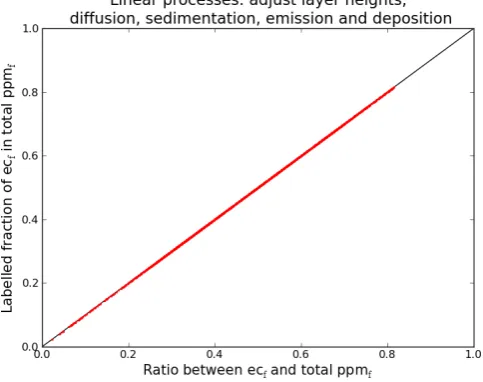
As the boundary and initial conditions were set to zero, their fraction should remain zero. Moreover, the fractions of ECffor components ECfand PPMcshould remain 1 and 0, respectively, which they did. The contribution of EC in PPMf should equal the ECfconcentration in the model. In Fig. 1, the results are shown for the combination of the linear pro-cesses in the model. The results show that the fractions of la-bel ECffor PPMffits perfectly on the ratio between ECfand PPMf. There are small deviations which are caused by the numerical precision in the computations. Tests using all lin-ear processes separately yields the same results. From these experiments it is clear that the source allocation routine for these processes functions correctly.

4.2 Case 2: advection

In the second performance test we add the advection process to the system. We perform an annual simulation for 2007 for a small domain centred around the Netherlands including the Netherlands, Belgium, northern France and the western part of Germany. Simulations were performed for the full year of 2007. The labels were defined to represent the geographical areas:

– Belgian emissions

– German emissions

– Dutch emissions

– Emissions from other countries or seas

– Boundary conditions

– Initial conditions

Fig. 1. Scatter plot of the ratio between fine elemental carbon (EC f) and total primary PM in the fine mode (PPM f) against the labelled fraction of EC f in PPM f. This scatter plot is valid for the linear processes: Adjust layer heights, vertical diffusion, sedimentation, emission and deposition.

– Aloft boundary condition

The results of this labeling simulation were compared to four scenario simulations in which only the one of the men-tioned regions emit their emissions. As the primary species are treated to be inert, the system is linear except for the ad-vection and a close resemblance is expected.

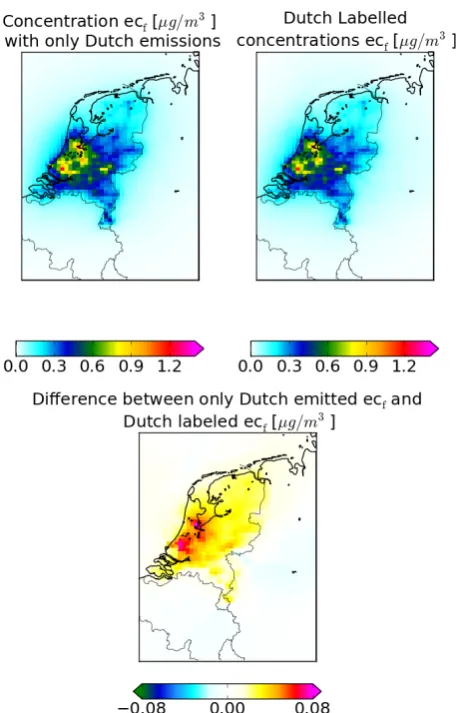
In Fig. 2 we present the results for the Dutch contribu-tion to the modelled EC concentracontribu-tion. The annual mean EC distribution for the scenario run containing Dutch emissions (upper left) closely resembles that of the Dutch labelled con-centrations for the full model simulation (upper right). The differences between the estimates for the Dutch EC contri-bution differs at most by 4 % (lower panel). These small dif-ferences are induced by the Walcek advection algorithm in which the fluxes through the cell edges are calculated as a weighted average of one downwind and two upwind cells. In case of scenario simulations with different concentrations gradients the fluxes through the cell edges will slightly dif-fer between the simulations. This becomes mostly visible around large source areas. Also the impact of the border is visible in the difference due to the steep concentration gradi-ent across the border in case of a scenario run. In a labeling simulation all sources are included and the impact of differ-ences in gradients are avoided. As such, one could argue that the labeling technique provides a more consistent approach than scenario simulations.

4.3 Computational cost

(7)

Fig. 2. Upper left: concentration elemental carbon in fine mode (EC f) resulting from a model simulation with only Dutch emis-sions. Upper right: concentration EC f from a full model simulation corresponding to the label on Dutch emissions. Lower: the differ-ence between those two simulations. These simulations are done with the linear processes and the non-linear advection process for the complete year 2006.

effort containingnscenarios. The computational time of sin-gle simulation using the source apportionment tool is larger than for a single scenario due to the additional bookkeeping and calculations. However, it is only a fraction of the total of all scenario runs. In Fig. 7 the computation time using the new tool as a fraction of the computation time forn sce-nario runs is given for both simulations with inert and chemi-cally active components. The graph shows that the computer time saved increases with the number of labels. For exam-ple, withn=24 labels and inert tracers one needs only about

17 percent of the computational time compared to 24 sce-nario runs. In case the full chemistry is added, the profit is somewhat smaller as the chemistry is the most expensive part in LOTOS-EUROS. Still, the computational costs with 24 labels are about a factor 4 lower than using scenario runs. The sharp decrease in run time for only a few labels can be

explained by the overhead cost. Within one run, the com-putational cost of reading and processing the input data is relatively large.

5 Illustration of the labeling approach for chemical active tracers

In principle, it is impossible to give a technical validation of the functioning of the labeling routine for a full chemistry simulation as the chemistry scheme is non-linear. Compar-ing a labelCompar-ing to a scenario simulation will show the impact of indirect effects through changes in oxidant levels and the change in pollutant levels. Hence scenario calculations can-not provide a real benchmark for the chemistry (Emmons et al., 2012; Grewe et al., 2012). Still, to illustrate the function-ing of the module, we compare a simulation in which we label a relatively small fraction (5 %) of the Dutch emissions to a scenario simulation with the same emission reduction on all anthropogenic sources. The simulations were performed for July 2006 with active photochemistry. Results are dis-cussed for three components with a different origin and life-time (carbon monoxide, methylglyoxal and nitrogen oxides). We first compare the results for carbon monoxide (CO) as its chemistry is relatively simple, it has a long life time and has strong anthropogenic sources. Hence, the impact of changes in chemical regime is expected to be small. Next, we com-pare the results of a reaction product from the degradation of non-methane volatile organic compounds (NMVOC) being methylglyoxal (MGLY). This species has a short life time and is largely determined by oxidation of biogenic VOC. Hence, the impact of the chemical regime is expected to be very large. Finally, we discuss NO and NO2as they behave typically due to the impact of the photo-stationary equilib-rium.

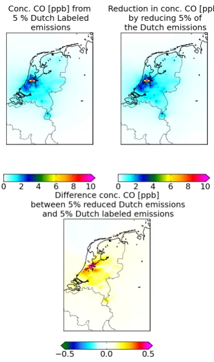
In Fig. 3 the labelled 5 % contribution (upper left) is com-pared to the impact of the 5 % emission reduction (upper right). Both simulations produce a CO contribution of about 2 ppb in the Randstad, with lower values in the more ru-ral part of the Netherlands and highest values in industrial-ized areas. The difference between both results (Fig. 3: lower panel) is an order of magnitude lower than the estimated 5 % contribution itself. The non-linearity in the chemistry (and the transport) provides a difference of about 2–10 % in the estimated Dutch contribution, which we consider to be rela-tively small. As the Netherlands is characterized by very high NOxemissions, the difference can be explained by a net in-crease in oxidant levels in the scenario simulation due to the decreasing impact of ozone titration.

(8)

Fig. 3. Upper left: concentration carbon monoxide from a full model simulation corresponding to 5 % of the Dutch emissions. Upper right: carbon monoxide concentrations from a full simulation mi-nus concentration from a simulation with 5 % reduced Dutch emis-sions. Lower: the difference between those two. These simulations are valid for the month July of 2006.

are not all the same. We expect that the change in chem-ical regime impacting all formation and destruction routes has a large impact on the estimated contribution based on the scenario. To validate this assumption a second simula-tion was performed with only a 5 % reducsimula-tion on the Dutch NMVOC emissions, keeping all other emissions the same. The lower right panel of Fig. 4 shows the concentration change for MGLY for this simulation. The results are much closer to the labelled simulation, both in magnitude and gra-dients. Differences are now at most 10 % and occur in regions where anthropogenic emissions are largest and non-linearity in the chemistry and its impact on the solver is expected to be largest. The close agreement provides confidence in the functioning of the source apportionment module. These re-sults also clearly illustrate the difference between source ap-portionment based on scenarios versus a labeling technique.

Fig. 4. Upper: concentration methylglyoxal (MGLY) from a full model simulation corresponding with the 5 % labelled Dutch emis-sions. Lower left: MGLY concentrations from a full simulation mi-nus concentration from a simulation with 5 % reduced Dutch an-thropogenic emissions. Lower right: MGLY concentrations from a full simulation minus concentration from a simulation with 5 % re-duced Dutch anthropogenic NMVOC emissions. These simulations are valid for the month July of 2006.

(9)

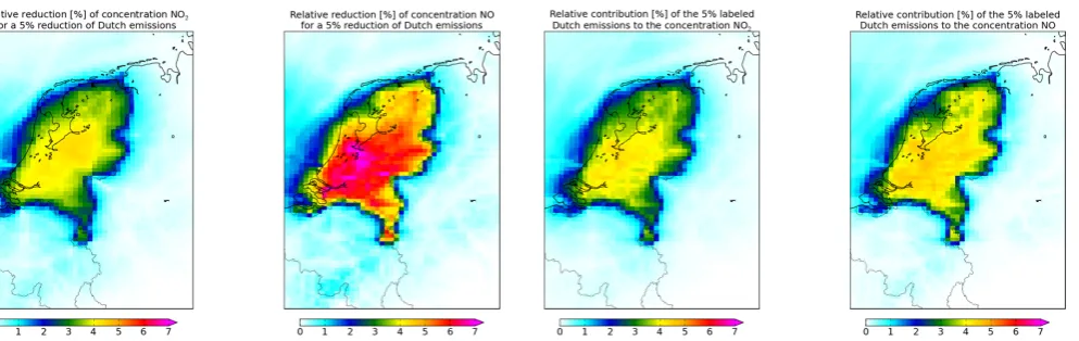
Fig. 5. Relative reduction of concentration NO2 (left) and NO (right) by a reduction of 5 % of the Dutch emissions. These sim-ulations are valid for the month July of 2006.

may not impact NO2but will impact NO to a larger extend. This feature is clearly visible in the scenario results. The case shows that the first reduction on NOxemissions will not be most effective to reduce NO2levels evidenced by the lower than 5 % impact on NO2. However, in a mixture of emission sources all contributions have the same probability to react. The labeling simulation therefore yields much closer values to 5 %, which is the actual anticipated result (Fig. 6). Again, these results show the functioning of the module and the ad-vantage it may have on a brute force study based on scenario studies.

6 Application to the origin of nitrate across the Netherlands

To demonstrate the potential applications of the source ap-portionment module, we provide an assessment of the ori-gin of particulate nitrate across the Netherlands. The major-ity of the nitrate in the Netherlands is present in the form of ammonium nitrate, whereas coarse mode (sodium) nitrate contributes a minor part (Weijers et al., 2011; Ten Brink et al., 1997). Both formation mechanisms are present in the LOTOS-EUROS model. Annual mean modelled concentra-tions underestimate the observed nitrate concentraconcentra-tions by about 20 %. Evaluation against daily particulate matter sam-ples (Hendriks et al., 2013) as well as hourly observations (Schaap et al., 2011) show that the model is able to capture the variability in time quite well. For a detailed discussion on the model performance and associated uncertainties we refer to these papers. Here, we present the source apportionment for nitrate obtained with a simulation in which labels were defined to track the national and foreign contributions of all SNAP level 1 emission sectors (20 in total). Note that the interpretation of the results was also made for all PM com-ponents and is presented in detail in Hendriks et al. (2013).

Fig. 6. Relative contribution of the 5 % labelled Dutch emissions to the total concentration of NO₂(left) and NO (right). These simula-tions are valid for the month July of 2006.

(10)

Fig. 7. Time efficiency of the labeling module with respect to the scenario approach. On the x-axis the number of labels (sources of interest) defined. On the y-axis the relative fraction of computation time with respect to the total computation time of all needed scenar-ios run (for each source of interest a separate scenario run).

not very fast, limiting the aerosol nitrate formation. However, when the air mass reaches the main land with intense am-monia emissions the formation ammonium nitrate becomes effective, explaining the maximum along the coast line.

The examples above show that system is able to track the origin of components with complex formation pathways. The system presently tracks the source contributions to oxidized (e.g. nitrogen oxides) and reduced (e.g. ammonia) nitrogen species separately. Hence, the origin of nitrate is not con-nected to that of ammonia, which is needed to form ammo-nium nitrate. Hence, ammoammo-nium nitrate is one of the few ex-amples where the interaction between the different labelled classes is important. The present approach that was chosen as the implementation is clear and results are easily explainable. An alternative could be to perform a post processing by at-tributing the mass of ammonium nitrate equally to the origin of ammonia and fine mode nitrate. As ammonia is derived more than 90 % from agriculture, the alternative approach shows that agriculture contributes almost half of the nitrate mass (Fig. 8), whereas the contributions of all other sectors are almost halved. Also, the national contribution increases as ammonia has a shorter lifetime than oxidized nitrogen. Hence, it advised to provide results for both approaches in future studies.

7 Conclusions

We have developed and demonstrated a new module to inves-tigate source contributions to modelled air pollutant distribu-tions. We feel that the labeling module provides more ac-curate information about the source contributions than using

Fig. 8. Contributions of Dutch, foreign, natural and boundary sources (left) and anthropogenic source sectors (right) to nitrate concentrations averaged over the Netherlands. The attribution is shown as a function of nitrate levels on the x-axis. The upper panels present the default source attribution. The lower panels present the source attribution corrected for the ammonium nitrate assumption

Fig. 9. Modelled source contributions of foreign non-road transport and Dutch road transport to nitrate concentrations (µg m−3)across the Netherlands.

(11)

so for most species and a reasonable number of sources in one simulation. In principle, the selection of sources is flex-ible and can be set by the modeller. An important advantage of the new module is the reduction computation costs as-sociated with the calculations. Not only the computer time is reduced, also the preparation of a labeling simulation re-quires less work than setting up N scenarios. Moreover, using a single emission database and model simulations reduces the amount of errors and recalculations. The new technology opened new research directions for, for example, the inter-pretation of monitoring and remote sensing data (Hendriks et al., 2013) as well as the derivation of source receptor ma-trices.

Acknowledgements. This study was partly funded by the 7th Framework Programme of the European Commission EnerGEO (see http://www.energeo-project.eu) and by the Dutch cooperation of model and data centers (NMDC).

Edited by: T. Butler

References

Banzhaf, S., Schaap, M., Kerschbaumer, A., Reimer, E., Stern, R., van der Swaluw, E., and Builtjes, P.: Implementation and eval-uation of pH-dependent cloud chemistry and wet deposition in the chemical transport model REM-Calgrid, Atmos. Environ., 49, 378–390,doi:10.1016/j.atmosenv.2011.10.069, 2011. Bobbink, R., Hicks, K., Galloway, J., Spranger, T., Alkemade, R.,

Ashmore, M., Bustamnte, M., Cinderby, S., Davidson, E., Den-temer, F., Emmett, B., Erisman, J-W., Fenn, M., Gilliam, F., Nordin, A., Pardo, L., and de Vries, W.: Global assessment of nitrogen deposition effects on terrestrial plant diversity: a syn-thesis, Ecol. Appl., 20, 30–59, doi:10.1890/08-1140.1, 2010. Butler, T. M., Lawrence, M. G., Taraborelli, D., and Lelieveld, J.:

Multi-day ozone production potential of volatile organic com-pounds calculated with a tagging approach, Atmos. Environ., 45, 4082–4090, 2011.

Cuvelier, C., Thunis, P., Vautard, R., Amann, M., Bessagnet, B., Bedogni, M., Berkowicz, R., Brandt, J., Brocheton, F., Builtjes, P., Coppalle, A., Denby, B., Douros, G., Graf, A., Hellmuth, O., Honor´e, C., Hodzic, A., Jonson, J., Kerschbaumer, A., de Leeuw, F., Minguzzi, E., Moussiopoulos, N., Pertot, C., Pirovano, G., Rouil, L., Schaap, M., Stern, R., Tarrason, L., Vignati, E., Volta, M., White, L., Wind, P., and Zuber, A.: CityDelta: A model inter-comparison study to explore the impact of emission reductions in European cities in 2010, Atmos. Environ., 41, 189–207, 2007. Dahlmann, V., Grewe, V., Ponater, M., and Matthes, S.: Quantifying

the contributions of individual NOxsources to the trend in ozone radiative forcing, Atmos. Environ., 45, 2860–2868, 2011. Dockery, D. W., Pope, C. A., Xu, X., Spengler, J. D. Ware, J. H. Fay,

M. E., Ferris, B. G., and Speizer, F. E.: Ann association between air pollution and mortality in six US cities, New Engl. J. Med., 329, 1753–1759, 1993.

Emmons, L. K., Hess, P. G., Lamarque, J.-F., and Pfister, G. G.: Tagged ozone mechanism for MOZART-4, CAM-chem and

other chemical transport models, Geosci. Model Dev., 5, 1531– 1542, doi:10.5194/gmd-5-1531-2012, 2012.

Erisman, J. W., van Pul, A., and Wyers, P.: Parametrization of surface-resistance for the quantification of atmospheric deposi-tion of acidifying pollutants and ozone, Atmos. Environ., 28, 2595–2607, 1994.

Forster, P., Ramaswamy, V., Artaxo, P., Berntsen, T., Betts, E., Fa-hey, D. W., Haywood, J., Lean, J., Lowe, D. C., Myhre, G., Nganga, J., Prinn, R., Raga, G., Schulz, M., and van Dorland, R.: Changes in Atmospheric Constituents and in Radiative Forcing,. In: Climate Change 2007: The Physical Science Basis. Contibut-ing of WorkContibut-ing Group I to the fourth assessment Report of the in-tergovernmental Panel on Climate Change, edited by: Solomon, S., Qin, D., Manning, M., Chen, Z., Marquis, M., Averyt, K. B., Tignor, M., and Miller, H. L., Cambridge University Press, Cam-bridge, United Kingdom and New York, NY, USA, 2007. Grewe, V.: Technical Note: A diagnostic for ozone

contribu-tions of various NOx emissions in multi-decadal chemistry-climate model simulations, Atmos. Chem. Phys., 4, 729–736, doi:10.5194/acp-4-729-2004, 2004.

Grewe, V., Tsati, E., and Hoor, P.: On the attribution of contributions of atmospheric trace gases to emissions in atmospheric model applications, Geosci. Model Dev., 3, 487–499, doi:10.5194/gmd-3-487-2010, 2010.

Grewe, V., Dahlmann, K., Matthes, S., and Steinbrecht, W.: Attibut-ing ozone to NOxemissions: Implications for climate mitigation measures, Atmos. Environ., 59, 102–107, 2012.

Hass, H. Builtjes, P. J. H, Simpson, D., and Stern, R.: Comparison of model results obtained with several Europen regional air quality models, Atmos. Environ., 31, 3259–3279, 1997.

Hass, H., van Loon, M., Kessler, C., Stern, R., Matthijsen, J., Sauter, F., Zlatev, Z., Langner, J., Foltescu, V., and Schaap, M.: Aerosol Modeling: Results and Intercom-parison from European Regioanl-scale Modeling Sys-tems. A contribution to the EUROTRAC-2 subproject GLOREAM, available at: http://www.rivm.nl/bibliotheek/ digitaaldepot/GLOREAM PMmodel-comparison.pdf (last access: 31 May 2013), April 2003.

Hendriks, C., Kranenburg, R., Kuenen, J. P. P., van Gijlswijk, Wichink Kruit, R. J., Segers, A.J., R. N., Denier van der Gon, H. A. C., and Schaap, M.: The origin of ambient particulate mat-ter concentrations in the Netherlands, Atmos. Environ., 69, 289– 303, doi:10.1016/j.atmosenv.2012.12.017, 2013.

Klemm, R. J., Mason Jr., R. M., Heilig, C. M., Neas, L. M., and Dockery, D. W.: Is Daily Mortality Associated Specifically with Fine Particles? Data Reconstruction and Replication of Analyses, J. Air Waste Manage. Assoc., 50, 1215–1222, 2000.

Koeble, R. and Seufert, G.: Novel maps for forest tree species in Europe, Proceedings of the conference “a changing atmosphere”, 17–20 September, Torino, Italy, 2001.

Kuenen, J. J. P., Denier van der Gon, H. A. C., Visschedijk, A., van der Brugh, H., and Van Gijlswijk, R.: MACC European emission inventory for the years 2003–2007, TNO Report TNO-060-UT-2011-00588, Utrecht, The Netherlands, 2011.

(12)

M˚artensson, E. M., Nilsson, E. D., De Leeuw, G., Cohen, L. H., and Hansson, H.: Labaratory Simulations and parameterization of the primary marine aerosol production, J. Geophys. Res.-Atmos., 108, AAC15-1–AAC15-12, 2003.

McHenry, J. H., Binkowski, F. S., Dennis, R. L., Chang, J. S., and Hopkins, D.: The Tagged Species Engineering Model (TSEM), Atmos. Environ., 26A, 1427–1443, 1992.

Monahan, E. C., Spiel, D. E., and Davidson, K. L.: A model of marine aerosol generation via whitecaps and wave disruption, Oceanic Whitecaps 1986, 167–174, 1986.

Nenes, A., Pandis, S. N., and Pilinis, C.: ISORROPIA: A new thermo dynamic equilibrium model for multiphase multicompo-nent inorganic aerosols, Aquat. Geochem., 4, 123–152, 1998. Putaud, J. P., Dingenen, R., Alasteuy, A., Bauer, H., Birmili, W.,

Cyrys, J., Flentje, H., Fuzzi, S., Gehrig, R., Hansson, H. C., Har-rison, R. M., Herrmann, H., Hitzenberger, R., H¨uglin, C., Jones, A. M., Kasper-Giebl, A., Kiss, G., Kousa, A., Kuhlbusch, T. A. J., L¨oschau, G., Maenhaut, W., Molnar, A., Moreno,T., Pekkanen, J., Perrino, C., Pitz, M., Puxbaum, H., Querol, X., Rodriguez, S., Salma, I., Schwarz, J., Smolik, J., Schneider, J., Spindler, G., ten Brink, H., Tursic, J., Viana, M., Wiedensohler, A., and Raes, F.: A European aerosol phenomenology e 3: Physical and chemi-cal characteristics of particulate matter from 60 rural, urban, and kerbside sites across Europe, Atmos. Environ., 44, 1308–1320, 2010.

Schaap, M. and Denier van der Gon, H. A. C.: On the variability of Black Smoke and carbonaceous aerosols in the Netherlands, Atmos. Environ., 41, 5908–5920, 2007.

Schaap, M., van Loon, M., ten Brink, H. M., Dentener, F. J., and Builtjes, P. J. H.: Secondary inorganic aerosol simulations for Europe with special attention to nitrate, Atmos. Chem. Phys., 4, 857–874, doi:10.5194/acp-4-857-2004, 2004.

Schaap, M. Timmermans, R. M. A., Roemer, M., Boersen, G. A. C., Builtjes, P. J. H., Sauter, F. J., Velders, G. J. M., and Beck, J. P.: The LOTOS-EUROS model: Descritpion, validation and latest developments, Int. J. Environ. Poll., 32, 270–290, 2008. Schaap, M., Manders, A. A. M., Hendriks, E. C. J., Cnossen, J.

M., Segers, A. J., Denier van der Gon, H. A. C., Jozwicka, M., Sauter, F. J., Velders, G. J. M., Matthijsen, J., and Built-jes, P. J. H.: Regional Modelling of Particulate Matter for the Netherlands, PBL report 500099008, Bilthoven, The Nether-lands, http://www.rivm.nl/bibliotheek/rapporten/500099008.pdf (last access: 31 May 2013), 2009.

Schaap, M., Otjes, R. P., and Weijers, E. P.: Illustrating the benefit of using hourly monitoring data on secondary inorganic aerosol and its precursors for model evaluation, Atmos. Chem. Phys., 11, 11041–11053, doi:10.5194/acp-11-11041-2011, 2011.

Schaap, M., Kranenburg, R., Segers, A. J., Huibregtse, J. N., and Hendriks, C.: Development of a source apportionment module in LOTOS-EUROS, TNO Report TNO-060-UT-2012-00161, 2012. Simpson, D., Fagerli, H., Jonson, J. E., Tsyro, S., Wind, P., and Tuovinen, J.-P.: Transboundary Acidification, Eutrophica-tion and Ground Level Ozone in Europe, Part 1: Unified EMEP Model Description, EMEP Report 1/2003, Norwegian Meteoro-logical Institute, Oslo, Norway, 2003.

Solazzo, E., Bianconi, R., Vautard, R., Wyat Appel, K., Moran, M. D., Hogrefe, C., Bessagnet, B., Brandt, J., Christensen, J. H., Chemel, C., Coll, I., Denier van der Gon, H. A. C., Fer-reira, J., Forkel, R., Francis, X. V., Grell, G., Grossi, P., Hansen,

A. B., Jericevic, A., Kraljevic, L., Miranda, A. I., Nopmongcol, U., Pirovano, G., Prank, M., Riccio, A., Sartelet, K. N., Schaap, M., Silver, J. D., Sokhi, R. S., Vira, J., Werhahn, J., Wolke, R., Yarwood, G., Zhang, J., Rao, S. T., and Galmarini, S.: Model eva-lution and ensemble modelling of surface-level ozone in Europe and North America in the context of AQMEII, Atmos. Environ., 53, 60–74, 2012a.

Solazzo, E., Bianconi, Pirovano, G., Matthias, V., Vautard, R., Moran, M. D., Wyat Appel, K., Bessagnet, B., Brandt, J., Chris-tensen, J. H., Chemel, C., Coll, I., Ferreira, J., Forkel, R., Francis, X. V., Grell, G., Grossi, P., Hansen, A. B., Miranda, A. I., Nop-mongcol, U., Prank, M., Sartelet, K. N., Schaap, M., Silver, J. D., Sokhi, R. S., Vira, J., Werhahn, J., Wolke, R., Yarwood, G., Zhang, J., Rao, S. T., and Galmarini, S.: Operation model evalu-ation for particulate matter in Europe and North America in the context of AQMEII. Atmos. Environ., 53, 75–92, 2012b. Steinbrecher, R., Smiatek, G., K¨oble, R., Seufert, G., Theloke, J.,

Hauff, K., Ciccioli, P., Vautard, R., and Curci, G.: Intra- and inter-annual variability of VOC emissions from natural and semi-natural vegetation in Europe and neighbouring countries. Atmos. Environ., 43, 1380–1391, http://dx.doi.org/10.1016/j.atmosenv. 2008.09.072doi:10.1016/j.atmosenv.2008.09.072, 2009. Stern, R., Builtjes, P., Schaap, M., Timmermans, R., Vautard, R.,

Hodzic, A., Memmesheimer, M., Feldmann, H., Renner, E., Wolke, R., and Kerschbaumer, A.: A model inter-comparison study focussing on episodes with elevated PM₁₀concentrations, Atmos. Environ., 42, 4567–4588, 2008.

Ten Brink, H. M., Kruisz, C., Kos, G. P. A., and Berner, A.: Com-position/size of the light scattering aerosol in the Netherlands, Atmos. Environ., 31, 3955–3962, 1997.

Tsyro, S. G.: To what extent can aerosol water explain the dis-crepancy between model calculated and gravimetric PM10 and PM2.5?, Atmos. Chem. Phys., 5, 515–532, doi:10.5194/acp-5-515-2005, 2005.

Van Loon, M., Vautard, R., Schaap, M., Bergstr¨om, R., Bessag-net, B., Brandt, J., Builtjes, P. J. H., Christensen, J., Cuvelier, K., Jonson, J. E., Krol, M., Langner, J., Roberts, P., Rouil, L., Stern, R., Tarras´on, L., Thunis, P., Vignati, E., White, L., and Wind, P.: Evaluation of long-term ozone simulations from seven regional air quality models and their ensemble, Atmos. Environ., 41, 2083–2097, 2007.

Van Zanten, M. C., Sauter, F. J., Wichink Kruit, R. J., Van Jaarsveld, J. A., and Van Pul, W. A. J.: Description of the DEPAC module: Dry deposition modelling with DEPAC GCN2010, RIVM report 680180001/2010, Bilthoven, The Netherlands, 74 pp., 2010. Viana, M., Amata, F., Alastuey, A., Querol, X., Moreno, T., Dos

Santos, S. G., Herce, M. D., and Fernandez-Patier, R.: Chemi-cal tracers of particulate emissions from commercial shipping, Environ. Sci. Technol., 43, 7472–7477, 2009.

Wagstrom, K. M., Pandis, S. N., Yarwood, G., Wilson, G. M., and Morris, R. E.: Development and application of a computationally efficient particulate matter apportionment algorithm in a three di-mensional chemical transport model, Atmos. Environ., 42, 5650– 5659, 2008.

(13)

character-ize three-dimensional transport and transformation of precur-sors and secondary pollutants, J. Geophys. Res., 114, D21206, doi:10.1029/2008JD010846, 2009.

Weijers, E. P., Schaap, M., Nguyen, L., Matthijsen, J., Denier van der Gon, H. A. C., ten Brink, H. M., and Hoogerbrugge, R.: Anthropogenic and natural constituents in particulate mat-ter in the Netherlands, Atmos. Chem. Phys., 11, 2281–2294, doi:10.5194/acp-11-2281-2011, 2011

Whitten, G., Hogo, H., and Killus, J.: The Carbon Bond Mechanism for photochemical smog, Environ. Sci. Technol., 14, 14690– 14700, 1980.

Wichink Kruit, R. J., Schaap, M., Sauter, F. J., van Zanten, M. C., and van Pul, W. A. J.: Modeling the distribution of ammonia across Europe including bi-directional surface-atmosphere ex-change, Biogeosciences, 9, 5261–5277, doi:10.5194/bg-9-5261-2012, 2012.

Yarwood, G., Morris, R. E., and Wilson, G. M.: Particulate Matter Source Apportionment Technology (PSAT) in the CAMX photo-chemical grid model, http://www.camx.com/publ/pdfs/Yarwood ITM paper.pdf (last access: 31 May 2013), 2004.