Enhancing the representation of subgrid land surface characteristics in land surface models

Geosci. Model Dev., 6, 1609–1622, 2013 www.geosci-model-dev.net/6/1609/2013/ doi:10.5194/gmd-6-1609-2013

© Author(s) 2013. CC Attribution 3.0 License.

Geoscientific

Model Development

Open Access

Enhancing the representation of subgrid land surface characteristics

in land surface models

Y. Ke1,2, L. R. Leung2, M. Huang2, and H. Li2

1_{Base of the State Key Laboratory of Urban Environment Process and Digital Modelling,}

Department of Resource Environment and Tourism, Capital Normal University, 105 Xi San Huan Bei Lu, Beijing, 100048, China

2_{Pacific Northwest National Laboratory, 902 Battelle Boulevard, Richland, WA 99352, USA}

Correspondence to: L. R. Leung ([email protected])

Received: 6 February 2013 – Published in Geosci. Model Dev. Discuss.: 28 March 2013 Revised: 1 August 2013 – Accepted: 2 August 2013 – Published: 27 September 2013

Abstract. Land surface heterogeneity has long been

recog-nized as important to represent in the land surface models. In most existing land surface models, the spatial variability of surface cover is represented as subgrid composition of mul-tiple surface cover types, although subgrid topography also has major controls on surface processes. In this study, we developed a new subgrid classification method (SGC) that accounts for variability of both topography and vegetation cover. Each model grid cell was represented with a variable number of elevation classes and each elevation class was further described by a variable number of vegetation types optimized for each model grid given a predetermined total number of land response units (LRUs). The subgrid struc-ture of the Community Land Model (CLM) was used to il-lustrate the newly developed method in this study. Although the new method increases the computational burden in the model simulation compared to the CLM subgrid vegetation representation, it greatly reduced the variations of elevation within each subgrid class and is able to explain at least 80 % of the total subgrid plant functional types (PFTs). The new method was also evaluated against two other subgrid meth-ods (SGC1 and SGC2) that assigned fixed numbers of el-evation and vegetation classes for each model grid (SGC1: Melevation bands–N PFTs method; SGC2:N PFTs–M el-evation bands method). Implemented at five model resolu-tions (0.1◦_{, 0.25}◦_{, 0.5}◦_{, 1.0}◦_{and 2.0}◦_{) with three}

maximum-allowed total number of LRUs (i.e.,N_LRU of 24, 18 and 12) over North America (NA), the new method yielded more computationally efficient subgrid representation compared to SGC1 and SGC2, particularly at coarser model resolutions

and moderate computational intensity (N_LRU=18). It also explained the most PFTs and elevation variability that is more homogeneously distributed spatially. The SGC method will be implemented in CLM over the NA continent to assess its impacts on simulating land surface processes.

1 Introduction

As the terrestrial component of earth system models, land surface models play important roles in representing the inter-actions between terrestrial biosphere and atmosphere, which is important for predicting future states of the earth system and assessing anthropogenic impacts on the climate system. Using land surface parameters and meteorological forcing data as input, land surface models simulate key land pro-cesses such as photosynthesis, respiration, and evapotranspi-ration that regulate mass, energy, moisture, and momentum exchange between soil, vegetation and atmosphere. Realis-tic and high spatial resolution representation of land surface characteristics is important for accurate estimation of sur-face hydrology, heat fluxes, and sursur-face CO2 exchanges in

climate models for applications across global, regional, and sub-regional scales.

In recent years, numerous efforts have improved the rep-resentation of land surface characteristics either by develop-ing higher-resolution land cover datasets (e.g., Bonan et al., 2002a, b; Lawrence and Chase, 2007; Ke et al., 2012) or by representing subgrid spatial heterogeneity of land surface pa-rameters (e.g., Koster and Suarez, 1992; Seth et al., 1994).

Although land surface parameters have been developed with spatial resolution as fine as 5 km globally (Ke et al., 2012), climate models cannot explicitly resolve land surface hetero-geneity at fine scales because of computational constraints on the grid resolutions that can be achieved. Therefore, rep-resentations of subgrid land surface heterogeneity are still needed and employed in many land surface models. It has been well established that subgrid spatial variability in land surface characteristics such as vegetation cover and topogra-phy can significantly affect the estimation of surface evap-otranspiration, runoff, soil moisture, surface albedo, snow-pack, and other fluxes (Koster and Suarez, 1992; Seth et al., 1994; Giorgi and Avissar, 1997; Ghan et al., 1997; Giorgi et al., 2003; Li and Arora, 2012; Li et al., 2013).

Vegetation plays a key role in land surface water and energy partitioning and carbon cycle. Current land sur-face models widely adopt the concept of plant functional type (PFT) to describe vegetation distributions (Oleson and Bonan, 2000; Krinner et al., 2005, Ek et al., 2003; Sitch et al., 2003; Niu et al., 2011). For example, the Noah land sur-face model incorporates 13 PFTs (Ek et al., 2003), CLM has 15 PFTs (Oleson et al., 2010), and ORCHIDEE distinguishes 12 PFTs (Krinner et al., 2012). While some models such as Noah represent a single dominant PFT in each model grid, models such as CLM represent subgrid spatial heterogene-ity of vegetation distribution with a composition of multiple PFTs coexisting within each model grid. This representation assumes that all plants of the same type cluster as a “tile” within a model grid and a single atmospheric forcing is as-signed to the tiles within a model grid.

In addition to horizontal landscape variability, spatial het-erogeneity in topography is also a pronounced land surface characteristic and has been considered in some land surface simulations to help parameterize topographic variability in precipitation, temperature and snow processes (Leung and Ghan, 1995; Nijssen et al., 2001; Giorgi et al., 2003). The Variable Infiltration Capacity (VIC) model is one example of land surface models that divide a model grid cell into mul-tiple subgrid elevation bands with 500 m elevation interval to achieve improved simulations of surface hydrology (Ni-jssen et al., 2001). Leung and Ghan (1995, 1998) developed a subgrid parameterization to incorporate the influence of to-pography on precipitation and snow cover and reported im-proved simulations in a regional climate model that used the subgrid parameterization with an explicit grid resolution of 90 km compared to simulations performed at a finer resolu-tion of 30 km but without the subgrid parameterizaresolu-tion, al-though the latter is much more computationally demanding.

The subgrid parameterization of Leung and Ghan (1998) is one of few that incorporate the joint distribution of both veg-etation and topography parameters. Taking advantage of the statistical relationship between topography and vegetation, their method classifies the topography within each model grid into subgrid elevation bands with predetermined eleva-tion interval and parameterizes subgrid vegetaeleva-tion variability

by considering vegetation distribution in each elevation band. This subgrid scheme allows a different atmospheric con-dition to be assigned to each elevation band. For exam-ple, elevation bands corresponding to higher elevation have cooler near-surface air temperature and increased precipita-tion compared to the grid cell mean values. Applying such atmospheric forcing to different vegetation classes within the same elevation class simulates surface fluxes and soil hydrol-ogy that reflect the influence of atmospheric forcing at the higher elevation on land surface processes, leading to im-proved land surface simulations for the specific subgrid el-evation/vegetation class as well as the overall grid cell av-eraged conditions. With only one dominant vegetation type considered for each subgrid elevation class in the study, 67 % of the total vegetation was explained over the study area; the approach resulted in improved surface temperature simula-tion compared to simulasimula-tions without considering topogra-phy effect.

With the existing subgrid method in CLM4, each sub-grid PFT within a model sub-grid is a computational unit, while with the subgrid method presented in Leung and Ghan (1998) each subgrid vegetation–elevation class is a computational unit. Although the subgrid scheme by Leung and Ghan (1998) can be improved by representing each el-evation band with distribution of multiple vegetation types, the larger number of subgrid elevation/vegetation classes within each model grid can greatly increase the computa-tional burden because land surface processes are explicitly simulated for each computational unit.

This study generalizes the method of Leung and Ghan (1998) and aims to develop an improved and compu-tationally efficient subgrid scheme based on high-resolution satellite-based land cover and topography products in order to enhance the representation of both vegetation cover and topography. We chose the subgrid structure of CLM as an ex-ample and used the PFTs defined in CLM to represent vege-tation. The new subgrid PFT scheme assigned a flexible num-ber of elevation bands and PFTs for each model grid and was optimized to explain a maximal amount of elevation and veg-etation variations in a computationally efficient manner. The method is applied to North America (NA) at different model resolutions and evaluated by comparing it with other subgrid methods that use a fixed number of subgrid elevation bands and vegetation types.

2 Method

2.1 CLM vegetation representation

CLM is a land model within the Community Earth System Model (CESM). It has been widely applied at continental to global scales to understand the impact of land processes on climate change (Oleson et al., 2010). The spatial heterogene-ity of land surface parameters in CLM is represented using

Y. Ke et al.: Enhancing the representation of subgrid land surface characteristics 1611

Fig. 1. North America PFT map. *Area with legend “mixed C3/C4 grass” means the fraction of either C3 or C4 grass in each pixel is less

than 1.

a nested subgrid hierarchy. Each grid cell is composed of a different number of land units including glacier, lake, wet-land, and urban and vegetated surfaces. Vegetated surfaces are represented with a composition of 15 possible PFTs such as temperate needleleaf evergreen trees, temperate broadleaf evergreen trees, etc., plus bare ground. In the current version of CLM (CLM 4.0), the PFT data are available at 0.5◦ _and

0.05◦_{resolutions (Lawrence and Chase, 2007; Lawrence et}

al., 2011; Ke et al., 2012) and the spatial distribution of each PFT within a model grid is not explicitly represented.

2.2 Plant functional types mapping

The PFT map for North America was generated at 500 m resolution based on the MODIS land cover product and climate data following the method presented in Ke et al. (2012). Briefly, seven PFTs, including needleleaf ever-green trees, needleleaf deciduous trees, broadleaf everever-green trees, broadleaf deciduous trees, shrubs, grasses and crop, were directly determined from the MODIS MCD12Q1 C5 PFT classifications for each 500 m pixel. The WorldClim 5 arc-min (0.0833◦) (Hijmans et al., 2005) climatological global monthly surface air temperature and precipitation data were interpolated to the 500 m grids, and the climate rules described by Bonan et al. (2002a) were used to reclassify the 7 PFTs into 15 PFTs in the tropical, temperate and bo-real climate groups. Similar to Lawrence and Chase (2007),

the fractions of C3 and C4 grasses were mapped based on the method presented in Still et al. (2003). Pixels with barren land and urban areas were reassigned to the bare soil class. Figure 1 shows the 500 m-resolution PFT map for NA.

2.3 Digital elevation model

The HYDRO1k digital elevation model (DEM) for NA was used to generate elevation data. The HYDRO1k is a compre-hensive and consistent geographic database providing global coverage of topographically derived datasets such as ele-vation, slope, aspect, flow accumulation raster layers, and stream lines vector layers. All raster datasets were gener-ated from the USGS 30 arc-second global digital elevation model (GTOPO30) at 1 km resolution, and covered all global landmasses with the exception of Antarctica and Greenland. (http://eros.usgs.gov/). Compared to other existing global-scale elevation datasets such as 90 m DEM of the Shuttle Radar Topography Mission (SRTM) (http://www2.jpl.nasa. gov/srtm/) and the Advanced Spaceborne Thermal Emission and Reflection Radiometer (ASTER) 30 m Global Digital El-evation Model (GDEM) (http://asterweb.jpl.nasa.gov/), HY-DRO1k DEM has more complete global coverage and its resolution is closer to the existing global-scale land cover data such as MODIS land cover product. Therefore, it has been widely used for continental and global hydrologic and land surface modeling and was also selected in our study. For

22

1

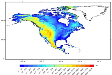
Figure 2. Elevation distribution in North America.

2

3

4

(a)

5

N

1

2

3

. . .

Vegetated area

Vegetated

Glacier

Urban

Lake

Wetland

N

≤

17, up to 17 vegetation patches

Fig. 2. Elevation distribution in North America.

consistency with the PFT map, the elevation raster layer for North America was bilinearly interpolated to 500 m resolu-tion (Fig. 2). We excluded Greenland from our study because HYDRO1k does not cover this area.

2.4 Optimal subgrid classification (SGC) method of elevation and vegetation

The subgrid classification (SGC) method developed in our study considered the joint distribution of elevation and veg-etation. Within each model grid (e.g., at resolution 0.1◦×

0.1◦), the SGC method first classified surface elevation from the 500 m DEM data into a limited number of elevation bands (or classes) of equal elevation range. A minimum area thresh-old of 1 % was used to limit the area of each elevation band. That is, an elevation band containing less than 1 % of the land area of the model grid is added to the neighboring ele-vation band so that each eleele-vation band covers at least 1 % of the grid land area. Within each elevation band in each model grid, the area was further classified into a limited number of PFTs. For example, withMelevation bands within a model grid cell andNPFTs within each elevation band, the model grid was represented with a total number ofM×N subgrid classes or land response units (LRUs), with each elevation– PFT LRU treated as a computational unit in the land sur-face model simulation. The schematic comparison between the new SGC method and CLM subgrid method is shown in Fig. 3.

22 1

Figure 2. Elevation distribution in North America. 2

3

4

(a) 5

N

1

2

3

. . .

Vegetated area

Vegetated Glacier

Urban

Lake

Wetland

N≤17, up to 17 vegetation patches

23 1

(b) 2

Figure 3. Schematic diagram of subgrid classification method in (a) CLM 4.0 and (b) SGC 3

method. 4

5

Figure 4. Baseline subgrid classification method. (a) 0.1°, number of PFTs; (b) 1.0°, number 6

of PFTs; (c) 0.1°, average standard deviation of elevation σ!"; (d) 1.0°, average standard

7

deviation of elevation σ!".

8

N

1

2

3

. . .

PFT classification Vegetated area

Wetland, …

vegetated .  .  .  

Elevation classification

urban, …

vegetated Glacier, …

vegetated

.  .  .  

Fig. 3. Schematic diagram of subgrid classification method in (a)

CLM 4.0 and (b) SGC method.

To restrict computational burden, we set the maximum-allowed total number of LRUs to “N_LRU” (e.g., 18 LRUs) for each model grid. The number of elevation bands M and the number of PFTs N for each elevation band are

Y. Ke et al.: Enhancing the representation of subgrid land surface characteristics 1613

variable for each model grid, butM×N should not exceed the maximum-allowed numberN_LRU (e.g., 18). Hence the combination ofM andN is variable and is chosen to best represent the subgrid variability of both PFT and elevation. For example, for N_LRU=18, possible combinations in-clude 3 elevation bands and 6 PFTs per elevation band, or 2 elevation bands and 9 PFTs per elevation band, etc, but the optimal combination was selected. Two criteria must be sat-isfied for the optimal classification: (1) the elevation range of each elevation band is less than and close to 100 m; and (2) total percentage of subgrid PFTs correctly classified by the method is no less than 80 % for each model grid. We prioritized criteria (2) so that if none of the combinations satisfies both conditions, the classification explaining more than 80 % of PFTs and with elevation range greater than but closest to 100 m was selected; if more than one combination satisfy both conditions, the classification that correctly clas-sifies the most subgrid PFTs was selected.

2.5 SGC method evaluation

In CLM 4.0, vegetation was represented as the composition of 15 PFTs plus bare soil. The simplest and least compu-tationally intensive way to incorporate elevation distribution of vegetation is to assign a single elevation band to each PFT within a model grid; that is, the surface elevation in the area covered by each PFT was aggregated to one elevation band. We used this method as a baseline to assess the performance of the SGC at different model resolutions (0.1◦, 0.25◦, 0.5◦, 1.0◦, and 2.0◦).

The SGC method was also evaluated by comparing it with two other subgrid classification methods based on a fixed number of elevation bands and vegetation types. The first subgrid classification method (SGC1) was theM elevation bands–N PFTs method. Each model grid cell is first divided into M equal-interval elevation bands and each elevation band was further classified intoN PFTs. The second subgrid classification method (SGC2) was theN PFTs–Melevation bands method. Each model grid cell was first classified into N PFTs and the area covered by each PFT was further di-vided intoMequal-interval elevation bands. For both meth-ods, we used the minimum area threshold of 1 % to restrict the number of elevation bands in the same way that was used in the SGC method. The SGC1 and SGC2 methods take dif-ferent perspectives of topography–vegetation distribution in that SGC1 examines the PFT distribution at different eleva-tion bands and SGC2 examines the elevaeleva-tion distribueleva-tion of each PFT. However, both methods classify the model grids into fixed numbers of elevation bands and PFTs throughout the study area.

We implemented the classification methods SGC, SGC1 and SGC2 in North America at 0.1◦, 0.25◦, 0.5◦, 1.0◦ and 2.0◦resolution with different combinations of number of elevation bands and vegetation types: (1) Scheme 1:

N_LRU=24, M=6N=4, meaning 24 maximum-allowed

classes for the SGC method and the combination of 6 eleva-tion bands and 4 PFTs for the SGC1 and SGC2 methods; (2) Scheme 2:N_LRU=18M=6N=3; and (3) Scheme 3: N_LRU=12, M=4N=3. The baseline subgrid method was also implemented at the five resolutions. The three schemes represent different computational burdens with Scheme 1 being most computationally intensive because it has the largest number of maximum-allowed total subgrid LRUs for each model grid.

The average number of total LRUs across NA was used to evaluate and compare the methods’ computational burden. In the baseline method, LRUs correspond to PFTs within each model grid; in the SGC, SGC1 and SGC2 methods, LRUs correspond to elevation–PFT classes within each model grid. The total percentage of PFTs explained within each model grid (% PFT) and the mean standard deviation of elevation averaged over all elevation bandsσepwere used to measure

and compare the methods’ abilities to characterize subgrid vegetation and topography (Eqs. 1–3).

%PFT=

Nb X

i=1



PAeb(i)×

Np X

j=1

PApft(i, j )



, (1)

where PAeb(i)is the percent area of theith elevation band in

that grid, PApft(i,j)is the percent coverage of thejth

domi-nant PFT in theith elevation band,Npis the number of

dom-inant PFTs within each elevation band, andNbis the number

of elevation bands in that grid.

For the SGC and SGC1 methods,σepat a given model grid

was calculated as

σep=

1

Nb

Nb X

i=1

σeb(i), (2)

whereσeb(i)is the standard deviation of subgrid surface

ele-vation within theith elevation band, andNbis the number of

elevation bands in that grid.

For the baseline and SGC2 methods,σepwas calculated as

σep=

1

NP

NP X

j=1

"

1

Nb

Nb X

i=1

σeb(i, j )

#

, (3)

whereσeb(i, j )is the standard deviation of subgrid surface

elevation within theith elevation band for the jth dominant PFT, andNpis the number of dominant PFTs in that grid.

For the baseline method,Np can be any number within 15

because all PFTs within each model grid were included, and Nbequals 1 because only one elevation band was assigned to

each PFT.

3 Results and discussions

3.1 Comparison of the SGC method and the baseline method

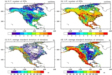
Figure 4 shows the number of PFTs andσepfrom the

base-line subgrid classification method over the NA continent at 0.1◦and 1.0◦resolutions. Both spatial resolutions show simi-lar spatial patterns of subgrid variability of vegetation: more PFT classes (6–8 PFTs at 0.1◦resolution, over 8 PFTs at 1.0◦ resolution) per grid in the coastal areas than in the inland re-gion such as the Great Plains (1–2 PFTs at 0.1◦ resolution, 3–5 PFTs at 1.0◦resolution), where crop dominates the land-scape. Increasing model grid size results in greater subgrid-scale variability of PFTs (Fig. 4a and b). When assigning one elevation band to each PFT within the model grid, the spatial distribution ofσepclearly corresponds with topographic

vari-ations (Fig. 4c and d). In western NA with complex topogra-phy such as the Coastal Range and Rocky Mountains,σepis

larger than in flat areas such as the Great Plains and coastal area in southeast NA. The spatial contrast becomes more dis-tinct at coarser resolution as the subgrid topographic vari-ability becomes larger. The averageσepacross the continent

rapidly increases from 43.1 m at 0.1◦resolution to 62.7 m at 0.25◦resolution, 79.9 m at 0.5◦resolution, 99.1 m at 1.0◦ res-olution, and 123.3 m at 2.0◦resolution, indicating that with the baseline method substantially less subgrid topographic details are represented at coarser resolution.

Figure 5 compares the SGC method and the baseline method in terms of computational burden, % PFT and the elevation variability explained by the methods. Note that although a maximum of 15 PFTs are allowed within each model grid, the computational burden depends on the actual number of PFTs needed to represent the subgrid PFT vari-ability, which can be smaller than 15. It is apparent that SGC is more computationally intensive even withN_LRU (=12) smaller than the maximum number of PFTs in the baseline method (=15). In the baseline method, the average number of PFTs increases from 3.5 to 8.4 at resolutions varying from 0.1 to 2.0 degrees, while the average number of elevation– PFT LRUs in the SGC method increases from 5.5 to 10.6 (N_LRU=12). SGC explained slightly less PFTs than the baseline method that allows all PFTs in each model grid (Fig. 5b). IncreasingN_LRU required more computing re-sources but yielded better PFT representation. However, the small sacrifice in computational burden and % PFT resulted in substantial improvement in elevation variability represen-tation. Figure 5c demonstrates that the standard deviation of elevation within each elevation band is greatly suppressed, with the averageσepof SGC reduced to almost one third that

of the baseline method.

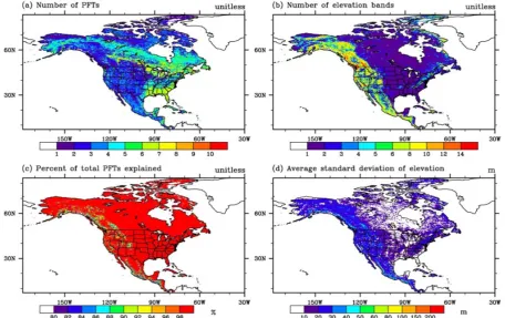
Compared to the baseline method where the number of PFTs and the number of elevation band per PFT (=1) were predetermined, the optimal SGC method produced a much more spatially variant number of elevation bands (M) and

number of PFTs within each elevation band (N )throughout the continent (Figs. 6a, b and 7a, b). In topographically com-plex areas, the SGC method shows great advantage over the baseline method in representing details of subgrid topogra-phy (Fig. 4c vs. Fig. 6d, Fig. 4d vs. Fig. 7d). This advantage is more prominent at coarser resolution as σepis generally

less than 60 m for the SGC method in the Pacific Northwest compared to over 200 m for the baseline method (Fig. 4d vs. Fig. 7d). However, more detailed elevation information in the SGC method compromises the representation of PFTs com-pared to the baseline method that considers all PFTs within each model grid. Nevertheless, the SGC method still ex-plained a reasonable amount of PFT variability (over 80 % in Figs. 6c and 7c, over 94 % in Fig. 5b) while greatly im-proving the elevation variability, which has equally large if not larger impacts on land surface processes than PFT vari-ability (Leung and Ghan, 1998).

3.2 The SGC method with differentN_LRU and model resolutions

The SGC method at different model resolutions (Fig. 6a vs. 7a, Fig. 6b vs. 7b) shows that bothM andN demonstrate a similar spatial pattern in North America. In the areas with more complex topography such as the Coastal Range, Rocky Mountains, and the Appalachian Mountains (Fig. 2), more elevation bands were generated than in flat areas such as the central and coastal plains (Figs. 6b and 7b). The spatial dis-tribution ofNwithin each elevation band, on the other hand, generally shows an opposite pattern (Figs. 6a and 7a) because the combined number of PFTs and elevation bands was re-stricted byN_LRU. In the flat areas of central and eastern NA, more than six PFTs were generated that explained over 98 % of the total PFTs in the model grids. In topographically complex areas such as western NA, although smallerNwere produced than in other areas, the total PFTs explained by the method was still over 80 % for each model grid (Fig. 6c and 7c) because PFT is more correlated with elevation over com-plex terrains. This allows the SGC method to optimally rep-resent subgrid variations in both topography and vegetation. With decreasing model resolutions and increasing num-ber ofN_LRU, the average computational burden increases. At the finest resolution of 0.1◦, the average number of to-tal LRUs increases only slightly with increasing N_LRU (5.6 for N_LRU=12, 6.3 for N_LRU=18, and 6.8 for N_LRU=24)but increases rapidly at resolution of 2◦_(10.7,

14.9, and 18.9 forN_LRU equal 12, 18, and 24) (Fig. 5a). This demonstrates that the low subgrid variability within a small grid cell can be well represented by a small number of subgrid LRUs. As the subgrid topography and vegeta-tion variavegeta-tion increase with coarser model resoluvegeta-tion, more LRUs are required and the method is more restricted by the maximum-allowed number of LRUs. This shows the method’s ability in assigning optimal classes for different model resolutions, and a larger number of maximum-allowed

Y. Ke et al.: Enhancing the representation of subgrid land surface characteristics 1615

23

1

(b)

2

Figure 3. Schematic diagram of subgrid classification method in (a) CLM 4.0 and (b) SGC

3

method.

4

5

Figure 4. Baseline subgrid classification method. (a) 0.1°, number of PFTs; (b) 1.0°, number

6

of PFTs; (c) 0.1°, average standard deviation of elevation

σ

; (d) 1.0°, average standard

7

deviation of elevation

σ

.

8

N

1

2

3

. . .

PFT classification

Vegetated area

Wetland, …

vegetated

.  .  .  

Elevation classification

urban, …

vegetated Glacier, …

vegetated

.  .  .  

Fig. 4. Baseline subgrid classification method. (a) 0.1◦, number of PFTs; (b) 1.0◦, number of PFTs; (c) 0.1◦, average standard deviation of elevationσep; (d) 1.0◦, average standard deviation of elevationσep.

total classes gives more flexibility in assigning the best suit-able combination of elevation bands and PFTs.

3.3 Comparison of three subgrid classification methods

The optimal subgrid classification method, SGC, was evalu-ated against the SGC1 and SGC2 methods with a fixed num-ber of elevation bands and PFTs.

The spatial distribution of the differences in the % PFT (Fig. 8) andσep(Fig. 9) illustrate that at both fine and coarse

resolutions, the SGC method explained less PFTs (nega-tive values of SGC-SGC1 or SGC-SGC2) and produced dis-tinctly lowerσepin the mountainous western NA with

com-plex topography. In these areas, the SGC method required more elevation bands to represent reasonable variations of elevation (e.g., over 6 elevation bands were produced in these areas in Fig. 6b), thus sacrificing the total PFTs repre-sented (only 2–3 PFTs were identified in this area in Fig. 6a compared to four PFTs used in SGC1 and SGC2 methods). In the southeast United States such as Florida, Mississippi, South Carolina and Georgia, and in central Canada, the SGC method identified more PFTs than the other two methods be-cause few elevation classes are needed to represent the flat topography (Fig. 8). Althoughσepin flat areas from SGC is

slightly greater than that from the other two methods (Fig. 9),

SGC is still able to produce reasonable representation of el-evation variability as σep is less than 30 m in these areas

(Figs. 6d and 7d). This implies that using 6 or 4 elevation bands may be redundant in these areas because topography does not vary much and vegetation distribution has little rela-tion to topography. When fewer PFTs were used in SGC1 and SGC2 and fewerN_LRUs were used in SGC, the areas of positive difference in the % PFT between SGC and the other two methods expanded from central Canada to Alberta and Saskatchewan provinces in western Canada (Fig. 8b and e). In Mexico and Central America with distinct topographic re-lief, SGC explained a considerably higher percentage of PFT than SGC2. This emphasizes the advantages of SGC in to-pographically complex and species-rich areas partly because vegetation type correlates with topography.

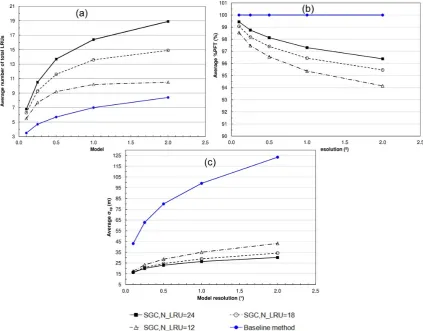
With increasing model grid size and decreasingM orN, the average % PFT represented by each method decreases (Fig. 10a), while the standard deviation of % PFT increases (Fig. 10b). WithM=6, N=4 andN_LRU=24, the SGC1 method, which first classifies topography into 6 elevation bands and represents each elevation band with the 4 most dominant PFTs, explains the most PFTs, while the opti-mal classification method produced the lowest percentage of PFTs except at 0.1◦resolution. With 18 maximum-allowed

Fig. 5. SGC method compared to baseline method. (a) Average number of total LRUs across NA; (b) average %PFT; (c) averageσep.

number of total LRUs in SGC,M=6 andN=3, the neg-ative differences in PFTs between SGC and the other two methods were compensated by positive differences (Fig. 8b and e). Hence overall, the average percentage of PFTs ex-plained by SGC is higher than the other two methods across all resolutions (Fig. 10a). AsN_LRU decreases to 12, at the finest resolution of 0.1◦, SGC explained a slightly greater percentage of PFTs than the other methods. At the resolution of 1◦or higher, SGC explained a lower amount of PFTs than the other two methods. As stated above, at coarse resolution SGC is more restricted by the number of maximum-allowed LRUs because larger variations of PFTs and topography ex-ist. Since topography shows more distinct change than PFTs, the balance between the number of elevation bands and PFTs resulted in less PFTs explained by the method. Although the SGC method shows varying performances in terms of the av-erage percent of PFTs explained compared to the other two methods, the PFTs explained by this method is more spa-tially homogeneous – all model grids in the study area have over 80 % of total PFTs explained regardless ofN_LRU and model resolution. In contrast, the PFTs explained by SGC1 and SGC2 can be as low as 52 % (Fig. 10c), and around

92.7 % of the model grids have over 80 % of the PFTs ex-plained (Fig. 10d).

The abilities of the three methods in explaining topo-graphic variation are shown in Fig. 11. For all three meth-ods, the averageσepincrease with model grid size, i.e.,

re-duced ability to represent subgrid topographic variability as model resolution decreases. At fine resolutions from 0.1◦to 0.5◦, the average σep from the SGC method with N_LRU

of 24 (and 18) is greater than the SGC1 and SGC2 meth-ods withM=6 andN=4 (andN=3)(Fig. 11a), mean-ing that SGC1 and SGC2 have better overall representation of elevation variability at these scales. When model resolu-tion decreases, the advantage of the SGC method in eleva-tion representaeleva-tion emerges. At both 1◦ and 2◦resolutions, the average σep from SGC is lower than that from SGC1

and SGC2. Compared to those from SGC1 and SGC2, the averageσepfrom SGC climbs more slowly with increasing

model grid size and decreasing number of maximum-allowed classes. Because topography shows much greater variability at coarser scales, the slower change in averageσepindicates

more stable performance of the SGC method across different scales. Although the averageσep from SGC is higher than

that from the other methods at fine resolution (e.g., less than

Y. Ke et al.: Enhancing the representation of subgrid land surface characteristics 1617

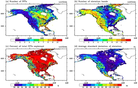
Fig. 6. Optimal classification SGC with maximum-allowed total classesN_class=18 at 0.1◦resolution. (a) number of dominant PFTs classified for each grid; (b) Number of elevation bands classified for each grid; (c) total percentage of PFTs explained by the method;

(d) average standard deviation of elevation in each elevation band in each model gridσep.

1◦), the variation ofσepacross NA is smaller than that from

the other two methods (Fig. 11b) at each model resolution and with each scheme of computational burden. This means that the elevation variability explained by the SGC method is more spatially homogeneous than the other two methods. The combined examination of Figs. 8–11 and the statistical analysis in Table 1 show that the SGC method is not necessar-ily superior to the other two methods in terms of both vegeta-tion and elevavegeta-tion variavegeta-tion explained, when a large number of subgrid classes is allowed (N_LRU=24). However, when computational burden is moderately alleviated using fewer number of subgrid LRUs (N_LRU=18,M=6 andN=3), the SGC method begins to demonstrate its advantage in bal-ancing the variability of vegetation and elevation distribution that can be explained. At the coarser resolutions of 1◦_{to 2}◦_,

the SGC method becomes clearly superior to both SGC1 and SGC2; i.e., a statistically greater percentage of PFTs was ex-plained andσepis smaller (Table 1). WithN_LRU of 12, the

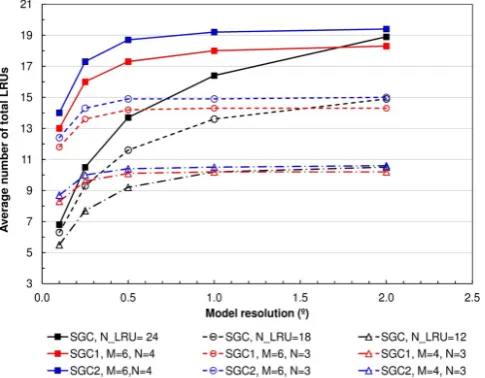
SGC method is better than SGC2 at the resolutions of 0.5◦or coarser and better than SGC1 only at the resolution of 0.25◦. Despite the variable performance of SGC compared to SGC1 and SGC2 in terms of PFT and elevation variabil-ity, SGC is more computationally efficient, especially at fine model resolutions (Fig. 12). For example, in Scheme 1 (N_LRU=24,M=6, N=4), at model resolution of 0.1◦,

the average number of computational units for each model grid for SGC increases quickly from 6.8 to 13.0 and 14.0 for SGC1 and SGC2. With decreasing model resolutions, the differences in computational burden decrease. At coarse res-olution such as 2.0◦, the average number of LRUs are similar for all three methods.

4 Conclusions

In this study we presented a new subgrid land surface repre-sentation method for LSMs that accounts for the joint distri-bution of vegetation and topography. Using updated datasets of high-resolution DEM and PFTs, this study provides a sys-tematic analysis and comparison of different ways to classify subgrid surface elevation and vegetation to provide an opti-mal approach that improves both accuracy and computational efficiency. For each model grid, the new method assigned variable elevation and vegetation classes based on their joint distribution so that the subgrid-scale variability of both can be captured. Using predefinedN_LRU, the method ensures that the optimal combination ofMclasses for elevation and N classes for PFTs is assigned to each model grid under the restriction of a given computational burden. In flat areas with rich vegetation diversity, this method assigns a smallM so

1618 Y. Ke et al.: Enhancing the representation of subgrid land surface characteristics

25

0.1º resolution. (a) number of dominant PFTs classified for each grid; (b) number of elevation

2

bands classified for each grid; (c) Total percentage of PFTs explained by the method; (d)

3

Average standard deviation of elevation in each elevation bands in each model grid σ

.

4

5

Figure 7. Optimal classification SGC with maximum-allowed total classes

!

_

!"#$$

=

18

at

6

1.0º resolution. (a) number of dominant PFTs classified for each grid; (b) number of elevation

7

bands classified for each grid; (c) Total percentage of PFTs explained by the method; (d)

8

Average standard deviation of elevation in each elevation bands in each model grid σ

.

9

10

11

12

13

14

Fig. 7. Optimal classification SGC with maximum-allowed total classesN_class=18 at 1.0◦resolution. (a) Number of dominant PFTs classified for each grid; (b) number of elevation bands classified for each grid; (c) total percentage of PFTs explained by the method;

(d) average standard deviation of elevation in each elevation band in each model gridσep.

Fig. 8. Difference in percentage of total PFTs explained by SGC compared to SGC1 (top row), and SGC compared to SGC2 (bottom row) at

1.0◦model resolution.

Y. Ke et al.: Enhancing the representation of subgrid land surface characteristics 1619

Fig. 9. Difference in average standard deviation of elevation for SGC compared to SGC1 (top row) and SGC compared to SGC2 (bottom

row) at 1.0◦model resolution.

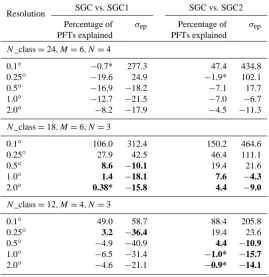
Table 1. Pairedttest statistics for four classification schemes in terms of total PFT explained and standard deviation of elevationσep. Values

in bold indicate significant difference between the two classifications on a 95 % confidence level. Positive value in PFTs and negative value in elevation standard deviation mean better capability of explaining both PFT and elevation. *: not significant.

Resolution SGC vs. SGC1 SGC vs. SGC2 Percentage of σep Percentage of σep

PFTs explained PFTs explained N_class=24, M=6, N=4

0.1◦ −0.7* 277.3 47.4 434.8

0.25◦ −19.6 24.9 −1.9* 102.1 0.5◦ −16.9 −18.2 −7.1 17.7 1.0◦ −12.7 −21.5 −7.0 −6.7 2.0◦ −8.2 −17.9 −4.5 −11.3 N_class=18, M=6, N=3

0.1◦ 106.0 312.4 150.2 464.6

0.25◦ 27.9 42.5 46.4 111.1

0.5◦ 8.6 −10.1 19.4 21.6

1.0◦ 1.4 −18.1 7.6 −4.3

2.0◦ 0.38* −15.8 4.4 −9.0

N_class=12, M=4, N=3

0.1◦ 49.0 58.7 88.4 205.8

0.25◦ 3.2 −36.4 19.4 23.6

0.5◦ −4.9 −40.9 4.4 −10.9

1.0◦ −6.5 −31.4 −1.0* −15.7

2.0◦ −4.6 −21.1 −0.9* −14.1

that a large numberN of PFTs can be represented while el-evation variation is still well represented. However, in topo-graphically complex areas, the method assigns a largerM and a smallerN so that elevation variation can be reason-ably explained. Based on our analysis using high-resolution

DEM and vegetation data, we find that this classification is feasible because, in topographically complex areas, elevation has a dominant influence on vegetation through its effects on climate, so assigning a small number of PFT classes within each elevation class is able to capture the dominant subgrid

Fig. 10. Total PFTs explained by methods SGC, SGC1 and SGC2 across NA. (a) Average % PFT within model grids; (b) standard deviation

of % PFT within model grids; (c) Minimum % PFT within model grids; (d) percentage of grids with total % PFT over 80 %. Black lines: SGC; red lines: SGC1; blue lines: SGC2. Square symbol:N_LRU=24; circular symbol:N_LRU=18; triangular symbol:N_LRU=12.

Fig. 11. Elevation variability explained by methods SGC, SGC1 and SGC2. (a) Averageσep; (b) standard deviation ofσep. Black lines: SGC;

red lines: SGC1; blue lines: SGC2. Square symbol:N_LRU=24; circular symbol:N_LRU=18; triangular symbol:N_LRU=12.

Y. Ke et al.: Enhancing the representation of subgrid land surface characteristics 1621

Fig. 12. Average number of total LRUs of method SGC, SGC1 and

SGC2 across NA. Black lines: SGC; red lines: SGC1; blue lines: SGC2. Square symbol:N_LRU=24; circular symbol:N_LRU= 18; triangular symbol:N_LRU=12.

variations of PFT within the model grid cells. However, we recognized that there is no simple relationship between vege-tation distribution and topography since vegevege-tation cover de-pends not only on elevation but on other environmental fac-tors such as slope/aspect and soil that also play an important role in determining vegetation distribution, so it is important to develop vegetation–elevation distribution for each model grid.

Compared to the baseline method, which assigns a single elevation class to each PFT, the new method provides an ob-vious advantage in representing topographic variability. Al-though the SGC method slightly compromised the ability to represent vegetation variability and increased computational burden compared to the baseline method, the new method still explained at least 80 % of the total PFTs in each model grid and produced substantial improvements in topography representation. The effectiveness of the new method in repre-senting subgrid variability in both topography and vegetation is partly related to the correlation between topography and vegetation. However, this effectiveness decreases with de-creasing model resolution because the elevation dependence of vegetation is weaker at coarser spatial scales.

Compared to the other subgrid approaches with prede-termined number of elevation classes and vegetation types (SGC1 and SGC2), the new method presented in this study balanced the representation of both topography and vegeta-tion variability under the restricvegeta-tion of a maximum-allowed number of total LRUs. With the same maximum-allowed LRUs, it requires less computational burden in LSM simula-tion than the other two methods. Among the three schemes, the new method shows advantages over the other methods with moderate computation intensity (N_LRU=18)and at

coarse scales in that both PFTs and topography variability were best explained. Furthermore, the variability of both veg-etation and elevation explained by the new method was more spatially homogeneous compared to the SGC1 and SGC2 methods regardless of model resolutions and computational burdens.

With the new subgrid scheme, the fractional area of each elevation band and PFT can be determined and the mean elevation of each elevation band can be defined. When im-plemented in the model, each surface elevation class can be forced by different atmospheric conditions by disaggregat-ing the atmospheric forcdisaggregat-ing from each model grid cell to the subgrid elevation class based on temperature and precipita-tion lapse rate or the subgrid parameterizaprecipita-tion of orographic precipitation described in Leung and Ghan (1995, 1998) and Ghan et al. (2006). Separate calculations of surface processes can be performed for each subgrid PFT within each subgrid elevation class, and the output fluxes at each class can be then aggregated in an area-weighted manner for each grid cell. This will allow the impacts of subgrid variations of sur-face topography and PFTs on the partitioning of the energy and water budgets to be represented in land surface models. The impacts of the new subgrid classification on land surface simulations at different model resolutions will be studied in the future.

Acknowledgements. The authors acknowledge the Pacific North-west National Laboratory (PNNL) Integrated Regional Earth System Modeling Initiative, which supported the development of databases used in the study, and the Office of Science of the US Department of Energy through the Earth System Modeling program, which supported the development and analysis of various subgrid classification methods. PNNL is operated by Battelle for the DOE under Contract DE-AC06-76RLO 1830. The authors also acknowledge the support from the Key Program of National Natural Science Foundation of China (NSFC) (41130744/D0107), the General Program of NFSC (41171335/D010702), and the 973 Program of China (2012CB723403).

Edited by: M.-H. Lo

References

Bonan, G. B., Levis, S., Kergoat, L., and Oleson, K. W.: Landscapes as patches of plant functional types: An integrating concept for climate and ecosystem models, Global Biogeochem. Cy., 16, 5-1–5-23, doi:10.1029/2000GB001360, 2002a.

Bonan, G. B., Oleson, K. W., Vertenstein, M., Levis, S., Zeng, X., Dai, Y., Dickinson, R. E., and Yang, Z. L.: The land surface cli-matology of the Community Land Model coupled to the NCAR Community Climate Model, J. Climate, 15, 3123–3149, 2002b. Ek, M. B., Mitchell, K. E., Lin, Y., Rogers, E., Grunmann, P.,

Ko-ren, V., Gayno, G., and Tarpley, J. D.: Implementation of Noah land surface model advances in the National Centers for Environ-mental Prediction operational mesoscale Eta model, J. Geophys. Res., 108, D228851, doi:10.1029/2002JD003296, 2003.

Ghan, S. J., Liljegren, J. C., Shaw, W. J., Hubbe, J. H., and Doran, J. C.: Influence of subgrid variability on surface hydrology, J. Climate, 10, 3157–3166, 1997.

Ghan, S. J., Shippert, T. R., and Fox, J.: Physically based global downscaling: regional evaluation, J. Climate, 19, 429–445, doi:10.1175/JCLI3622.1, 2006.

Giorgi, F. and Avissar, R.: Representation of heterogeneity effects in earth system modeling: Experience from land surface modeling, Rev. Geophys., 35, 413–437, doi:10.1029/97RG01754, 1997. Giorgi, F., Francisco, R., and Pal, J.: Effects of a subgrid-scale

topography and land use scheme on the simulation of sur-face climate and hydrology, Part I: Effects of temperature and water vapor disaggregation, J. Hydrometerol., 4, 317–333, doi:10.1175/1525-7541(2003)4<317:EOASTA>2.0.CO;2, 2003. Hijmans, R. J., Cameron, S. E., Parra, J. L., Jones, P. G., and Jarvis, A.: Very high resolution interpolated climate sur-faces for global land areas, Int. J. Climatol., 25, 1965–1978, doi:10.1002/joc.1276, 2005.

Ke, Y., Leung, L. R., Huang, M., Coleman, A. M., Li, H., and Wig-mosta, M. S.: Development of high resolution land surface pa-rameters for the Community Land Model, Geosci. Model Dev., 5, 1341–1362, doi:10.5194/gmd-5-1341-2012, 2012.

Koster, R. D. and Suarez, M. J.: A comparative analysis of two land surface heterogeneity representations, J. Climate, 5, 1379–1390, doi:10.1175/1520-0442(1992)005<1379:ACAOTL>2.0.CO;2, 1992.

Krinner, G., Viovy, N., de Noblet-Ducoudré, N., Ogée, J., Polcher, J., Friedlingstein, P., Ciais, P., Sitch, S., and Prentice, I. C.: A dynamic global vegetation model for studies of the cou-pled atmosphere-biosphere system, Global Biogeochem. Cy., 19, GB1015, doi:10.1029/2003GB002199, 2005.

Krinner, G., Lezine, A.-M., Braconnot, P., Sepulchre, P., Ram-stein, G., Grenier, C., and Gouttevin, I.: A reassessment of lake and wetland feedbacks on the North African Holocene climate, Geophys. Res. Lett., 39, L07701, doi:10.1029/2012GL0500992, 2012.

Lawrence, D., Oleson, K. W., Flanner, M. G., Thorton, P. E., Swenson, S. C., Lawrence, P. J., Zeng, X., Yang, Z. L., Levis, S., and Skaguchi, K.: Parameterization improvements and func-tional and structural advances in version 4 of the Commu-nity Land Model, J. Adv. Model. Earth Syst., 3, M03001, doi:10.1029/2011MS000045, 2011.

Lawrence, P. J. and Chase, T. N.: Representing a new MODIS con-sistent land surface in the Community Land Model (CLM 3.0), J. Geophys. Res., 112, G01023, doi:10.1029/2006JG000168, 2007. Leung, L. R. and Ghan, S. J.: A subgrid parameterization of orographic precipitation, Theor. App. Climatol., 52, 95–118, doi:10.1007/BF00865510, 1995.

Leung, L. R. and Ghan, S. J.: Parameterizing subgrid oro-graphic precipitation and surface cover in climate mod-els, Mon. Weather Rev., 126, 3271–3291, doi:10.1175/1520-0493(1998)126<3271:PSOPAS>2.0.CO;2, 1998.

Li, H., Wigmosta, M. S., Wu, H., Huang, M., Ke, Y., Coleman, A. M. and Leung, L. R.: A physically based runoff routing model for land surface and earth system models, J. Hydromet., 14, 808– 828, doi:10.1175/JHM-D-12-015.1, 2013.

Li, R. and Arora, V. K.: Effect of mosaic representation of vegeta-tion in land surface schemes on simulated energy and carbon bal-ances, Biogeosciences, 9, 593–605, doi:10.5194/bg-9-593-2012, 2012.

Liang, X., Lettenmaier, D. P., Wood, E. F., and Burges, S. J.: A simple hydrologically based model of land surface water and en-ergy fluxes for general circulation models, J. Geophys. Res., 99, 14415–14428, 1994.

Nijssen, B., Schnur, R., and Lettenmaier, D. P.: Global retrospective estimation of soil moisture using the variable infiltration capac-ity land surface model, 1980–93, J. Climate, 14, 1790–1808, doi:10.1175/1520-0442(2001)014<1790:GREOSM>2.0.CO;2, 2001.

Niu, G.-Y., Yang, Z.-L., Mitchell, K. E., Chen, F., Ek, M. B., Barlage, M., Kumar, A., Manning, K., Niyogi, D., Rosero, E., Tewari, M., and Xia, Y.: The community Noah land surface model with multiparameterization options (Noah©MP): 1.Model description and evaluation with local-scale measurements, J. Geophys. Res., 116, D12109, doi:10.1029/2010JD015139, 2011. Oleson, K. W. and Bonan, G. B.: The effects of remotely sensed plant functional type and leaf area index on simula-tions of boreal forest surface fluxes by the NCAR land sur-face model, J. Hydrometeorol., 1, 431–446, doi:10.1175/1525-7541(2000)001<0431:TEORSP>2.0.CO;2, 2000.

Oleson, K. W., Lawrence, D. M., Bonan, G. B., Flanner, M. G., Kluzek, E., Lawrence, P. J., Levis, S., Swenson, S. C., Thornton, P. E., Dai, A., Decker, M., Dickinson, R., Feddema, J., Heald, C.L., Hoffman, F., Lamarque, J.-F., Mahowald, N., Niu, G.-Y., Qian, T., Randerson, J., Running, S., Sakaguchi, K., Slater, A., Stockli, R., Wang, A., Yang, Z.-L., Zeng, X., and Zeng, X.: Technical Description of version 4.0 of the Community Land Model (CLM). National Center for Atmospheric Research, Boul-der, CO, NCAR/TN-478+STR, 2010.

Seth, A., Giorgi, F., and Dickinson, R. E.: Simulating fluxes from heterogeneous land surfaces: Explicit subgrid method employing the biosphere-atmosphere transfer scheme (BATS), J. Geophys. Res., 99, 18651–18667, doi:10.1029/94JD01330, 1994. Sitch, S., Smith, B., Prentice, I. C., Arneth, A., Bondeau, A.,

Cramer, W., Kaplan, J. O., Levis, S., Lucht, W., Sykes, M. T., Thonicke, K., and Kenevsky, S.: Evaluation of ecosystem dy-namics, plant geography and terrestrial carbon cycling in the LPJ dynamic global vegetation model, Global. Change Biol., 9, 161– 185, 2003.

Still, C., Berry, J. C., Collatz, G. J., and DeFries, R. S.: Global distribution of C3 and C4 vegetation: carbon cy-cle implications, Global Biogeochem. Cy., 17, 6-1–6-14, doi:10.1029/2001GB001807, 2003.