Motivation Discounting Discounting Plant-Level Optimization Results
Do Interest Rates Smooth Investment?
Russell Cooper1 Jon Willis2 1Pennsylvania State University 2Federal Reserve Bank of Kansas City
Motivation Discounting Discounting Plant-Level Optimization Results
Question: How do variations in the interest rate influence
plant-level and aggregate investment?
The answer will improve our understanding of:
Motivation Discounting Discounting Plant-Level Optimization Results
Micro evidence
Investment at the plant level is characterized by infrequent adjustment.
Motivation Discounting Discounting Plant-Level Optimization Results
Micro evidence
Investment at the plant level is characterized by infrequent adjustment.
Motivation Discounting Discounting Plant-Level Optimization Results
Previous research
Research of Thomas (2002), Khan and Thomas (2003), and Khan and Thomas (2008) concludes that non-convexities at the plant level are not important for aggregate investment.
State dependent interest rates in these models are determined in equilibrium.
The striking result is the absence of aggregate effects of lumpy investment.
Motivation Discounting Discounting Plant-Level Optimization Results
Previous research
Research of Thomas (2002), Khan and Thomas (2003), and Khan and Thomas (2008) concludes that non-convexities at the plant level are not important for aggregate investment. State dependent interest rates in these models are determined in equilibrium.
The striking result is the absence of aggregate effects of lumpy investment.
Motivation Discounting Discounting Plant-Level Optimization Results
Our focus
In studying the investment decisions of establishments, what interest rate process are they responding to?
Our focus is studying the effects of interest rate movements found in the data.
Motivation Discounting Discounting Plant-Level Optimization Results
Our focus
In studying the investment decisions of establishments, what interest rate process are they responding to?
Our focus is studying the effects of interest rate movements found in the data.
Motivation Discounting Discounting Plant-Level Optimization Results
Our focus
In studying the investment decisions of establishments, what interest rate process are they responding to?
Our focus is studying the effects of interest rate movements found in the data.
Motivation Discounting Discounting Plant-Level Optimization Results
Key theme: Specifying an interest rate process
Why distinguish data-based interest rate process from model-based interest rate process?
Table: Interest rate properties
Std. dev. relative Correlation to output with output
Data .444 -.385
Benchmark (RBC) .096 .889
State-dependent adjustment .095 .892
Motivation Discounting Discounting Plant-Level Optimization Results
Roadmap for presentation
1 Model with non-convex adjustment costs for investment 2 Specify interest rate process (state dependent discount factor) 3 Specify aggregate process: detrending specification has strong
Motivation Discounting Discounting Plant-Level Optimization Results
Results
Plant-level moments used to estimate parameters in PE studies are insensitive to interest rate process
Specification of interest rate process strongly influences plant-level and aggregate investment response to shocks Specification of aggregate shock process strongly influences the responsiveness of investment to aggregate shock Observed extensive margin of investment behavior supports data-based interest rate process
Motivation Discounting Discounting Plant-Level Optimization Results
Results
Plant-level moments used to estimate parameters in PE studies are insensitive to interest rate process
Specification of interest rate process strongly influences plant-level and aggregate investment response to shocks
Specification of aggregate shock process strongly influences the responsiveness of investment to aggregate shock Observed extensive margin of investment behavior supports data-based interest rate process
Motivation Discounting Discounting Plant-Level Optimization Results
Results
Plant-level moments used to estimate parameters in PE studies are insensitive to interest rate process
Specification of interest rate process strongly influences plant-level and aggregate investment response to shocks Specification of aggregate shock process strongly influences the responsiveness of investment to aggregate shock
Observed extensive margin of investment behavior supports data-based interest rate process
Motivation Discounting Discounting Plant-Level Optimization Results
Results
Plant-level moments used to estimate parameters in PE studies are insensitive to interest rate process
Specification of interest rate process strongly influences plant-level and aggregate investment response to shocks Specification of aggregate shock process strongly influences the responsiveness of investment to aggregate shock Observed extensive margin of investment behavior supports data-based interest rate process
Motivation Discounting Discounting Plant-Level Optimization Results
Results
Plant-level moments used to estimate parameters in PE studies are insensitive to interest rate process
Specification of interest rate process strongly influences plant-level and aggregate investment response to shocks Specification of aggregate shock process strongly influences the responsiveness of investment to aggregate shock Observed extensive margin of investment behavior supports data-based interest rate process
Motivation Discounting Discounting Plant-Level Optimization Results
Our Approach
1 Decentralized solution for establishment’s problem with empirically consistent
State dependent discounting
Adjustment costs for investment
Heterogeneity in productivity
Monopolistic competition
Use equilibrium prices instead of planner’s problem
2 To study:
Smoothing effects of state-dependent discounting
Effects of variation in the interest rate on plant-level and
Motivation Discounting Discounting Plant-Level Optimization Results
State-Dependent Discount Factor (SDDF)
Household optimization for any asset j: Et h
˜
βt+1Rtj+1
i
= 1
Asset pricing kernel: ˜βt+1= βU
0(C t+1)
U0(C t)
Establishment-level problem (stationary):
V(A, ε,k,Z) = max
k0
π(A, ε,k)−C(A, ε,k,k0) +
EA0,Z0,ε0|A,Z,ε[ ˜β(·)V(A0, ε0,k0,Z0)] o
Monetary Policy targets RtM+1 conditional onZt andZt+1
Impacts Euler Equation
Motivation Discounting Discounting Plant-Level Optimization Results
State-Dependent Discount Factor (SDDF)
Household optimization for any asset j: Et h
˜
βt+1Rtj+1
i
= 1 Asset pricing kernel: ˜βt+1= βU
0(C t+1)
U0(C t)
Establishment-level problem (stationary):
V(A, ε,k,Z) = max
k0
π(A, ε,k)−C(A, ε,k,k0) +
EA0,Z0,ε0|A,Z,ε[ ˜β(·)V(A0, ε0,k0,Z0)] o
Monetary Policy targets RtM+1 conditional onZt andZt+1
Impacts Euler Equation
Motivation Discounting Discounting Plant-Level Optimization Results
Issues
Asset Pricing
Can we rely on the HH Euler equation to price assets, including investment and the federal funds market?
Canzoneri et al. (2007) find huge differences between money market rates and (parameterized) HH Euler equations. Is this the right channel for monetary policy?
What are the adjustment costs at the plant-level?
Cooper and Haltiwanger (2006)
Includes market power and heterogeneity
Check moment implications with state dependent discounting
Motivation Discounting Discounting Plant-Level Optimization Results
Issues
Asset Pricing
Can we rely on the HH Euler equation to price assets, including investment and the federal funds market?
Canzoneri et al. (2007) find huge differences between money market rates and (parameterized) HH Euler equations.
Is this the right channel for monetary policy?
What are the adjustment costs at the plant-level?
Cooper and Haltiwanger (2006)
Includes market power and heterogeneity
Check moment implications with state dependent discounting
Motivation Discounting Discounting Plant-Level Optimization Results
Issues
Asset Pricing
Can we rely on the HH Euler equation to price assets, including investment and the federal funds market?
Canzoneri et al. (2007) find huge differences between money market rates and (parameterized) HH Euler equations. Is this the right channel for monetary policy?
What are the adjustment costs at the plant-level?
Cooper and Haltiwanger (2006)
Includes market power and heterogeneity
Check moment implications with state dependent discounting
Motivation Discounting Discounting Plant-Level Optimization Results
Issues
Asset Pricing
Can we rely on the HH Euler equation to price assets, including investment and the federal funds market?
Canzoneri et al. (2007) find huge differences between money market rates and (parameterized) HH Euler equations. Is this the right channel for monetary policy?
What are the adjustment costs at the plant-level?
Cooper and Haltiwanger (2006)
Includes market power and heterogeneity
Check moment implications with state dependent discounting
Motivation Discounting Discounting Plant-Level Optimization Results
What interest rate should be used to discount plant level profits?
1 Model Based:
Interest rate derived from general equilibrium model (Thomas
(2002), Khan and Thomas (2003), and others)
Mapping from states to interest rates determined within model
2 Data Based:
Estimate functional relationship between Euler-equation-based
discount rate and aggregate state variables
Coefficients from data not model
3 Estimate state-dependent market rates directly
Motivation Discounting Discounting Plant-Level Optimization Results
Finding the pricing kernel: ˜
β
=
B
(
·
)
Use the Data
1 Calculate ˜βt+1=βU
0(C t+1) U0(C
t) from data
2 SpecifyB(·)
3 Estimate it from aggregate data
Use a Model
1 Stochastic Growth Model with Monopolistic Competition (eg.
Chatterjee and Cooper (1993))
2 Ct=C(At,Kt),Kt+1=K(At,Kt) , ˜βt+1= βU
0(C t+1) U0(Ct)
3 (A,K) are aggregate state variables
4 Solve model and obtain evolution of states and controls to
Motivation Discounting Discounting Plant-Level Optimization Results
Estimating
B
(
A
t,
A
t+1,
K
t)
Data: follow Stock and Watson (1999)
Consumption = Nondurables + Services (BEA)
Output = Real Business Nonfarm GDP (BEA)
Labor = Private nonfarm payroll employment (BLS)
Capital = Real private nonresidential fixed capital stock (BEA)
log(A) = log(Output) - 0.65*log(Labor) - 0.35*log(Capital)
Details:
Annual data from 1948 - 2008
Motivation Discounting Discounting Plant-Level Optimization Results
Estimating
B
(
A
t,
A
t+1,
K
t)
1 Construct ˜βt+1= βU
0(C t+1)
U0(C
t) using U(C) =log(C) and β = 0.96
2 Regress ˜βt+1 on{At,At+1,Kt}
Motivation Discounting Discounting Plant-Level Optimization Results
Side Note: Filtering the data
1940 1950 1960 1970 1980 1990 2000 2010
−1 −0.9 −0.8 −0.7 −0.6 −0.5 −0.4 −0.3 −0.2 −0.1 0 Solow residual log level
1940 1950 1960 1970 1980 1990 2000 2010
−0.1 −0.08 −0.06 −0.04 −0.02 0 0.02 0.04 0.06 0.08 0.1
Filtered Solow residual
log deviation from trend
! = 0.84
Motivation Discounting Discounting Plant-Level Optimization Results
Side Note: Filtering the data
−11940 1950 1960 1970 1980 1990 2000 2010−0.9 −0.8 −0.7 −0.6 −0.5 −0.4 −0.3 −0.2 −0.1 0 Solow residual log level
1940 1950 1960 1970 1980 1990 2000 2010
−0.1 −0.08 −0.06 −0.04 −0.02 0 0.02 0.04 0.06 0.08 0.1
Filtered Solow residual
log deviation from trend
! = 0.84
Motivation Discounting Discounting Plant-Level Optimization Results
Side Note: Filtering the data
1940 1950 1960 1970 1980 1990 2000 2010
−0.1 −0.08 −0.06 −0.04 −0.02 0 0.02 0.04 0.06 0.08 0.1
Filtered Solow residuals
log deviation from trend
! = 0.84
! = 0.14
Linear filter ("=100000) Band Pass filter (" = 7)
1940 1950 1960 1970 1980 1990 2000 2010
−0.15 −0.1 −0.05 0 0.05 0.1 0.15
Filtered Solow residual
log deviation from trend
Motivation Discounting Discounting Plant-Level Optimization Results
Pricing kernel (SDDF): ˜
β
=
B
(
A
t,
A
t+1,
K
t)
Source At At+1 Kt R2 dEtdA[ ˜βt(·)]
Case 1 Data 0.34 -0.46 0.01 0.56 -0.04
λ= 100000 (0.05) (0.06) (0.03)
(ρA = 0.84) Chat-Coop 0.43 -0.64 0.09 NA -0.11
KPR 0.37 -0.59 0.09 NA -0.12
Motivation Discounting Discounting Plant-Level Optimization Results
Pricing kernel (SDDF): ˜
β
=
B
(
A
t,
A
t+1,
K
t)
Source At At+1 Kt R2 dEtdA[ ˜βt(·)]
Case 1 Data 0.34 -0.46 0.01 0.56 -0.04
λ= 100000 (0.05) (0.06) (0.03)
(ρA = 0.84) Chat-Coop 0.43 -0.64 0.09 NA -0.11
KPR 0.37 -0.59 0.09 NA -0.12
Motivation Discounting Discounting Plant-Level Optimization Results
Pricing kernel (SDDF): ˜
β
=
B
(
A
t,
A
t+1,
K
t)
Source At At+1 Kt R2 dEtdA[ ˜βt(·)]
Case 1 Data 0.34 -0.46 0.01 0.56 -0.04
λ= 100000 (0.05) (0.06) (0.03)
(ρA = 0.84) Chat-Coop 0.43 -0.64 0.09 NA -0.11
KPR 0.37 -0.59 0.09 NA -0.12
Motivation Discounting Discounting Plant-Level Optimization Results
Pricing kernel (SDDF): ˜
β
=
B
(
A
t,
A
t+1,
K
t)
Source At At+1 Kt R2 dEtdA[ ˜βt(·)]
Case 1 Data 0.34 -0.46 0.01 0.56 -0.04
λ= 100000 (0.05) (0.06) (0.03)
(ρA = 0.84) Chat-Coop 0.43 -0.64 0.09 NA -0.11
KPR 0.37 -0.59 0.09 NA -0.12
Motivation Discounting Discounting Plant-Level Optimization Results
Pricing kernel (SDDF): ˜
β
=
B
(
A
t,
A
t+1,
K
t)
Source At At+1 Kt R2 dEtdA[ ˜βt(·)]
Case 3 Data 0.20 -0.59 0.06 0.46 0.12
λ= 7 (0.09) (0.10) (0.15)
(ρA = 0.14) Chat-Coop 0.09 -0.41 0.09 NA 0.03
KPR 0.08 -0.39 0.09 NA 0.03
Motivation Discounting Discounting Plant-Level Optimization Results
Pricing kernel (SDDF): ˜
β
=
B
(
A
t,
A
t+1,
K
t)
Source At At+1 Kt R2 dEtdA[ ˜βt(·)]
Case 3 Data 0.20 -0.59 0.06 0.46 0.12
λ= 7 (0.09) (0.10) (0.15)
(ρA = 0.14) Chat-Coop 0.09 -0.41 0.09 NA 0.03
KPR 0.08 -0.39 0.09 NA 0.03
Motivation Discounting Discounting Plant-Level Optimization Results
State-Dependent Discount Factor (SDDF)
−40 5 10 15 20 25 30 35 40 45 50 −20 2 4
Aggregate shock and expected discount factor (E[!]) when "A = 0.14
periods (years)
percentage log deviation from steady state
0 5 10 15 20 25 30 35 40 45 50−0.4
−0.2 0 0.2 0.4
percentage log deviation from steady state
Aggregate profitability shock (left axis) Empirical discount factor (right axis) Chat−Coop discount factor (right axis)
0 5 10 15 20 25 30 35 40 45 50
−6 −4 −2 0 2 4 6
Aggregate shock and expected discount factor (E[!]) when "A = 0.84
periods (years)
percentage log deviation from steady state
0 5 10 15 20 25 30 35 40 45 50−0.6
−0.4 −0.2 0 0.2 0.4 0.6
percentage log deviation from steady state
Motivation Discounting Discounting Plant-Level Optimization Results
Stochastic Discount Factor
0 5 10 15 20 25 30 35 40 45 50
−4
−2 0 2 4
Aggregate shock and expected discount factor (E[!]) when "A = 0.14
periods (years)
percentage log deviation from steady state
0 5 10 15 20 25 30 35 40 45 50−0.4
−0.2 0 0.2 0.4
percentage log deviation from steady state
Aggregate profitability shock (left axis) Empirical discount factor (right axis) Chat−Coop discount factor (right axis)
0 5 10 15 20 25 30 35 40 45 50
−6 −4 −2 0 2 4 6
Aggregate shock and expected discount factor (E[!]) when "A = 0.84
periods (years)
percentage log deviation from steady state
0 5 10 15 20 25 30 35 40 45 50−0.6
−0.4 −0.2 0 0.2 0.4 0.6
percentage log deviation from steady state
Motivation Discounting Discounting Plant-Level Optimization Results
Experiments
Questions
1 What are the effects of interest rates on aggregate and plant-level investment?
2 Is there smoothing of nonconvexities through state-dependent discounting?
Study by comparing outcomes
Motivation Discounting Discounting Plant-Level Optimization Results
Experiments
Questions
1 What are the effects of interest rates on aggregate and plant-level investment?
2 Is there smoothing of nonconvexities through state-dependent discounting?
Study by comparing outcomes
Motivation Discounting Discounting Plant-Level Optimization Results
Plant-Level Optimization Problem
V(A, ,k) = max{Vi(A, ε,k),Va(A, ε,k)}, ∀(A, ε,k),
where
Vi(A, ε,k) = Π(A, ε,k) +EA0,ε0|A,ε
h
˜
βV(A0, ε0,k(1−δ))i
Va(A, ε,k) = max
k0 Π(A, ε
0,k)−C(A, ε,k,k0) +
EA0,ε0|A,ε
h
˜
βV(A0, ε0,k0)i
where
C(A, ε,k,k0) =
disruption cost
z }| {
(1−λ) Π(A, ε0,k) +pb(I>0)(k0−(1−δ)k)
−ps(I<0)((1−δ)k−k0)
| {z }
irreversibility
+ν 2
k0−(1−δ)k k
2 k
| {z }
Motivation Discounting Discounting Plant-Level Optimization Results
Cooper and Haltiwanger (2006)
Three forms of investment adjustment costs:
disruption cost (λ)
quadratic adjustment cost (ν)
irreversibility (ps)
Estimate {λ, ν,ps} via SMM
Motivation Discounting Discounting Plant-Level Optimization Results
Parameters:
From CH (2006)
λ= 0.8
ν = 0.15
ps =0.98 ρε = 0.88
σε = 0.1
Constant returns to scale
θ = 5
Motivation Discounting Discounting Plant-Level Optimization Results
State Dependent Discounting and Plant-Level Investment
Plant-level moments used in CH (2006) estimation are insensitive to ˜β
Table: Plant-level moments
Model Corr(i,i−1) Corr(i, ε) Spike + Spike
-β -0.13 0.19 0.13 0
˜
Motivation Discounting Discounting Plant-Level Optimization Results
Plant-level investment regression on simulated data:
I
i(
A
, ε
i,
K
i)
Model ρA A εi Ki R2
β 0.14 -12.78 28.47 -0.46 0.36
(3.22) (0.26) (0.00)
0.84 23.59 29.82 -0.43 0.36
(1.37) (0.27) (0.00)
˜
β(At,At+1) 0.14 24.58 28.40 -0.46 0.36
(Empirical) (3.22) (0.26) (0.00)
0.84 13.76 29.74 -0.43 0.36
(1.37) (0.27) (0.00)
˜
β(At,At+1) 0.14 -1.97 28.63 -0.46 0.36
(Chat-Coop) (3.21) (0.26) (0.00)
0.84 -6.48 30.20 -0.44 0.36
Motivation Discounting Discounting Plant-Level Optimization Results
Intensive margin
Table:Plant-level investment regression (Adjusters only):Ii(A, εi,Ki)
Model ρA A εi Ki R2
β 0.14 4.54 25.54 0.02 0.90
(2.57) (0.45) (0.01)
0.84 26.11 29.58 0.02 0.98
(0.56) (0.23) (0.01) ˜
β(At,At+1) 0.14 17.11 24.60 0.04 0.90
(Empirical) (2.59) (0.45) (0.01)
0.84 18.42 29.61 0.03 0.98
(0.50) (0.21) (0.00) ˜
β(At,At+1) 0.14 5.28 25.25 0.03 0.90
(Chat-Coop) (2.51) (0.44) (0.01)
0.84 2.80 29.67 0.03 0.99
Motivation Discounting Discounting Plant-Level Optimization Results
Extensive margin
Table:Linear probability regression using plant-level simulated data (extensive
margin)
Model ρA A εi Ki R2
β 0.14 -0.67 1.25 -0.84 0.37
(0.15) (0.01) (0.01)
0.84 1.00 1.26 -0.81 0.37
(0.06) (0.01) (0.01) ˜
β(At,At+1) 0.14 1.17 1.25 -0.84 0.37
(Empirical) (0.15) (0.01) (0.01)
0.84 0.58 1.24 -0.79 0.37
(0.06) (0.01) (0.01) ˜
β(At,At+1) 0.14 -0.11 1.26 -0.85 0.37
(Chat-Coop) (0.15) (0.01) (0.01)
0.84 -0.33 1.27 -0.81 0.37
Motivation Discounting Discounting Plant-Level Optimization Results
Aggregate Investment
0 5 10 15 20 25 30
−0.03 −0.02 −0.01 0 0.01 0.02 0.03 0.04 periods (years)
deviation from mean
Aggregate shock and aggregate investment rate (I/K) when !A = 0.14
0 5 10 15 20 25 30−0.03
−0.02 −0.01 0 0.01 0.02 0.03 0.04
deviation from mean
Aggregate profitability shock (left axis) Investment rate (fixed ") (right axis)
0 5 10 15 20 25 30
−0.06 −0.03 0 0.03 0.06 0.09
Aggregate shock and aggregate investment rate (I/K) when !A = 0.84
periods (years)
deviation from mean
0 5 10 15 20 25 30−0.04
−0.02 0 0.02 0.04 0.06
deviation from mean
Motivation Discounting Discounting Plant-Level Optimization Results
Aggregate Investment
0 5 10 15 20 25 30
−0.03 −0.02 −0.01 0 0.01 0.02 0.03 0.04 periods (years)
deviation from mean
Aggregate shock and aggregate investment rate (I/K) when !A = 0.14
0 5 10 15 20 25 30−0.03
−0.02 −0.01 0 0.01 0.02 0.03 0.04
deviation from mean
Aggregate profitability shock (left axis)
Investment rate (fixed ") (right axis)
Investment (empirical) (right axis)
0 5 10 15 20 25 30
−0.06 −0.03 0 0.03 0.06 0.09
Aggregate shock and aggregate investment rate (I/K) when !A = 0.84
periods (years)
deviation from mean
0 5 10 15 20 25 30−0.04
−0.02 0 0.02 0.04 0.06
deviation from mean
Aggregate profitability shock (left axis)
Investment rate (fixed ") (right axis)
Motivation Discounting Discounting Plant-Level Optimization Results
Aggregate Investment
0 5 10 15 20 25 30
−0.03 −0.02 −0.01 0 0.01 0.02 0.03 0.04 periods (years)
deviation from mean
Aggregate shock and aggregate investment rate (I/K) when !A = 0.14
0 5 10 15 20 25 30−0.03
−0.02 −0.01 0 0.01 0.02 0.03 0.04
deviation from mean
Aggregate profitability shock (left axis)
Investment rate (fixed ") (right axis)
Investment (empirical) (right axis)
Investment (Chat−Coop) (right axis)
0 5 10 15 20 25 30
−0.06 −0.03 0 0.03 0.06 0.09
Aggregate shock and aggregate investment rate (I/K) when !A = 0.84
periods (years)
deviation from mean
0 5 10 15 20 25 30−0.04
−0.02
0 0.02 0.04 0.06
deviation from mean
Aggregate profitability shock (left axis)
Investment rate (fixed ") (right axis)
Investment (empirical) (right axis)
Motivation Discounting Discounting Plant-Level Optimization Results
Aggregate Investment
0 5 10 15 20 25 30
−0.03 −0.02 −0.01 0 0.01 0.02 0.03 0.04 periods (years)
deviation from mean
Aggregate shock and aggregate investment rate (I/K) when !A = 0.14
0 5 10 15 20 25 30−0.03
−0.02 −0.01 0 0.01 0.02 0.03 0.04
deviation from mean
Aggregate profitability shock (left axis) Investment rate (fixed ") (right axis)
0 5 10 15 20 25 30
−0.06 −0.03 0 0.03 0.06 0.09
Aggregate shock and aggregate investment rate (I/K) when !A = 0.84
periods (years)
deviation from mean
0 5 10 15 20 25 30−0.04
−0.02
0 0.02 0.04 0.06
deviation from mean
Motivation Discounting Discounting Plant-Level Optimization Results
Aggregate Investment
0 5 10 15 20 25 30
−0.03 −0.02 −0.01 0 0.01 0.02 0.03 0.04 periods (years)
deviation from mean
Aggregate shock and aggregate investment rate (I/K) when !A = 0.14
0 5 10 15 20 25 30−0.03
−0.02 −0.01 0 0.01 0.02 0.03 0.04
deviation from mean
Aggregate profitability shock (left axis) Investment rate (fixed ") (right axis) Investment (empirical) (right axis)
0 5 10 15 20 25 30
−0.06 −0.03 0 0.03 0.06 0.09
Aggregate shock and aggregate investment rate (I/K) when !A = 0.84
periods (years)
deviation from mean
0 5 10 15 20 25 30−0.04
−0.02 0 0.02 0.04 0.06
deviation from mean
Motivation Discounting Discounting Plant-Level Optimization Results
Aggregate Investment
0 5 10 15 20 25 30
−0.03 −0.02 −0.01 0 0.01 0.02 0.03 0.04 periods (years)
deviation from mean
Aggregate shock and aggregate investment rate (I/K) when !A = 0.14
0 5 10 15 20 25 30−0.03
−0.02 −0.01 0 0.01 0.02 0.03 0.04
deviation from mean
Aggregate profitability shock (left axis)
Investment rate (fixed ") (right axis)
Investment (empirical) (right axis)
Investment (Chat−Coop) (right axis)
0 5 10 15 20 25 30
−0.06 −0.03 0 0.03 0.06 0.09
Aggregate shock and aggregate investment rate (I/K) when !A = 0.84
periods (years)
deviation from mean
0 5 10 15 20 25 30−0.04
−0.02 0 0.02 0.04 0.06
deviation from mean
Aggregate profitability shock (left axis)
Investment rate (fixed ") (right axis)
Investment (empirical) (right axis)
Motivation Discounting Discounting Plant-Level Optimization Results
Correlation of aggregates with aggregate shock (A)
Extensive Margin Intensive Margin
Model ρA I K KI Fraction of adjusters mean(Ii Ki|
Ii Ki>0.2)
Data 0.14 0.08 -0.02 0.12 0.14 NA
0.84 0.05 -0.36 0.23 0.19 NA
β 0.14 -0.51 0.03 -0.50 -0.55 0.61
0.84 0.55 0.73 0.43 0.46 0.09
˜
β(At,At+1) 0.14 0.61 0.15 0.58 0.62 0.01
(Empirical) 0.84 0.47 0.69 0.36 0.36 0.47
˜
β(At,At+1) 0.14 -0.19 0.10 -0.20 -0.23 0.49
Motivation Discounting Discounting Plant-Level Optimization Results
Extensive margin
0 5 10 15 20 25 30 35 40 45 50
−0.04
−0.02 0 0.02 0.04
Extensive margin when ρA = 0.14
periods (years)
profitability shock
0 5 10 15 20 25 30 35 40 45 500.08
0.1 0.12 0.14 0.16
fraction of establishments with investment spike
Aggregate profitability shock (left axis) Spikes (empirical specification) Spikes (Chat−Coop specification)
0 5 10 15 20 25 30 35 40 45 50
−0.06
−0.03 0 0.03 0.06
Extensive margin when ρA = 0.84
periods (years)
profitability shock
0 5 10 15 20 25 30 35 40 45 500.08
0.1 0.12 0.14 0.16
fraction of establishments with investment spike
Motivation Discounting Discounting Plant-Level Optimization Results
Extensive margin
0 5 10 15 20 25 30 35 40 45 50
−0.04 −0.02 0 0.02 0.04
Extensive margin when ρA = 0.14
periods (years)
profitability shock
0 5 10 15 20 25 30 35 40 45 500.08
0.1 0.12 0.14 0.16
fraction of establishments with investment spike
Aggregate profitability shock (left axis) Spikes (empirical specification) Spikes (Chat−Coop specification)
0 5 10 15 20 25 30 35 40 45 50
−0.06 −0.03 0 0.03 0.06
Extensive margin when ρA = 0.84
periods (years)
profitability shock
0 5 10 15 20 25 30 35 40 45 500.08
0.1 0.12 0.14 0.16
fraction of establishments with investment spike
Motivation Discounting Discounting Plant-Level Optimization Results
Aggregate capital regression:
K
t+1=
K
(
A
t,
K
t)
Model ρA At Kt R2
Data 0.14 0.23 0.23 0.16
(0.08) (0.12)
0.84 0.13 0.98 0.90
(0.06) (0.05)
β 0.14 -0.33 0.71 0.64
(0.02) (0.03)
0.84 0.63 0.50 0.96
(0.02) (0.01) ˜
β(At,At+1) 0.14 0.60 0.58 0.72
(Empirical) (0.03) (0.02)
0.84 0.35 0.59 0.90
(0.02) (0.02) ˜
β(At,At+1) 0.14 -0.10 0.78 0.60
(Chat-Coop) (0.02) (0.03)
0.84 -0.09 0.74 0.66
Motivation Discounting Discounting Plant-Level Optimization Results
Do Adjustment Costs Matter for Aggregate Investment in
Model with State-Dependent Discounting?
Table:Kt+1=K(At,Kt) from model using data-based SDDF (empirical)
Model ρA At Kt R2
Non-Convex AC 0.14 0.60 0.58 0.72
(0.03) (0.02)
0.84 0.35 0.59 0.90
(0.02) (0.02)
No AC 0.14 0.08 3.11 0.90
(0.01) (0.05)
0.84 0.18 1.20 0.91
Motivation Discounting Discounting Plant-Level Optimization Results
Adjustment Costs Matter for Aggregate Investment in
Model with State-Dependent Discounting
Table:Kt+1=K(At,Kt) from model using model-based SDDF (Chat-Coop)
Model ρA At Kt R2
Non-Convex AC 0.14 -0.10 0.78 0.60
(0.02) (0.03)
0.84 -0.09 0.74 0.66
(0.01) (0.03)
No AC 0.14 0.40 1.03 0.68
(0.03) (0.04)
0.84 0.73 0.03 0.54
Motivation Discounting Discounting Plant-Level Optimization Results
What have we learned?
Estimated ˜β process from data is qualitatively similar to model prediction, but small differences in the ˜β specification have large implications for investment behavior
Model-based SDDF contributes strongly to investment smoothing, data-based SDDF does not
Data on extensive margin of plant-level investment behavior show that model-based results overstate role of investment smoothing
Responsiveness of investment to aggregate shocks is affected by specification of aggregate shock process
Motivation Discounting Discounting Plant-Level Optimization Results
Next steps
Study response of investment to monetary policy
How are changes in monetary policy reflected in changes in the
state-dependent discount factor?
Et h
˜
βt+1R j t+1
i
= 1
Specify a Taylor-type rule for the real interest rate
rtf =α+αAAt+αKKt+ρrtf−1+εft
Motivation Discounting Discounting Plant-Level Optimization Results
Table: Parameter estimates for Solow-residual technology process
λ ρA σA
7 0.14 0.012
100 0.45 0.015
Motivation Discounting Discounting Plant-Level Optimization Results
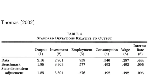
Differences from model-based predictions
Thomas (2002)
JOURNAL OF POLITICAL ECONOMY
TABLE 4
STANDARD DEVIATIONS RELATIVE TO OUTPUT
Output (1)
Investment
(2) Employment (3) Consumption (4) Wage (5) Interest
Rate (6)
Data 2.16 2.901 .959 .540 .287 .444
Benchmark 1.85 3.303 .577 .492 .492 .096
State-dependent
adjustment 1.85 3.304 .576 .492 .492 .095
Constant
adjustment 1.82 3.227 .556 .503 .503 .083
Partial adjustment 1.51 2.223 .305 .708 .708 .019
NOTE.-COI. 1 reports the percentage standard deviations for Hodrick-Prescott-filtered output in the data and the models. (Models are briefly summarized in table 3.) Cols. 2-6 are standard deviations relative to the standard deviation of output. In tables 4-7, the Hansen preference specification implies identical consumption and wage moments within each model economy.
what is perhaps more striking is that the inclusion of state-dependent lumpy investment patterns neither improves nor even affects model performance along any of these dimensions.
Table 4 reveals that the standard deviations for output, investment, employment, and consumption are essentially identical for the bench- mark and state-dependent adjustment economies. The similarities there extend to the constant adjustment model as well, which exhibits only somewhat reduced investment volatility. That closeness is further em- phasized by contrast to the traditional partial adjustment model, which exhibits a substantially weakened cycle because of excessively smooth investment demand. The overall similarity across models is also seen in the first- and second-order autocorrelations of table 6 and in the con- temporaneous and lagged correlations with output reported in tables 5 and 7. Consistent with its slightly reduced relative investment volatility, autocorrelations for the constant adjustment model's output, invest- ment, and employment series are somewhat higher, as are its investment and employment correlations with output.
The discussion above raises two questions. First, given that adjustment
TABLE 5
CONTEMPORANEOUS CORRELATIONS WITH OUTPUT
Investment
(1) Employment (2) Consumption (3) Wage
(4)
Interest Rate
(5)
Data .823 .903 .858 .263 -.385
Benchmark .973 .946 .924 .924 .889
State-dependent
adjustment .973 .946 .925 .925 .892
Constant adjustment .976 .950 .938 .938 .904
Partial adjustment .991 .971 .995 .995 .610
Motivation Discounting Discounting Plant-Level Optimization Results
Differences from model-based predictions
Thomas (2002)
JOURNAL OF POLITICAL ECONOMY
TABLE 4
STANDARD DEVIATIONS RELATIVE TO OUTPUT
Output (1)
Investment
(2) Employment (3) Consumption (4) Wage (5) Interest
Rate (6)
Data 2.16 2.901 .959 .540 .287 .444
Benchmark 1.85 3.303 .577 .492 .492 .096
State-dependent
adjustment 1.85 3.304 .576 .492 .492 .095
Constant
adjustment 1.82 3.227 .556 .503 .503 .083
Partial adjustment 1.51 2.223 .305 .708 .708 .019
NOTE.-COI. 1 reports the percentage standard deviations for Hodrick-Prescott-filtered output in the data and the models. (Models are briefly summarized in table 3.) Cols. 2-6 are standard deviations relative to the standard deviation of output. In tables 4-7, the Hansen preference specification implies identical consumption and wage moments within each model economy.
what is perhaps more striking is that the inclusion of state-dependent lumpy investment patterns neither improves nor even affects model performance along any of these dimensions.
Table 4 reveals that the standard deviations for output, investment, employment, and consumption are essentially identical for the bench- mark and state-dependent adjustment economies. The similarities there extend to the constant adjustment model as well, which exhibits only somewhat reduced investment volatility. That closeness is further em- phasized by contrast to the traditional partial adjustment model, which exhibits a substantially weakened cycle because of excessively smooth investment demand. The overall similarity across models is also seen in the first- and second-order autocorrelations of table 6 and in the con- temporaneous and lagged correlations with output reported in tables 5 and 7. Consistent with its slightly reduced relative investment volatility, autocorrelations for the constant adjustment model's output, invest- ment, and employment series are somewhat higher, as are its investment and employment correlations with output.
The discussion above raises two questions. First, given that adjustment
TABLE 5
CONTEMPORANEOUS CORRELATIONS WITH OUTPUT
Investment
(1) Employment (2) Consumption (3) Wage (4)
Interest Rate
(5)
Data .823 .903 .858 .263 -.385
Benchmark .973 .946 .924 .924 .889
State-dependent
adjustment .973 .946 .925 .925 .892
Constant adjustment .976 .950 .938 .938 .904
Partial adjustment .991 .971 .995 .995 .610
Motivation Discounting Discounting Plant-Level Optimization Results
Parameters:
From aggregate data (1948-2008)
ρA = 0.118 σA = 0.012
State-dependent discounting: ˆ
˜
βt+1 = 0.217ˆAt−0.507ˆAt+1
Motivation Discounting Discounting Plant-Level Optimization Results
Parameters:
From aggregate data (1948-2008)
ρA = 0.118 σA = 0.012
State-dependent discounting: ˆ
˜
βt+1 = 0.217ˆAt−0.507ˆAt+1