Development and Application of a New Positioning Algorithm for Wireless Sensor Networks

Development and Application of a New Positioning

Algorithm for Wireless Sensor Networks

https://doi.org/10.3991/ijoe.v14i10.9305

Guohong Gao(*₎

Henan Institute of Science and Technology, Xinxiang, China

[email protected]

Feng Wei

Xinxiang Vocational and Technical College, Xinxiang, China

Jianping Wang

Henan Institute of Science and Technology, Xinxiang, China

Abstract—This paper aims to create a desirable positioning method for nodes in wireless sensor networks (WSNs). For this purpose, a source node positioning algorithm was developed based on time-of-arrival (TOA), in view of the nonlin-ear correlation between the measured values and unknown parameters in the ob-servation equation of TOA source position. Several experiments were carried out to evaluate the performance of the proposed algorithm in terms of time measure-ment error, computing complexity, location error and Cramér–Rao lower bound (CRLB). The results show that the CRLB acquired by this algorithm can be used for WSN node positioning, provided that the independent zero mean Gauss meas-urement error is sufficiently small. The research findings lay a solid technical basis for optimal management, load balance, efficient routing, and automatic to-pology control of WSNs.

Keywords—wireless sensor networks, location algorithm, TOA, CRLB

1

Introduction

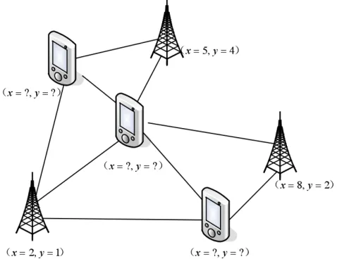
mobile location service industry has become one of the most promising mobile value-added services. Academic researchers often strive to achieve the most effective locali-zation methods under the current limited conditions of wireless devices and localilocali-zation systems. Figure 1 shows a localization problem. It should be pointed out that a general node can also be used as an anchor node, as long as it knows itself location.

In the WSNs node location, the performance of the evaluation location algorithm usually has the following evaluation criteria:

1.1 Location accuracy

In the WSNs location algorithm, the location accuracy is generally represented by the ratio of the error value to the wireless range of the node. In addition, some localiza-tion algorithms use the size of the two-dimensional network of the network to indicate its accuracy [2].

Fig. 1. Location problem of anchor node

1.2 Beacon node density

Another important indicator to measure the pros and cons of WSNs location algo-rithms is the density of reference nodes. Since the deployment of reference nodes in the WSNs manually or in a GPS mode has a great influence on the environment and appli-cation scalability of the WSNs, the reference node density can be used to evaluate one of the important indicators of the location algorithm cost and scalability [3].

1.3 Robustness and fault tolerance

location algorithms. In order to ensure that the location algorithm can be applied in the real environment and avoid problems such as multi-path transmission, non-line-of-sight, and communication blind spots, the WSNs location algorithm must have strong fault tolerance and adaptability [4].

1.4 Energy consumption

Considering the miniaturization and limited energy characteristics of WSNs, the en-ergy consumption problem is also one of the most important factors affecting the loca-tion algorithm. Therefore, for the localoca-tion of WSNs, trade-offs between localoca-tion accu-racy and energy consumption are also needed to be considered, making it possible to achieve a good balance between location accuracy and energy consumption [5].

According to the analysis of the above WSNs location algorithm performance indi-cators, in general, a better location algorithm should have higher location accuracy, lower reference node dependency, strong fault tolerance and robustness, and lower en-ergy consumption and the cost of realize and other characteristics [6-9]. These perfor-mance indicators are not only the perforperfor-mance indicators for evaluating WSNs' self-localization algorithms, but also the optimal targets for the research and design of loca-tion algorithms. In the WSNs localoca-tion problem, it is often necessary to comprehensively consider these performance indicators to make trade-offs based on specific require-ments and propose a location algorithm that applies to different scenarios and different standards.

2

Distance Measurement for Wireless Location

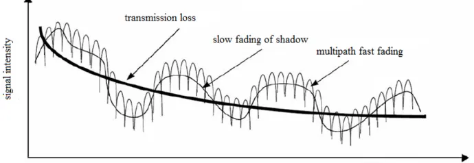
In general, the RSSI value of the wireless point is related to the transmission distance of the wireless signal. The closer the wireless communication distance, the larger the value is. The RSSI receiver is a terminal that accepts signal power size parameters. The signal it receives is a function of space, frequency, and time.

As shown in Figure 2, the change can be divided into path loss, shadow fading and small-scale fading. The path loss is the transmission loss caused by the distance be-tween the transmitter and the receiver, and the shadow fade is used to describe the change of the average signal intensity due to the diversity of the location environment. The small-scale fading is related to the signal strength characteristics of the shorter distance signal from the receiver.

The RSSI-based method uses a theoretical or empirical signal transmission attenua-tion model to convert the transmission loss to distance by comparing the radio signal strength received at the receiving point with the known radio frequency signal strength of the transmitting node. The signal attenuation model is generally expressed as follow:

𝑃𝑃(𝑑𝑑) = 𝑃𝑃(𝑑𝑑&) − 10 × 𝜂𝜂 × log /₀0₁2 − 3𝑛𝑛𝑛𝑛 × 𝑛𝑛𝑊𝑊𝑊𝑊 𝑛𝑛𝑛𝑛 ≤ 𝐶𝐶_{𝐶𝐶 × 𝑛𝑛𝑊𝑊𝑊𝑊 𝑛𝑛𝑛𝑛 ≥ 𝐶𝐶} (1)

where 𝑝𝑝(d) and p(d&) are the signal strengths at the distance from the base station

d and d& respectively.

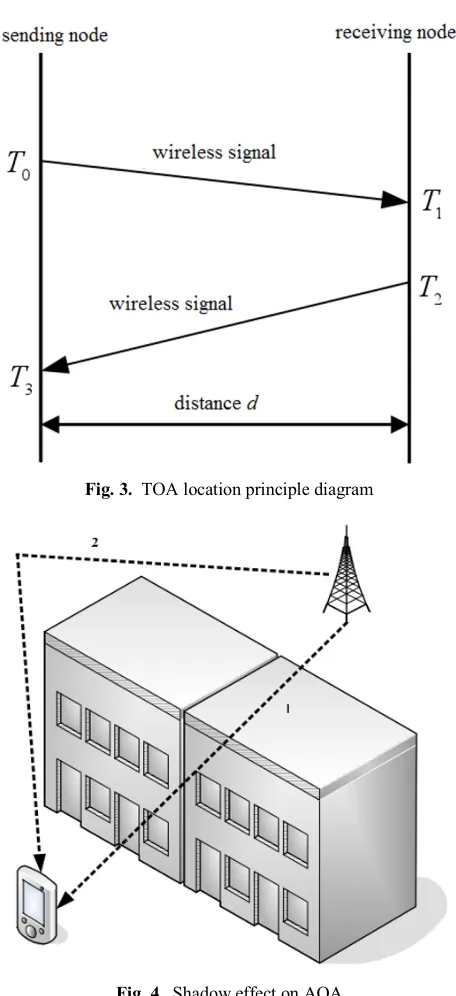
Since wireless sensors in general have wireless RF signals, it is easier to implement node ranging for the WSNs using the received signal strength. However, in the process of radio frequency signals achieving transmission, the signal attenuation due to envi-ronmental influences is inconsistent with the theoretical or empirical model and the individual differences of radio frequency hardware circuits. Therefore, ranging based on the received signal strength, and it is only a coarse-grained ranging technology [10]. The method obtains the distance by measuring the transmission time of the wireless transmission signal between the two nodes multiplied by its signal transmission speed, as shown in Figure 3. The signal is passed from the sending node to the receiving node, and then the receiving node sends another signal to send the node as a response. Through the "handshake" of both parties, the sending node can infer the distance from the node's periodic delay as follow:

d =?(@AB@1)B(@CB@D)E×F

G (2)

where 𝑉𝑉 represents the transmission speed of the wireless signal. The error of the meas-urement method mainly comes from the signal processing time, such as the calculation delay and the position delay 𝑇𝑇G− 𝑇𝑇J at the receiving end.

Fig. 3. TOA location principle diagram

Fig. 4. Shadow effect on AOA

estimate the position information of unknown nodes. There are some common geomet-ric methods, such as trilateration, triangulation, maximum likelihood estimation, hy-perbola, and hybrid location.

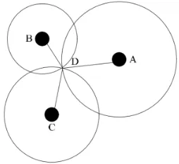
The following is a brief introduction to the trilateration method. In the location-based WSNs location algorithm, it is the most common and most basic method for calculating coordinates. The steps are as follows: Assume that the distance from the node D to the reference node A is ρJ, then D is on a circle with point A as the center and ρJas the

radius. Similarly, if the distance of unknown node D to two other reference nodes B

and C measured is 𝜌𝜌G, ρM. Then, point D is on a circle with B and C as its center and 𝜌𝜌G

and ρM as its radius. The way we can determine that the unknown node is at the

inter-sections of the three circles.

According to the geometric positions of the layouts A, B, C, and D shown in Figure 5, the coordinates of the three reference nodes A, B, and C are (xJ, yJ) , (xG, yG),

(xM, yM).

Fig. 5. Trilateration localization method

The distance between the unknown node D(x, y)and the three reference nodes is ρJ,

ρG, ρM, then

R

𝜌𝜌J= S(𝑥𝑥 − 𝑥𝑥J)G− (𝑦𝑦 − 𝑦𝑦J)G

𝜌𝜌G= S(𝑥𝑥 − 𝑥𝑥G)G− (𝑦𝑦 − 𝑦𝑦G)G

𝜌𝜌M= S(𝑥𝑥 − 𝑥𝑥M)G− (𝑦𝑦 − 𝑦𝑦M)G

(3)

Combined with the actual node geometry, the coordinates of node D can be solved

when assumed that there are no multiple solutions in Eq. (3).

V𝑥𝑥_{𝑦𝑦W = X}2(𝑥𝑥 − 𝑥𝑥J) 2(𝑦𝑦 − 𝑦𝑦M)

2(𝑥𝑥GB 𝑥𝑥M) 2(𝑦𝑦G− 𝑦𝑦M)Z BJ

X𝑥𝑥JG− 𝑥𝑥MG+ 𝑦𝑦JG− 𝑦𝑦MG+ 𝜌𝜌MG− 𝜌𝜌JG

𝑥𝑥GG− 𝑥𝑥MG+ 𝑦𝑦GG− 𝑦𝑦MG+ 𝜌𝜌MG− 𝜌𝜌GGZ (4)

3

TOA-based Source Localization Algorithm by Using

Coordinate Translation Linearization

3.1 Algorithmic signal data model

In two-dimensional coordinate systems, a position can be represented by a column vector consisting of two elements. It is generally considered that a two-dimensional scheme can be described as follows: a signal emitting source node whose unknown position is denoted as p& and a timing for transmitting the timing signal as t&. There

are m sensor nodes that are in sync with each other, and their known positions are de-noted as 𝑝𝑝^, 𝑚𝑚 = 1, ⋯ , 𝑀𝑀. The TOA measured as the arrival time of the corresponding

sensor is recorded as tb, 𝑚𝑚 = 1, ⋯ , 𝑀𝑀. All the observation equations are expressed as

follows:

𝑡𝑡^= 𝑡𝑡&+J_d‖𝑝𝑝&− 𝑝𝑝^‖ + 𝑛𝑛^, 𝑚𝑚 = 1, ⋯ , 𝑀𝑀 (5)

where c is the known speed of transmission. Although 𝑡𝑡& can be estimated at the same

time, we only considers the estimate of 𝑝𝑝&. Let the estimated position of the source node

be 𝑝𝑝&, a suitable performance indicator is the mean square error (m.s.) location error.

m. locazation error = E{‖𝑝𝑝̂&− 𝑝𝑝&‖G} (6)

In the case of sufficiently small Gaussian zero mean and independent measurement error, the above-mentioned mean square error location error is limited by the CRLB. CRLB can be derived from the probability density function given all unknown TOA measurement data and sensor locations.

The corresponding probability density function of the observation equation is ex-pressed as follows:

f(𝑡𝑡J, ⋯ , 𝑡𝑡^|𝑡𝑡&,𝑝𝑝&, 𝑝𝑝J⋯ 𝑝𝑝t) =_S(GuvJ

wC)w𝑒𝑒𝑥𝑥𝑝𝑝 V−

J

GvwC∑ /𝑡𝑡&− 𝑡𝑡^+

J d‖𝑝𝑝&− t

^BJ

𝑝𝑝^‖2W G

(7)

The corresponding Fisher information matrix is

I = −E {|

}C }~1}~1ln 𝑓𝑓

}C }Å1}~1ln 𝑓𝑓

}C }~1}Å1ln 𝑓𝑓

}C }C_Å1ln 𝑓𝑓

ÇÉ (8)

Where

−E 3_}~}C

1}~1ln 𝑓𝑓Ñ =

J vwC∑

(~1B~Ö)(~1B~Ö)

‖~1B~Ö‖

t

^BJ (9)

−E 3_}}CC_Å1ln 𝑓𝑓Ñ =

t

−E 3_}~}C

1}Å1ln 𝑓𝑓Ñ =

J dvwC∑

(~1B~Ö)

‖~1B~Ö‖

t

^BJ (11)

So CRLB is

CRLB = TR{𝐈𝐈BJ_{} (12)}

3.2 Source location algorithm

Prior to the first stage of the evaluation algorithm presented in this paper, a suitable translation of the coordinate system is performed firstly, and the origin of the coordinate system is translated to the closest sensor node from the unknown source node, that is, the received time is the shortest (measured according to TOA). If the corresponding sensor node is labeled as sensor k, the above coordinate system transformation is ex-pressed as follows:

𝑃𝑃åç= 𝑃𝑃å− 𝑃𝑃é, 𝑖𝑖 = 0,1, ⋯ , 𝑀𝑀 (13)

𝑡𝑡åç= 𝑡𝑡å− 𝑡𝑡é,𝑖𝑖 = 0,1, ⋯ , 𝑀𝑀 (14)

Where

k = argmin^𝑡𝑡^ (15)

After transformation of the coordinate system, the following equation is obtained:

ë𝑝𝑝ç ^ë

G

− 𝑐𝑐G_𝑡𝑡ç

^G= 2𝑝𝑝ç_^@𝑝𝑝ç_&− 2𝑐𝑐G𝑡𝑡ç^𝑡𝑡ç&− /ë𝑝𝑝ç_&ëG− 𝑐𝑐G𝑡𝑡ç&G2 + 2𝑐𝑐G(𝑡𝑡ç&−

𝑡𝑡ç

^)𝑛𝑛^+ 𝑐𝑐G𝑛𝑛^G,𝑚𝑚 = 1, ⋯ , 𝑀𝑀 (16)

In view of the above coordinate transformation, in observation Eq. (5), when m = k, it becomes

0 = 𝑡𝑡ç

&+J_d‖𝑃𝑃ç‖ + 𝑛𝑛é (17)

So, it can be deduced

ë𝑝𝑝ç &ë

G

− 𝑐𝑐G_𝑡𝑡ç

&G= 2𝑐𝑐G𝑡𝑡ç&𝑛𝑛é+ 𝑐𝑐G𝑛𝑛éG (18)

Then we can see that the right side of the above equation contains only the relevant items of measurement error. The transformed observation equations appear in the form of a matrix.

ì ‖P

ç_‖G_{− c}G_t JçG

⋮ ‖pñç‖G− cGtñçG

ó = ì2pJ

çò _−2cG_t Jç

⋮ ⋮ 1⋮

2pñçò −2cGtñç 1

ó XP&ç

t&çZ +

ô −2c

G_t

&çnö− cGnöG− 2cG(t&ç− tJç)nJ+ cGnJG

⋮ −2cG_t

&çnö− cGnöG− 2cG(t&ç− tñç)nñ+ cGnñG

Or it can be simply expressed as

𝑏𝑏ç_{= 𝑊𝑊}ç_𝑞𝑞ç_{+ 𝑤𝑤}ç ₍₂₀₎

From the above formula, it can be seen that the nonlinearity has been eliminated. Since the error variance of the above equation is unknown at the first stage, the LS solution with the same weight is used here.

𝑞𝑞üç_{= (𝑊𝑊}ç@_𝑊𝑊ç₎BJ_𝑊𝑊ç@_𝑏𝑏ç_{= †}𝑝𝑝̂&ç

𝑡𝑡̂&ç° (21)

It can be seen from the above equation that when there is no measurement error, the above estimated unknowns, namely pü&ç and t̂&ç, must be correct values.

Prior to the second stage evaluation, the corresponding coordinate system transfor-mation still needs to be performed. The coordinate system origin is again converted to the estimated position and converted estimate the estimated transmission time to the source node in the first stage evaluation.

𝑝𝑝åçç= 𝑝𝑝åç− 𝑝𝑝̂&ç, 𝑖𝑖 = 0,1, ⋯ , 𝑀𝑀 (22)

And

𝑡𝑡åçç= 𝑡𝑡åç− 𝑡𝑡̂&ç, 𝑖𝑖 = 0,1, ⋯ , 𝑀𝑀 (23)

It can be seen that p¢çç and t¢çç contain only the items of measurement error.

After converting the coordinate system, the observation Eq. (16) becomes

ë𝑝𝑝çç ^ë

G

− 𝑐𝑐G_𝑡𝑡çç

^G= 2𝑝𝑝çç^@𝑝𝑝çç&− 2𝑐𝑐G𝑡𝑡çç^𝑡𝑡çç&− /ë𝑝𝑝çç&ë G

− 𝑐𝑐G_𝑡𝑡çç

&G2 + 2𝑐𝑐G(𝑡𝑡çç&−

𝑡𝑡çç

^)𝑛𝑛^+ 𝑐𝑐G𝑛𝑛^G,𝑚𝑚 = 1, ⋯ , 𝑀𝑀 (24)

After the transformation of the coordinate system, p¢çç, t¢çç only contains items with

measurement errors. Therefore, when the measurement error is sufficiently small, the

ëpçç &ë

G

term contains only the second-order measurement error, which is negligible compared to the simultaneous presence of the 2pçç

bòpçç& term in Eq. (24). Similarly,

the cG_tçç

&G term contains only the second-order measurement error term, which is

neg-ligible compared to the coexistence term 2cG_tçç

btçç& in Eq. (24). Therefore, when the

measurement error is small enough, in Eq. (24), the item ëpçç &ë

G

− cG_tçç

&G can be

ig-nored. In the following, specific proofs about why ëpçç &ë

G

and cG_tçç

&G can be omitted.

Here, cG_tçç

&G is took concrete derivation example. The above conclusion immediately

corresponds to a value that needs to prove that cG_tçç

&G is insignificant with respect to

2cG_tçç btçç&.

Consider the following scenario, it has a fixed value c and tçç

b, and an estimated

error tçç

& that satisfies zero mean. If the variance is a Gaussian distribution of σG, which

p = †_G|d•dCC_Ŷ¶ÖŶ¶1C_Ŷ¶1• _|< 𝜀𝜀° (25)

where ε is a fixed positive number, f it is a critical value of a negligible denominator. For example, a critical value of ε = 0.01 will be a sufficient condition for cG_tçç

&G to

ignore for many practical scenarios. And this situation is equivalent to the proof of the following equation:

p = †_G|d•dCC_Ŷ¶ÖŶ¶1C_Ŷ¶1• _|< 𝜀𝜀° → 1 (26)

When estimating the variance σG_{→ 0 of the error, Eq. (26) can be written as}

p(|𝑡𝑡çç

&| < 2|𝑡𝑡çç^|𝜀𝜀) = 1 − 𝑒𝑒𝑥𝑥𝑝𝑝 ´G¨Å

¶¶ Ö¨C≠C

vC Æ (27)

According to the cumulative distribution function of the Rayleigh distribution, we can observe Eq. (27) for any fixed value s, by reducing σG _{up to 0, the following results}

can be obtained.

p = †_G|d•d_CC_Ŷ¶ÖŶ¶1C_Ŷ¶1• _|° → 1 (28)

The Eq. (28) is equivalent to the fact that the ¨cG_tçç

&G¨ term is irrelevant to the

2|cG_tçç

btçç&| term.

Therefore, when the measurement error is small enough, Eq. (24) can be approxi-mated as follows:

ë𝑝𝑝çç ^ë

G

− 𝑐𝑐G_𝑡𝑡çç

^G≈ 2𝑝𝑝çç^@𝑝𝑝çç&− 2𝑐𝑐G𝑡𝑡çç^𝑡𝑡çç&− 2𝑐𝑐G𝑡𝑡çç^𝑛𝑛^,𝑚𝑚 = 1, ⋯ , 𝑀𝑀 (29)

or in the form of a vector matrix as follows:

ì ‖𝑃𝑃

çç_‖G_{− 𝑐𝑐}G_𝑡𝑡 JççG

⋮

‖𝑝𝑝tçç‖G− 𝑐𝑐G𝑡𝑡tççG

ó ≈ ì2𝑝𝑝J

çç@

⋮ −2𝑐𝑐

G_𝑡𝑡 Jç′

⋮ 2𝑝𝑝tçç@ −2𝑐𝑐G𝑡𝑡tç′

ó X𝑃𝑃&çç

𝑡𝑡&ççZ + ô

−2𝑐𝑐G_𝑡𝑡 Jçç𝑛𝑛J

⋮ −2𝑐𝑐G_𝑡𝑡

tçç𝑛𝑛t

õ (30)

It can be simply expressed as:

𝑏𝑏çç_{= 𝑊𝑊}ç_′𝑞𝑞çç_{+ 𝑤𝑤}çç ₍₃₁₎

Using known approximate weights, the WLS solution becomes

𝑞𝑞üçç_{= (𝑊𝑊}çç@_𝑛𝑛ççBJ_𝑊𝑊çç₎BJ_𝑊𝑊ç@_𝑛𝑛ççBJ_𝑏𝑏çç_{= †}𝑝𝑝̂&çç

𝑡𝑡̂&çç° (32)

Where

𝑛𝑛çç_{= 𝑑𝑑𝑖𝑖𝑑𝑑𝑑𝑑{[4𝑐𝑐}µ_𝑡𝑡

After the above two stages of estimation, coordinate system transformation will be performed again to restore the original coordinate system.

𝑝𝑝̂&= 𝑝𝑝̂&çç+ 𝑝𝑝̂&ç+ 𝑝𝑝é (34)

𝑡𝑡̂&= 𝑡𝑡̂&çç+ 𝑡𝑡̂&ç+ 𝑡𝑡é (35)

4

Simulation Analysis

The specific performance of the proposed TOA-based source location algorithm is evaluated through simulation. First, assume that the source node and the five sensor nodes in the sensor network are randomly distributed in one [-300, -300], [-300, 300], [300, 300], [300, -300] are the square regions of the vertices, and the signal transmission times of the source nodes are randomly distributed in the time period [-1000, 1000] (in nanoseconds). The TOA measurement error is assumed to be Gaussian zero mean error and independent of each other.

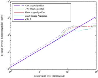
Figure 6 shows the position of the randomly generated source sensor and the source transmission time during simulation and is fixed. It obtains curves from an average of more than 1000 independent runs and all measurement errors are generated inde-pendently in each run.

As can be observed from Figure 6, the two-stage location algorithm proposed in this paper is superior to the one-stage location algorithm. When the measurement error is small enough, the CRLB lower limit can be approached. When the measurement error is relatively large, the third-stage algorithm achieves a slightly better location perfor-mance than the second-order algorithm. The convergence characteristics of the subse-quent two-stage algorithm with iterative LS minimization are also slightly better than the two-stage algorithm.

Figure 7 shows that the position of the randomly generated source sensor and the source emission time are not fixed in the simulation process. It derives curves from an average of more than 1000 independent executions, but measure error in each inde-pendent execution, source sensor position and source emission time are generated in-dependently.

Fig. 7. The simulated localization error against the measurement error

5

Conclusions

This chapter proposes a method of locating an unknown signal source based on the signal arrival time (TOA) measured by an unknown node of the sensor, where the po-sitions of other sensor nodes are known and synchronized with the time of the unknown nodes. In general, the corresponding observation equation based on TOA source loca-tion includes the nonlinear relaloca-tionship between measured values and unknown param-eters. It will get result in the absence of valid unbiased estimates that approximate CRLB. A corresponding source localization algorithm based on TOA for linearization using coordinate system translation is proposed. The performance of the algorithm was evaluated in terms of time measurement error, computational complexity, mean squared location error, and CRLB. The simulation study of the location algorithm shows that when the independent zero-mean Gaussian measurement error is assumed to be small enough, the proposed location algorithm can effectively approach the CRLB lower limit value. It is applicable to the WSNs node location system based on the TOA measure-ment model.

6

References

[1]Gui, L., Val, T., Wei, A. (2015). Improvement of range-free localization technology by a novel DV-hop protocol in wireless sensor networks. Ad Hoc Networks, 24(7): 55-73.

https://doi.org/10.1016/j.adhoc.2014.07.025

[2]Liu, K., Chen, L., Liu, Y. (2008). Robust and Efficient Aggregate Query Processing in Wire-less Sensor Networks. Mobile Networks & Applications, 13(1): 212-227.

https://doi.org/10.1007/s11036-008-0052-6

[3]Zhao, F., Ma, Y., Luo, H.Y. (2009). A mobile beacon-assisted node localization algo-rithm using network-density-based clustering for wireless sensor networks. Journal of Electronics & Information Technology, 31(12): 2988-2992.

[4]Pei, Z., Deng, Z., Xu, S. (2009). Anchor-Free Localization Method for Mobile Targets in Coal Mine Wireless Sensor Networks. Sensors, 9(4): 2836-2850. https://doi.org/10.3390/ s90402836

[5]Liu, M.G.X. (2011). Distributed Data Fusion Algorithm with Low Energy Consump-tion and High Accuracy in WSN. International Journal of Advancements in Compu-ting Tech-nology, 3(11): 122-129. https://doi.org/10.4156/ijact.vol3.issue11.16

[6]Zhan, J., Liu, H.L., Huang, B.W. (2011). A New Algorithm of Mobile Node Localiza-tion Based on RSSI. Wireless Engineering & Technology, 2(2): 112-117.

https://doi.org/10.4236/wet.2011.22016

[7]Chidean, M.I., Morgado, E., Sanromán-Junquera, M. Energy Efficiency and Quality of Data Reconstruction Through Data-Coupled Clustering for Self-Organized Large-Scale WSNs. IEEE Sensors Journal, 16(12): 5010-5020. https://doi.org/10.1109/JSEN.2016.2551466

[8]Bai, L.Q., Ling, L.I., Qian, S.G. (2017). Source-location privacy protection algorithm in WSNs based on ellipse model. Control & Decision 2017; 32(2): 255-261.

[10]Wang, B., Shi, L., Ren, F.Y. (2005). Self-Localization Systems and Algorithms for Wireless Sensor Networks. Journal of Software, 16(5): 857-862. https://doi.org/10.1360/jos160857

[11]Yun, Y.U., Choi, J.K., Yoo, S.J. (2011). Location-Based Spiral Clustering Algorithm for Avoiding Inter-Cluster Collisions in WSNs. Ksii Transactions on Internet & In-formation Systems 2011; 5(5): 665-683. https://doi.org/10.3837/tiis.2011.04.003

7

Authors

Guohong Gao received his bachelor's degree in Computer Application Technology from Henan Normal University, Xinxiang, Henan, China, in 2000, the master's degree in Computer Application Technology from Huazhong University of Science and Tech-nology, Wuhan, China, in 2008. He is now a lecturer at School of Information Engi-neering, Henan Institute of Science and Technology, Xinxiang, China. His current re-search interests include cloud computing, Internet of things technology and applica-tions.

Feng Wei received his bachelor's degree in Computer Science and Technology from Zhengzhou University of Aeronautics, Zhengzhou, Henan, China, in 2004, the master's degree in Agricultural Informatization from Henan Normal University, Xinxiang, He-nan, China, in 2015. He is now a lecturer at Xinxiang Vocational and Technical Col-lege, Xinxiang, China. His current research interests include pattern recognition, image processing, neural networks, natural language processing.

Jianping Wang received his bachelor's degree in computer science and technology from Shanxi Normal University, Xinxiang, Henan, China, in 2004. He is now a lecturer at School of Information Engineering, Henan Institute of Science and Technology, Xinxiang, China. His current research interests include SDN network of underwater sensors.