30 mm
Pantone 281U Pantone Warm Gray 7 U
Colori versione positiva Doctoral School in Cognitive and Brain Sciences XXVI Cycle
Doctoral Thesis
Distributional semantic phrases
vs. semantic distributional nonsense:
Adjective Modification in
Compositional Distributional Semantics
Eva Maria Vecchi
Advisors: Prof. Roberto Zamparelli Prof. Marco Baroni
There are so many people to acknowledge for the sweat and tears that has been put into the work of this thesis, it is hard to know where to begin. A whole chapter should be written just to thank my supportive and extremely patient advisors: Roberto Zamparelli, whose creative insight and intelligence has forced open doors in my research that I never thought possible, and Marco Baroni, whose work ethic, curiosity and determination has encouraged me to push myself to always learn, question and explore more each day. They have each taught me so much during these years, and I am a better researcher and person for this. I thank them both for their encouragement, advice and friendship throughout my Ph.D. career.
I would like to thank my Oversight Committee, particularly Raffaella Bernardi and Marco Marelli, for their time and invaluable suggestions. Thank you to Gemma Boleda and Louise McNally for their contribu-tion to my work, my scientific interest and growth. It has been an incredible pleasure working with you.
A very special thanks are dedicated to both Andrew Anderson, who has been a rock for me through it all, and Elia Bruni for his infinite patience and advice during these three years (even when I never get it right: “ventolaio”!).
Parts of this thesis (ideas, figures, results and discussions) have appeared previ-ously in the following publications:
Vecchi, E.M., Baroni, M. & Zamparelli, R. (2011). (Linear) maps of the impossible: Capturing semantic anomalies in distributional space. InProceedings of the ACL Workshop on Distributional Semantics and Compositionality, 1–9, Portland, OR.
Boleda, G.,Vecchi, E.M.,Cornudella, M.&McNally, L.(2012). First-order vs. higher-First-order modification in distributional semantics. In Proceedings of the 2012 Joint Conference on EMNLP and CoNLL, 1223–1233, Jeju Island, Korea.
Vecchi, E.M., Marelli, M., Zamparelli, R. &Baroni, M. (2013). Spicy adjectives and nominal donkeys: Capturing semantic deviance using composi-tionality in distributional spaces. In Review.
Contents v
List of Figures vii
List of Tables viii
1 Introduction 1
2 General experimental design 9
2.1 Semantic space . . . 9
2.2 Composition models . . . 15
3 Degrees of adjective modification in distributional semantics 19 3.1 Introduction . . . 19
3.2 The semantics of adjectival modification . . . 21
3.3 Methodology . . . 24
3.4 Results . . . 26
3.5 Discussion . . . 34
4 Capturing semantic deviance 36 4.1 Introduction . . . 36
4.2 Related work . . . 40
4.3 Experiment 1: Pilot Study . . . 46
5 Behavior of recursive adjective modification 75
5.1 Introduction . . . 75
5.2 The syntax of adjectives . . . 77
5.3 Materials and methods . . . 82
5.4 Results . . . 91
5.5 Discussion . . . 97
6 Conclusions 100 Appendix A 104 A.1 Access to datasets . . . 104
A.2 Evaluation materials . . . 104
3.1 Cosine distance distribution across the three types of AN phrases:
intersective, subsective and intensional. . . 27
4.1 Distribution of acceptability judgments of unattested ANs. . . 56
4.2 Prediction for plausibility measure: Cosine . . . 59
4.3 Prediction for plausibility measure: Vector length . . . 59
4.4 Prediction for plausibility measure: Density . . . 61
4.5 Prediction for plausibility measure: Entropy . . . 62
4.6 Prediction for plausibility measure: Adjective densification . . . . 63
A.2.1Screenshot of the instructions presented to the contributors of the CF task. . . 105
2.1 Semantic space parameter tuning . . . 14
2.2 Composed space quality evaluation . . . 18
3.1 Example intersective, subsective and intensional ANs in the dataset 25 3.2 Results of intersective vs. subsective color terms . . . 30
3.3 Nearest neighbors for color terms . . . 32
3.4 Results of intersective vs. intensional ANs . . . 33
3.5 Nearest neighbors for intensional terms . . . 34
4.1 Difference between acceptable and deviant ANs . . . 49
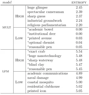
4.2 Highest/lowest entropy scores for significant models I . . . 50
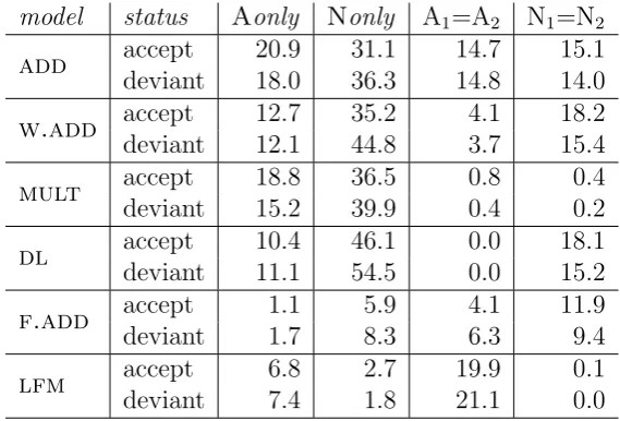
4.3 Percentage distributions of top 10 neighbors . . . 51
4.4 Results of the effect of word-based measures on the choice of ac-ceptability . . . 65
4.5 Improvement on word-based measures . . . 67
4.6 Results on distributional semantic measures . . . 68
4.7 Highest/lowest entropy scores for significant models II . . . 71
4.8 Examples of the nearest neighbors of model-generated ANs . . . . 73
5.1 Examples of the nearest neighbors of the gold standard for flexible order and rigid order AANs. . . 90
5.2 Mean cosine similarities for gold AANs . . . 91
5.3 Flexible vs. rigid order AANs . . . 93
Introduction
In this thesis, I study the ability of compositional distributional semantics to model adjective modification. In particular, I am interested in how such statisti-cal approaches to meaning representation are able to approximate both the intu-ition of natural language speakers and the knowledge we have gained throughout generations of theoretical research on this topic.
The general aim of this research is twofold. First, I investigate how com-positional distributional semantics of adjective-noun phrases is able to capture linguistic phenomena that have been concluded in previous literature. For exam-ple, a coherent model of adjective-noun semantics should be able to handle the difference between the degree of modification of the word white in the phrases white shirt,white wine and white lie. Further, strong evidence has been provided for the effects of adjective semantics on ordering restrictions in recursive mod-ification. Ideally, models that properly model the semantics of adjective-noun phrases should encompass inherent properties that support this evidence.
even though they seem to share no properties, I would like to point out that both phrases are never found (or unattested) in an extremely large and comprehen-sive corpus, although their constituents are all found extremely frequently in the same corpus. The idea of what makes a novel phrase acceptable or unacceptable is interesting in many respects, and many fields can benefit from such knowl-edge (see Chapter 4 for more discussion). My goal is to exploit the properties of the distributional representations of such phrases to be able to gain a better understanding of this issue.
Semantics is the cognitive faculty that allows us to use language to reason and communicate about states of the world and of our minds (Chierchia & McConnell-Ginet, 2000). A number of fields have long sought to devise an artificial system endowed with human-like capabilities to understand and use natural language semantics. Researchers working on the development of this topic have explored a number of approaches to establish a system capable of this task. Although the approaches have varied a bit, the aims of such a system are consistent. First, it should be able to model semantic representations for naturally occurring text on a large scale. Second, the system should understand and incorporate the compo-sitional aspect of natural language in order to combine words to construct and interpret sentences that have not yet been encountered by the system. Finally, it should agree with and even emulate human behaviour and intuition on a variety of semantic tasks.
Such a system that has the ability to retrieve and manipulate meaning could benefit a multitude of fields. In Cognitive Science, for example, it could aid in tasks such as Memory Retrieval, Categorization, Problem Solving, Reasoning and Learning. While in Theoretical Linguistics, it could promise a wider coverage of semantic analysis and free it of unrealistic idealizations. Natural Language Pro-cessing (NLP) could benefit from such a system in tasks like Question-Answering, Information Retrieval and Machine Translation.
– specifically, shorter paths for semantically related words.
However, this approach has been criticized as accounting for an idealized representation that is not completely in sync with real-world usage (Mitchell & Lapata, 2010). This criticism is based on the fact that the represenations are hand-coded by human modelers who a priori determine which relationships are most relevant in representing meaning. Attempts ot create semantic networks from word association norms (Steyvers & Tenenbaum, 2005) have aimed to over-come this, however they can only represent a small fraction of the vocabulary of an adult speaker.
An alternative to semantic networks exploit the idea that word meaning can be described in terms of feature lists (Smith & Medin, 1981). Specifically, each word is represented by a distribution of numerical values over a feature set. Although norming studies have the potential of revealing which dimensions of meaning are psychologically salient, working with such data gives rise to a number of difficulties such as the varying number and type of attributes generated, the large degree of freedom in the way responses are coded and analyzed, and asking multiple subjects to create a representation for each word limits the studies to a small-sized lexicon.
Another approach to natural language semantics, based on Montague Gram-mar (Montague, 1974), is built on predicate logic and lambda calculus. Such formal approaches are truth-conditional and model theoretic; that is, the mean-ing of a sentence is represented by its truth conditions which are expressed in terms of truth relative to some model of the world. In other words, a language is mapped onto a set of possible worlds, and other semantical notions are de-fined as functions on individuals and possible worlds. The meanings of referring expressions are taken to be entities/individuals in the model and predicates are functions from entities to truth-values (i.e. the meanings of propositions). These functions can also be characterised in an ‘external’ way in terms of sets in the model – this extended notion of reference is usually called denotation.
car-ried out syntactically (see below for further discussion on Formal Semantics and Compositionality). However, a drawback of this approach is that it lacks fine-grained representations for content words (such as adjectives and nouns), which is a centerpiece and advantage in other models. Such an approach also relies on ambiguous inputs, leading to expensive computations to compute all possible readings.
Distributional Semantic Models An approach to semantic representation that has gained a lot of attention in recent work, Distributional Semantic Models (DSMs), is based on the assumption that word meaning can be learned from the linguistic environment. According to the “distributional hypothesis of meaning” (Harris, 1968), words that are similar in meaning tend to occur in contexts of similar words, and thus meaning is susceptible to distributional analysis. DSMs aim to capture meaning quantitatively in terms of co-occurrence statistics from large collections of text, or corpora. Words are represented as vectors in a high-dimensional space, where each component corresponds to some co-occurring con-textual element (Turney & Pantel, 2010).
An example implementation of this approach is the Hyperspace Analog to Language model (HAL, Lund & Burgess, 1996). In this model, each word is rep-resented by a vector where each element of the vector corresponds to a weighted co-occurrence value of that word with some other word. Latent Semantic Analysis (LSA, Landauer & Dumais, 1997) also derives a high-dimensional space for words while using co-occurrence information between words and the passages they occur in. Both models are pioneer data-driven and wide-coverage DSM systems.
its extensions, such as probabilistic topic models (Bleiet al., 2003; Griffithset al., 2007)) have also proved successful at simulating a wide range of psycholinguistic phenomena, for example, semantic priming (Griffithset al., 2007; Landauer & Du-mais, 1997; Lund & Burgess, 1996), word categorization (Laham, 2000), reading times (Griffiths et al., 2007; McDonald, 2000), and judgments of semantic sim-ilarity (McDonald, 2000) and association (Denhi`ere & Lemaire, 2004; Griffiths et al., 2007). However, approaches that model semantic meaning this way are not naturally compositional, and most often vectors are combined by approaches that are insensitive to word order and syntactic structure.
Formal semantics and compositionality Speakers of a natural language are able to understand infinitely many sentences with different meanings. In fact, we are able to understand and produce sentences that have never before been heard or expressed based on our knowledge of the language. This productive capacity has been accredited to the compositional nature of natural language, a crucial property that allows us to derive the meaning of a complex linguistic constituent from the meaning of its immediate syntactic subconstituents (Frege, 1892; Partee, 2004).
Above, I introduced an approach to semantic representation based on predi-cate logic and lambda calculus. Logic-based frameworks in Formal Semantics (FS, Montague, 1974) are founded on the premise that there exists no theoretically relevant difference between artificial (formal) and natural (human) languages. In consequence, we can model logical structures of natural languages by means of universal algebra and mathematical (formal) logic. This framework is parallel to a syntactic system in which simple structures are put together into complex structures (Categorical Grammar) complex meanings are also constructed from simple meanings. FS aims to obtain first-order logic (FoL) representations of the meaning of a phrase compositionally through function application following the syntactic structure.
of the meaning of the parts and of the way they are syntactically combined. In other words, each syntactic operation of a formal language should have a corresponding semantic operation. This concept is illustrated in examples (1) and (2) from Landauer et al. (1997).
(1) It was not the sales manager who hit the bottle that day, but the office worker with the serious drinking problem.
(2) That day the office manager, who was drinking, hit the problem sales worker with the bottle, but it was not serious.
Compositionality is a matter of degree rather than a binary notion since linguistic structures range across levels of compositionality (Nunberget al., 1994). In simple cases, the meaning of an expression can be considered fully compositional, such as attributive adjective-noun phrases in which the meaning is the intersection of the meaning of the adjective and the noun, such as red car. Syntactically fixed expressions, such as take advantage, are only partly compositional because the constituents can still be assigned separate meanings. Certain idioms, such as kick the bucket, or multiword expressions, such as by and large, are considered much less compositional since their meaning cannot be distributed across their constituents.
Compositional distributional semantics
Semantic representations of single words can be represented as vectors in high-dimensional DSMs. By exploiting the geometric nature of these representa-tions, given two independent vectors v1 andv2 in the space, we can then combine
the independent vectors to produce a semantically compositional result v3.
At-tempts in this task have explored a number of possible operations to combine these vectors, described in detail below. We can measure the success of such ap-proaches in terms of their ability to model semantic properties of simple phrases, in tasks such as phrase similarity (Baroni & Zamparelli, 2010; Erk & Pad´o, 2008; Grefenstette & Sadrzadeh, 2011b; Mitchell & Lapata, 2010), textual entailment, semantic plausibility analysis (Vecchiet al., 2011), and sentiment analysis (Socher et al., 2011).
For the experiments presented in this thesis, we focus on various composition models in recent literature. The models and their parameter settings used in these experiments are described in detail in Section 2.2.
Outline
The thesis is structured as follows. In Chapter 2, I present a general framework for the experimental design which is then implemented in all experiments pre-sented here. In this chapter, I describe the construction of the semantic space (Section 2.1) as well as the parameter tuning of the space (Section 2.1.4). In ad-dition, I provide a general description of the implementation of each composition model (Section 2.2) and, again, provide details about the parameter estimation for each model (Section 2.2.1).
Chapter 3 introduces an experiment in which I use distributional semantic methods to detect differences in degrees of modification. I introduce the study with an overview of adjective semantics (Section 3.2). I then present the materials and methodology used to explore the research question (Section 3.3), and finally I provide an analysis of the results of the experiments (Section 3.4) and discussion (Section 3.5).
question of “unattestedness” and semantic deviance (Section 4.1) and a descrip-tion of related work on the topic (Secdescrip-tion 4.2). I then present two studies to explore the issue. In Section 4.3, I introduce a pilot study which tests the fea-sibility of detecting semantic deviance and introduces preliminary measures. I present an analysis for these results (Section 4.3.3) and open the door for a more extensive study (Section 4.3.4). Section 4.4 introduces the extended study, pro-viding a comparison to previous psycholinguistic analysis of acceptability of novel phrases. In this study, I expand the plausibility dataset to cover phrases contain-ing nearly 700 adjectives (Section 4.4.1), and expand on the preliminary measures for semantic deviance (Section 4.4.2). I then analyze the results (Section 4.4.3) and conclude with a discussion (Section 4.4.4).
Chapter 5 is a study of the behavior of adjectives in recursive modification. I apply compositional models recursively (Section 5.3.2) to generate distributional representations of complex adjective-noun phrases, and extract information using these representation to gain a better understanding of adjective ordering restric-tions. I construct an evaluation set of recursive adjective phrases (Section 5.3.4) and introduce measures to detect order restrictions (Section 5.3.3). The results are analyzed in detail (Section 5.4) and I close the chapter with a discussion and ideas for future work (Section 5.5).
General experimental design
2.1
Semantic space
Our initial step was to construct asemantic space for our experiments, consisting of a matrix where each row represents the meaning of an adjective, noun or AN as a distributional vector. I first introduce the source corpus, then the vocabulary of words and ANs that I represent in the space, and finally the procedure adopted to build the vectors representing the vocabulary items from corpus statistics, and obtain the semantic space matrix. I work here with a “vanilla” semantic space (essentially, following the steps of Baroni & Zamparelli 2010), since our focus is on the effect of different composition methods given a common semantic space. In addition, Blacoe & Lapata (2012) found that a vanilla space of this sort performed best in their experiments.
2.1.1
Source corpus
plural-ization and verb inflection.
2.1.2
Semantic space vocabulary
The words and phrases in the semantic space must of course include the items that I need for our experiments (adjectives, nouns and ANs used for model train-ing, as input to composition and for evaluation). Moreover, in order to study the behavior of the test items I are interested in (that is, model-generated AN vectors) within a large and less ad-hoc space I also include many more adjec-tives, nouns and ANs in our vocabulary not directly relevant to our experimental manipulations.
I first populate our semantic space with a core vocabulary containing the 8K most frequent nouns and the 4K most frequent adjectives from the corpus. In order to compare our experimental procedure to standard similarity judgment datasets, I included any adjective and noun used in Rubenstein & Goodenough (1965) and Mitchell & Lapata (2010). The vocabulary was then extended to include a large set of ANs (119K cumulatively), for a total of 132K vocabulary items in the semantic space.
To create the ANs needed to run and evaluate the experiments described below, I focused on adjectives which are very frequent in the corpus so that they generally be able to combine with many classes of nouns. I therefore define a
target vocabularycontaining the 700 most frequent adjectives and the 4K most frequent nouns in the corpus. Before generating the ANs, I manually controlled the target adjectives and nouns for problematic cases —adjectives such as above, less, or very, and nouns such as cant, mph, oryours – often due to parsing errors in the corpus. The ANs were generated by crossing the target nouns with the filtered 663 target adjectives and the filtered 3,910 target nouns, producing a set of 2.59M generated ANs.
mod-els. In addition, I included the set of 25 ANs used in Mitchell & Lapata (2010) in our vocabulary. To add further variety to the semantic space, I included a less controlled second set of 3.5K ANs randomly picked among those that are attested at least 100 times in the corpus and are formed by the combination of any of the adjectives and nouns in the core vocabulary.
2.1.3
Semantic space construction
For each of the items in our vocabulary, I first build 10K-dimensional vectors by recording the item’s sentence-internal co-occurrence with the top 10K most frequent content words (nouns, adjectives, verbs or adverbs) in the corpus. I built a rank of these co-occurrence counts, and excluded from the dimensions any element of any POS whose rank was from 0 to 300 (the effect was to exclude any grammaticalized element from serving as a contextual dimension). The raw co-occurrence counts were then transformed into (positive) Pointwise Mutual In-formation (pPMI) scores, an association measure that closely approximates the commonly used Log-Likelihood Ratio while being simpler to compute (Baroni & Lenci, 2010; Evert, 2005). Specifically, given a row element r (here, the adjec-tives, nouns or ANs in the semantic space), a column element c(in this case, the 10K most frequent content words), and a join distribution P(r, c), then
pmi(r, c) = log P(r, c)
P(r)P(c) (2.1)
space. I then mapped the remaining 119K ANs in the semantic space to the 300 vectors of the NMF solution.
2.1.4
Semantic space parameter tuning
As a sanity check, I verify that I obtain state-of-the-art-range results on various semantic tasks using this reduced semantic space. Below, I explore additional methods of count-frequency transformation and dimensionality reductions found in the literature to confirm that our parameter settings are indeed optimal.
In the literature, transforming the raw co-occurrence counts to a measure of association between words has shown to be a very effective for sparse frequency counts (Baroni & Lenci, 2010; Dunning, 1993; Pad´o & Lapata, 2007). A number of transformations have been applied in recent studies of compositional distribu-tional semantics (Baroni & Zamparelli, 2010; Boleda et al., 2012; Vecchi et al., 2013b), including (positive) Local Mutual Information (pLMI) and (positive) Log Weighting (pLOG). Given a row element r, a column element c, and a count of cooccurrencecount(r, c) (as for pPMI in Equation 2.2), I transform the count fre-quency with pLMI as shown in Equation 2.3, and I obtain the pLOG by simply taking the log of the count frequency, as shown in Equation 2.4.
plmi(r, c) = ppmi(r, c)count(r, c) = log P(r, c)
P(r)P(c)count(r, c) (2.3)
plog(r, c) =log(r, c) if pmi(r, c)≥0 else 0 (2.4) In addition to NMF, another common approach often used in dimensionality reduction is Singular Value Decomposition (SVD), a technique of that approxi-mates a sparse co-occurrence matrix with a denser lower-rank matrix of the same size. See Turney & Pantel (2010) for references and discussion. This technique is used in LSA and related distributional semantic methods (Landauer & Dumais, 1997; Rapp, 2003; Sch¨utze, 1997).
first consider the correlation between the distance of noun vectors in the semantic space (described by their cosine distance) and human similarity judgments, based on the dataset provided in Rubenstein & Goodenough (1965) consisting of 65 noun pairs rated by 51 subjects on a 0-4 similarity scale. For example, the nouns food and rooster resulted in a low similarity rating, and this should therefore correlate to being further from each other in the semantic space than, say, gem and jewel.
Similarly, I compare the distance between word vectors in the semantic space and similarity judgments provided in the MEN dataset (Bruni et al., 2012,http: //clic.cimec.unitn.it/~elia.bruni/MEN). The MEN test dataset consists of 773 word pairs1 (adjectives and nouns), randomly selected from words that occur
at least 700 times in the freely available ukWaC and Wackypedia corpora com-bined (size: 1.9B and 820M tokens, respectively) and at least 50 times (as tags) in the opensourced subsethttp://www.cs.cmu.edu/~biglou/resources/of the ESP game dataset http://en.wikipedia.org/wiki/ESP_game. Each pair was randomly matched with a comparison pair and rated in this setting by partici-pants of a crowdsourcing experiment using CrowdFlower http://crowdflower. com/. Each word pair was rated against 50 comparison pairs, thus obtaining a final score on a 50-point scale.
Finally, I consider a similar evaluation based on the correlation between dis-tance in the semantic space and human similarity ratings of AN phrases, pre-sented in the study of Mitchell & Lapata (2010) in which 72 AN phrases were judged on a 1-7 similarity scale. Again, phrases like national government and cold air obtained low similarity scores from the participants, and thus their AN vectors should have a lower cosine score than the vectors for the phrases certain circumstance and particular case.
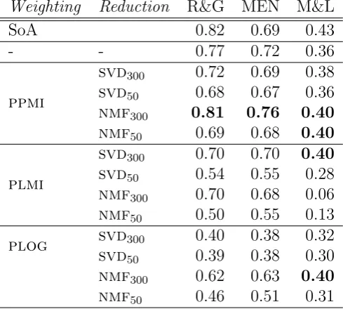
Based on the results of these quality evaluation experiments, reported in Ta-ble 2.1, both the full and pPMI-transformed semantic spaces obtain state-of-the-art results. The best performing semantic space across the board is the space in which the raw cooccurrence counts are transformed with pPMI and the full 1Of the 1,000 word pairs in the MEN test set, our semantic space covered 773 of these data
Weighting Reduction R&G MEN M&L
SoA 0.82 0.69 0.43
- - 0.77 0.72 0.36
ppmi
svd300 0.72 0.69 0.38
svd50 0.68 0.67 0.36
nmf300 0.81 0.76 0.40
nmf50 0.69 0.68 0.40
plmi
svd300 0.70 0.70 0.40
svd50 0.54 0.55 0.28
nmf300 0.70 0.68 0.06
nmf50 0.50 0.55 0.13
plog svd300 0.40 0.38 0.32 svd50 0.39 0.38 0.30
nmf300 0.62 0.63 0.40
nmf50 0.46 0.51 0.31
12K-by-10K space is reduced to 12K-by-300 with NMF.
2.2
Composition models
I focus on six composition functions proposed in recent literature with high per-formance in a number of semantic tasks. I first consider methods proposed by Mitchell & Lapata (2010) in which the model-generated vectors are simply ob-tained through component-wise operations on the constituent vectors. Given input vectors�uand�v, Mitchell & Lapata derive two simplified models from these general forms. The first of which is the simplified additive model (add), given by Equation 2.5, and can be extended to the weighted additive model (w.add) in which a composed vector is obtained as a weighted sum of the two component vectors, Equation 2.6, where α and β are scalars.
�c=�u+�v (2.5)
�c=α�u+β�v (2.6)
Next, a simplified multiplicative (mult) approach that reduces to component-wise multiplication, where the i-th component of the composed vector is given by: pi =uivi, generalized by Equation 2.7.
�c=�u⊙�v (2.7)
Mitchell & Lapata extend the multiplicative approach to a basis-independent composition which is based solely on the geometry of u and v, referred to here as the dilation method (dl):
�c= (�u·�u)�v+ (λ−1)(�u·�v)�u (2.8)
to emphasize the contribution of �u.
Mitchell & Lapata evaluate the simplified models on a wide range of tasks ranging from paraphrasing to statistical language modeling to predicting similar-ity intuitions. Both simple models fare quite well across tasks and alternative semantic representations, also when compared to more complex methods derived from the equations above. Given their overall simplicity, good performance and the fact that they have also been extensively tested in other studies (Baroni & Zamparelli, 2010; Erk & Pad´o, 2008; Guevara, 2010; Kintsch, 2001; Landauer & Dumais, 1997), I re-implement here the add, w.add, mult and dl models. In addition to finding that the mult, w.add and dl models perform best overall, Mitchell & Lapata (2010) observed that the dl models performed consistently well across all representations.
Mitchell & Lapata (as well as earlier researchers) do not exploit corpus evi-dence about the�cvectors that result from composition, despite the fact that it is straightforward (at least for short constructions) to extract direct distributional evidence about the composite items from the corpus (just collect co-occurrence information for the composite item from windows around the contexts in which it occurs). Here, I also consider the full extension of the additive model (f.add), presented in Guevara (2010) and Zanzottoet al.(2010), such that the component vectors are pre-multiplied by weight matrices before being added, Equation 2.9:
�c=W1�u+W2�v (2.9)
The main innovation of Guevara (2010), who focuses on adjective-noun combina-tions (AN), is to use the co-occurrence vectors of corpus-observed ANs to train a supervised composition model. Guevara adopts the full additive composition form from Equation (2.9) and he estimates theW1andW2weights (concatenated
ANs generated by his model than to those from the alternative approaches. The add model, on the other hand, is best in terms of shared neighbor count between corpus-extracted and model-generated ANs.
Finally, I consider the lexical function model (lfm), first introduced in Ba-roni & Zamparelli (2010), in which attributive adjectives are treated as functions from noun meanings to noun meanings. This is a standard approach in Montague semantics Thomason (1974), except noun meanings here are distributional vec-tors, not denotations, and adjectives are (linear) functions learned from a large corpus. In this model, composed vectors are generated by multiplying a function matrix U, representing the adjective at hand, with a component (noun) vector, Equation 2.10.
�c=U�v (2.10)
In Baroni & Zamparelli (2010), they show that the model significantly outper-forms other vector composition methods, including add, mult and f.add, in the task of approximating the correct vectors for previously unseen (but corpus-attested) ANs.
2.2.1
Composition model estimation
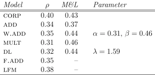
Parameters forw.add,dl,f.addandlfmwere estimated following the strategy proposed by Guevara (2010) and Baroni & Zamparelli (2010), recently extended to all composition models by Dinu et al. (2013b). Specifically, I learn parameter values that optimize the mapping from the noun to the AN as seen in exam-ples of corpus-extracted N-AN vector pairs, using least-squares methods for all models except lfm. All parameter estimations and phrase compositions were im-plemented using the DISSECT toolkit (Dinuet al., 2013a, http://clic.cimec. unitn.it/composes/toolkit), with a training set of 74,767 corpus-extracted N-AN vector pairs, ranging from 100 to over 1K items across the 663 adjec-tives. Table 2.2 reports the results attained by our model implementations on the Mitchell & Lapata AN similarity data set.
Model ρ M&L Parameter corp 0.40 0.43
add 0.34 0.37
w.add 0.35 0.44 α= 0.31, β = 0.46 mult 0.31 0.46
dl 0.32 0.44 λ= 1.59
f.add 0.35 –
lfm 0.38 –
Table 2.2: Composed space quality evaluation. Correlation scores (Spear-man’s ρ, all significant at p<0.001) between cosines of corpus-extracted (corp) or model-generated AN vectors and phrase similarity ratings collected in Mitchell & Lapata (2010), as well as best reported results from Mitchell & Lapata (M&L).
noun. The linear equation coefficients were estimated separately for each adjective using Ridge regression with generalized cross-validation (GCV) to automatically choose the optimal Ridge parameter for each adjective (Golub et al., 1979). For each adjective, the training N-AN vector pairs chosen were those available in the training set.
Degrees of adjective modification
in distributional semantics
3.1
Introduction
One of the most appealing aspects of so-called distributional semantic models (see Turney & Pantel (2010) for a recent overview) is that they afford some hope for a non-trivial, computationally tractable treatment of the context dependence of lexical meaning that might also approximate in interesting ways the psychological representation of that meaning (Andrewset al., 2009). However, in order to have a complete theory of natural language meaning, these models must be supplied with or connected to a compositional semantics; otherwise, we will have no account of the recursive potential that natural language affords for the construction of novel complex contents.
In the last 4-5 years, researchers have begun to introduce compositional oper-ations on distributional semantic representoper-ations, for instance to combine verbs with their arguments or adjectives with nouns (Baroni & Zamparelli, 2010; Erk & Pad´o, 2008; Grefenstette & Sadrzadeh, 2011b; Mitchell & Lapata, 2010; Socher et al., 2011)1. Although the proposed operations have shown varying degrees of
it remains unclear to what extent they can account for the full range of meaning composition phenomena found in natural language. Higher-order modification (that is, modification that cannot obviously be modeled as property intersection, in contrast to first-order modification, which can) presents one such challenge, as we will detail in the next section.
The goal of this chapter is twofold. First, we examine how the properties of different types of adjectival modifiers, both in isolation and in combination with nouns, are represented in distributional models. We take as a case study three groups of adjectives: 1) color terms used to ascribe true color properties (referred to here as intersective color terms), as prototypical representative of first-order modifiers; 2) color terms used to ascribe properties other than simple color (here, subsectivecolor terms), as representatives of expressions that could in principle be given a well-motivated first-order or higher-order analysis; and 3)
intensionaladjectives (e.g. former), as representative of modifiers that arguably require a higher-order analysis. Formal semantic models tend to group the second and third groups together, despite the existence of some natural language data that questions this grouping. However, our results show that all three types of modifiers behave differently from each other, suggesting that their semantic treatment needs to be differentiated.
Second, we test how five different composition functions that have been pro-posed in recent literature fare in predicting the attested properties of nominals modified by each type of adjective. The model by Baroni & Zamparelli (2010) emerges as a suitable model of adjectival composition, while multiplication and addition shed mixed results.
3.2
The semantics of adjectival modification
Accounting for inference in language is an important concern of semantic the-ory. Perhaps for this reason, within the formal semantics tradition the most influential classification of adjectives is based on the inferences they license (see Parsons (1970) and Kamp (1975) for early discussion). We very briefly review this classification here.
First, so called intersective adjectives, such as (the literally used) white in white dress, yield the inference that both the property contributed by the adjective and that contributed by the noun hold of the individual described; in other words, a white dress is white and is a dress. The semantics for such modifiers is easily characterized in terms of the intersection of two first-order properties, that is, properties that can be ascribed to individuals.
On the other extreme, intensional adjectives, such as former or alleged in former/alleged criminal, do not license the inference that either of the properties holds of the individual to which the modified nominal is ascribed. Indeed, such adjectives cannot be used as predicates at all:
(1) ??The criminal was former/alleged.
The infelicity of (1) is generally attributed to the fact that these adjectives do not describe individuals directly but rather effect more complex operations on the meaning of the modified noun. It is for this reason that these adjectives can be considered higher-order modifiers: they behave as properties of proper-ties. Though rather abstract, the higher-order analysis is straightforwardly im-plementable in formal semantic models and captures a range of linguistic facts successfully.
color in question may or may not match the color identified by the adjective on the intersective use (see G¨ardenfors (2000) and Kennedy & McNally (2010) for discussion and analysis). The effect of the adjective, rather than to identify a value for an incidental color attribute of an object, is often to characterize a subclass of the class described by the noun (white wine is a kind of wine, brown rice a kind of rice, etc.).
This use of color terms can be modeled by property intersection in formal semantic models only if the term is previously disambiguated or allowed to depend on context for its precise denotation. However, it is easily modeled if the adjective denotes a (higher-order) function from properties (e.g. that denoted by wine) to properties (that denoted by white wine), since the output of the function denoted by the color term can be made to depend on the input it receives from the noun meaning. Nonetheless, there is ample evidence in natural language that a first-order analysis of the subsective color terms would be preferable, as they share more features with predicative adjectives such as happy than they do with adjectives such as former.
The trio of intersective color terms, subsective color terms, and intensional adjectives provides fertile ground for exploring the different composition functions that have been proposed for distributional semantic representations. Most of these functions start from the assumption that composition takes pairs of vectors (e.g. a verb vector and a noun vector) and returns another vector (e.g. a vector for the verb with the noun as its complement), usually by some version of vector addition or multiplication (Erk & Pad´o, 2008; Grefenstette & Sadrzadeh, 2011b; Mitchell & Lapata, 2010). Such functions, insofar as they yield representations which strengthen distributional features shared by the component vectors, would be expected to model intersective modification.
Additive and multiplicative functions might also be expected to handle sub-sective modification with some success because these operations provide a natural account for how polysemy is resolved in meaning composition. Thus, the vector that results from adding or multiplying the vector for white with that for dress should differ in crucial features from the one that results from combining the same vector for white with that for wine. For example, depending on the details of the algorithm used, we should find the frequencies of words such as snow or milky weakened and words like straw oryellow strengthened in combination withwine, insofar as the former words are less likely than the latter to occur in contexts where white describes wine than in those where it describes dresses. In contrast, it is not immediately obvious how these operations would fare with intensional adjectives such asformer. In particular, it is not clear what specific distributional features of the adjective would capture the effect that the adjective has on the meaning of the resulting modified nominal.
Interestingly, recent approaches to the semantic composition of adjectives with nouns such as Baroni & Zamparelli (2010) and Guevara (2010) draw on the classical analysis of adjectives within the Montagovian tradition of formal semantic theory (Montague, 1974), on which they are treated as higher order predicates, and model adjectives as matrices of weights that are applied to noun vectors. On such models, the distributional properties of observed occurrences of adjective-noun pairs are used to induce the effect of adjectives on nouns. Insofar as it is grounded in the intuition that adjective meanings should be modeled as mappings from noun meanings to adjective-noun meanings, the matrix analysis might be expected to perform better than additive or multiplicative models for adjective-noun combinations when there is evidence that the adjective denotes only a higher-order property. There is also no a priori reason to think that it would fare more poorly at modeling the intersective and subsective adjectives than would additive or multiplicative analyses, given its generality.
3.3
Methodology
3.3.1
Evaluation material
We built two datasets of adjective-noun phrases for the present research, one with color terms and one with intensional adjectives.1
Color terms. This dataset is populated with a randomly selected set of adjective-noun pairs from the space presented above. From the 11 colors in the basic set proposed by Berlin & Kay (1969), we cover 7 (black,blue,brown,green,red,white, and yellow), since the remaining (grey, orange, pink, and purple) are not in the 700 most frequent set of adjectives in the corpora used. From an original set of 412 ANs, 43 were manually removed because of suspected parsing errors (e.g. white photograph, forblack and white photograph) or because the head noun was semantically transparent (white variety). The remaining 369 ANs were tagged independently by the second and fourth authors of Boleda et al. (2012), both native English speaker linguists, as intersective (e.g. white towel), subsective
(e.g. white wine), oridiomatic, i.e. compositionally non-transparent (e.g. black hole). They were allowed the assignment of at most two labels in case of poly-semy, for instance for black staff for the person vs. physical object senses of the noun oryellow skin for the race vs. literally painted interpretations of the AN. In this chapter, only the first label (most frequent interpretation, according to the judges) has been used. Theκcoefficient of the annotation on the three categories (first interpretation only) was 0.87 (conf. int. 0.82-0.92, according to Fleiss et al. (1969)), observed agreement 0.96.2 There were too few instances of idioms (17)
for a quantitative analysis of the sort presented here, so these are collapsed with the subsective class in what follows.3 The dataset as used here consists of 239
intersective and 130 subsective ANs.
1Available at http://dl.dropbox.com/u/513347/resources/data-emnlp2012.zip. See
Bruni et al.(2012) for an analysis of the color term dataset from a multimodal perspective. 2Code for the computation of inter-annotator agreement by Stefan Evert, available athttp:
//www.collocations.de/temp/kappa_example.zip.
Intensional adjectives. The intensional dataset contains all ANs in the se-mantic space with a pre-selected list of 10 intensional adjectives, manually pruned by one of the authors of Boleda et al.(2012) to eliminate erroneous examples and to ensure that the adjective was being intensionally used. Examples of the ANs eliminated on these grounds include past twelve (cp. accepted past president), former girl (probablyformer girl friend or similar), false rumor (which is a real rumor that is false, vs. e.g. false floor, which is not a real floor), or theoretical work (which is real work related to a theory, vs. e.g. theoretical speed, which is a speed that should have been reached in theory). Other AN pairs were excluded on the grounds that the noun was excessively vague (e.g. past one) or because the AN formed a fixed expression (e.g. former USSR). The final dataset contained 1,200 ANs, distributed as follows: former (300 examples), possible (244), future (243), potential (183), past (87), false (44), apparent (39), artificial (36), likely (18), theoretical (6).1 Table 3.1 contains examples of each type of AN we are
considering.
Intersective Subsective Intensional white towel white wine artificial leg black sack black athlete former bassist green coat green politics likely suspect red disc red ant possible delay blue square blue state theoretical limit
Table 3.1: Example ANs in the datasets.
3.4
Results
3.4.1
Corpus-extracted vectors
We began by exploring the empirically corpus-extracted vectors for the ad-jectives (A), nouns (N), and adjective-noun phrases (AN) in the datasets, as they are represented in the semantic space. Note that we are working with the AN vec-tors directly harvested from the corpora (that is, based on the co-occurrence of, say, the phrase white towel with each of the 10K words in the space dimensions), without doing any composition. AN vectors obtained by composition will be examined in the following section. Though corpus-extracted AN vectors should not be regarded as a gold standard in the sense of, for instance, Machine Learn-ing approaches, because they are typically sparse1 and thus the vectors of their
component adjective and noun will be richer, they are still useful for exploration and as a comparison point for the composition operations (Baroni & Lenci, 2010; Guevara, 2010).
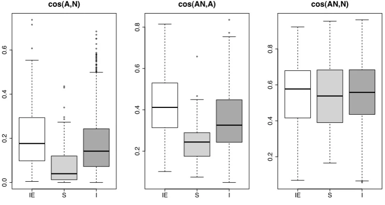
Figure 3.1 shows the distribution of the cosines between A, N, and AN vectors with intersective uses of color terms (IE, white box), subsective uses of color terms (S, lighter gray box), and intensional adjectives (I, darker gray box).
In general, the similarity of the A and N vectors is quite low (cosine < 0.2, left graph of Figure 1), and much lower than the similarities between both the AN and A vectors and the AN and N vectors. This is not surprising, given that adjectives and nouns describe rather different sorts of things.
We find significant differences between the three types of adjectives in the similarity between AN and A vectors (middle graph of Figure 3.1). The adjective and adjective-noun phrase vectors are nearer for intersective uses than for sub-sective uses of color terms, a pattern that parallels the difference in the distance between component A and N vectors. Since intersective uses correspond to the prototypical use of color terms (awhite dress is the color white, whilewhite wine is not), the greater similarity for the intersective cases is unsurprising – it sug-gests that in the case of subsective adjectival modifiers, the noun “pulls” the AN 1The frequency of the adjectives in the datasets range from 3.5K to 3.7M, with a median
● ● ● ● ● ● ● ● ● ● ● ● ● ● ● ● ● ● ● ● ● ● ● ● ● ● ● ● ● ● ● ● ● ● ● ● ● ●
IE S I
0.0 0.2 0.4 0.6 cos(A,N) ● ● ● ●
IE S I
0.2 0.4 0.6 0.8 cos(AN,A) ● ●
IE S I
0.2
0.4
0.6
0.8
cos(AN,N)
Figure 3.1: Cosine distance distribution in the different types of AN. We report the cosines between the component adjective and noun vectors (cos(A,N)), be-tween the corpus-extracted AN and adjective vectors (cos(AN,A)), and bebe-tween the corpus-extracted AN and noun vectors (cos(AN,N)). Each chart contains three boxplots with the distribution of the cosine scores (y-axis) for the intersec-tive (IE), subsecintersec-tive (S) and intensional (I) types of ANs. The boxplots represent the value distribution of the cosine between two vectors. The horizontal lines in the rectangles represent the first quartile, median, and third quartile. Larger rectangles correspond to a more spread distribution, and their (a)symmetry mir-rors the (a)symmetry of the distribution. The lines above and below the rectangle stretch to the minimum and maximum values, at most 1.5 times the length of the rectangle. Values outside this range (outliers) are represented as points.
further away from the adjective than happens with the cases of intersective mod-ification. This is compatible with the intuition (manifest in the formal semantics tradition in the treatment of subsective adjectives as higher-order rather than first-order, intersective modifiers) that the adjective’s effect on the AN in cases of subsective modification depends heavily on the interpretation of the noun with which the adjective combines, whereas that is less the case when the adjective is used intersectively.
with both intersective and subsective color terms. We hypothesize that the results for the intensional adjectives are due to the fact that they cannot plausibly be modeled as first order attributes (i.e. beingpotential orapparent is not a property in the same sense that beingwhite oryellow is) and thus typically do not restrict the nominal description per se, but rather provide information about whether or when the nominal description applies. The result is that intensional adjectives should be even weaker than subsectively used adjectives, in comparison with the nouns with which they combine, in their ability to “pull” the AN vector in their direction. Note, incidentally, that an alternative explanation, namely that the effect mentioned could be due to the fact that most nouns in the intensional dataset are abstract and that adjectives modifying abstract nouns might tend to be further away from their nouns altogether, is ruled out by the comparison between the A and N vectors: the A-N cosines of the intensional and intersective ANs are similar. We thus conclude that here we see an effect of the type of modification involved.
An examination of the average distances among the nearest neighbors of the intensional and of the color adjectives in the distributional space supports our hypothesized account of their contrasting behaviors. We predict that the nearest neighbors are more dispersed for adjectives that cannot be modeled as first-order properties (i.e., intensional adjectives), than for those that can (here, the color terms). We find that the average cosine distance among the nearest ten neighbors of the intensional adjectives is 0.74 with a standard deviation of 0.13, which is significantly lower (t-test,p<0.001) than the average similarity among the nearest neighbors of the color adjectives, 0.96 with astandard deviation of 0.04.
Finally, with respect to the distances between the adjective-noun and head noun vectors (right graph of Figure 1), there is no significant difference for the intersective vs. subsective color terms. This can be explained by the fact that both kinds of modifiers are subsective, that is, the fact that a white dress is a dress and that white wine is wine.
by the fact that intensional adjectives do not restrict the descriptive content of the noun they modify, in contrast to both the intersective and subsective color ANs. Restriction of the nominal description may lead to significantly restricted distributions (e.g. the phrase red button may appear in distinctively different contexts than does button; similarly for green politics and politics), while we do not expect the contexts in which former bassist and bassist appear to diverge in a qualitatively different way because the basic nominal descriptions are identical, though further research will be necessary to confirm these explanations.
Finally, note that, contrary to predictions from some approaches in formal semantics, subsective color ANs and intensional ANs do not pattern together: subsective ANs are closer to their component As, and intensional ANs closer to their component Ns. This unexpected behavior underscores the fact highlighted in the previous paragraph: that the distributional properties of modified expressions are more sensitive to whether the modification restricts the nominal description than to whether the modifier is intersective in the strictest sense of term.
We now discuss the extent to which the different composition functions ac-count for these patterns.
3.4.2
Model-generated vectors
Since intersective modification is the point of comparison for both subsective and intensional modification, we first discuss the model-generated vectors for the intersective vs. subsective uses of color terms, and then turn to intersective vs. intensional modification.
Intersective and subsective modification with color terms. To adequately model the differences between intersective and subsective modification observed in the previous section, a successful composition function should not only gener-ate AN vectors that approximgener-ate the corpus-extracted AN vectors; it should also yield a significantly smaller distance between the adjective and AN vectors for intersectively used adjectives, whereas it should yield no significant difference for the distances between the noun and AN vectors.
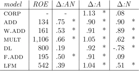
(corp) and the composition functions discussed in Section 2.2. The median rank of corpus-observed equivalent (ROE) is provided as a general measure of the quality of the composition function. It is computed by finding the cosine between the model-generated AN vectors and all rows in the semantic space and then determining the rank in which the corpus-extracted ANs are found.1
The remaining columns report the differences in standardized (z-score) cosines between the vector built with each of the composition functions and the corpus-extracted AN, A, and N vectors. A positive value means that the cosines for intersective uses are higher, while a negative value means that the cosines for subsective uses are higher. The first row (corp) contains a numerical summary of the tendencies for corpus-extracted ANs explained in the previous section. This is the behavior that we expect to model.
model ROE ∆:AN ∆:A ∆:N
corp - - 1.13 * .08
add 134 .75 * .90 * .90 *
w.add 161 .53 * .91 * .89 * mult 1,106 .66 * 1.05 * .62 *
dl 800 .19 .92 * -.78 *
f.add 195 .50 * .91 * .09
lfm 542 .39 1.04 * .51 *
Table 3.2: Intersective vs. subsective uses of color terms. The first column reports the rank of the corpus-observed equivalent (ROE), the rest report the differences (∆) betwen the intersective and subsective uses of color terms when comparing the model-generated AN with the corpus-extracted vectors for: AN, adjective (A), noun (N). See text for details. Significances according to a t-test: * for p<0.001.
One composition function comes close to modeling the corpus-observed be-havior: f.add. In this case, we find that the function yields higher similarities for AN-A for the intersective than for the subsective uses of color terms, and a very slight difference for the distance to the head noun. The mult and lfm models approximate the corpus-observed behavior best with respect to the distance from 1The ROE is provided as a general guide; however, recall that the ROE was taken into
to the component adjective. Although they are unable to capture the observed, and expected, effect in the distance from the head noun, there is an asymmetry that we would expect between these measure in both composition models. The addandw.addfunctions perform very well in terms of ROE (median 134). This suggests that, for adjectival modification, providing a vector that is in the mid-dle of the two component vectors (which is what normalized addition does), or slightly skewed towards the head in the case of w.add, is a reasonable approxi-mation of the corpus-extracted vectors. However, precisely because the resulting vector is in the middle of the two component vectors, these functions cannot ac-count for the asymmetries in the distances found in the corpus-observed data. One might expect that a non-normalized version of add could not account for these effects because the adjective vector, being much longer (as color terms are very frequent), would totally dominate the AN, resulting in no difference across uses when comparing to the adjective or to the noun.
The dl model shows a strange pattern, as it yields a strongly significant negative difference in the AN-N distance. This is likely a result of the intuitive choice of the adjective vector as �u and the noun vector as �v in composition (see Equation 2.8). A post-hoc analysis showed that if we were to reverse the assignment (i.e., the adjective vector as�v and the noun vector as�u), we find that the results are quantitatively identical, however reversed, i.e., ∆:A= −.78 and ∆:N= .92. Themult model is by far the worst function in terms of ROE, which can be attributed to the sparsity of the model-generated vectors after point-wise multiplication of NFM-reduced component vectors.
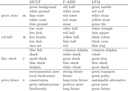
MULT F.ADD LFM
green stone ie
green background old wall green marble white ground white stone red roof
blue wave red tower white stone
white cross red stone yellow stone
blue ground stone green tile
red ball ie
low cross other ball white triangle
free kick red ball blue square
free header yellow ball black colour
low shot blue ball black cross
own net red blue ring
blue shark s
blue fish common dolphin common dolphin
shark white shark whale
small shark great shark green frog
blue shark blue shark blue shark
dolphin white whale great shark
green future s
environmental asset strong future green transport local biodiversity future green policy
conservation long-term future sustainable alternative green infrastructure positive news green issue
biodiversity long future green future
Table 3.3: Examples of nearest neighbors for color terms according to the three composition models in intersective (IE) vs. subsective (S) color terms: mult, f.add and lfm.
and lfm functions. In the case of lfm, the weights for each adjective matrix are estimated in relation to the noun vectors with which the adjective combines, on the one hand, and the related corpus-extracted AN vectors, on the other; thus, the basic lexical representation of the adjective is inherently reflective of the distributions of the ANs in which it appears in a way that is not the case for the adjective representations used in the other composition models. And indeed, dl andlfmare the only functions that show no difference in difficulty (distance) between the model-generated and corpus-extracted AN vectors for intersective vs. subsective ANs.
the semantics of adjective composition in this case to a larger extent than both f.addandmult. Consider the difference in nearest neighbors of intersective and subsective color terms in Table 3.3.
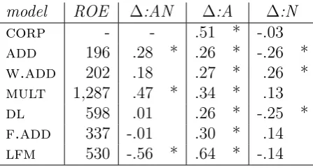
Intensional modification. Table 3.4 contains the results of the composition functions comparing the behavior of intersective color ANs and intensional ANs. The tendencies in the ROE are as in Table 3.2, so we will not comment on them further (note the very poor performance of mult, though). As noted above, we expect more difficulty in modeling intensional modification vs. other kinds of modification, however this is verified in the results for only the add and mult models (cf. the positive values in second column), and only slightly for w.add. While we find that thelfmmodel is able to approximate corpus-observed vectors for intensional modification easier than for intersective uses of color terms. This points to a qualitative difference between subsective and intensional adjectives that could be evidence for a first-order analysis of subsective color terms. (See Boleda et al. (2013) for an extended study on detecting intensional modification using compositional distributional semantics.)
model ROE ∆:AN ∆:A ∆:N
corp - - .51 * -.03
add 196 .28 * .26 * -.26 *
w.add 202 .18 .27 * .26 * mult 1,287 .47 * .34 * .13
dl 598 .01 .26 * -.25 *
f.add 337 -.01 .30 * .14
lfm 530 -.56 * .64 * -.14
Table 3.4: Intersective vs. intensional ANs. Information as in Table 3.2.
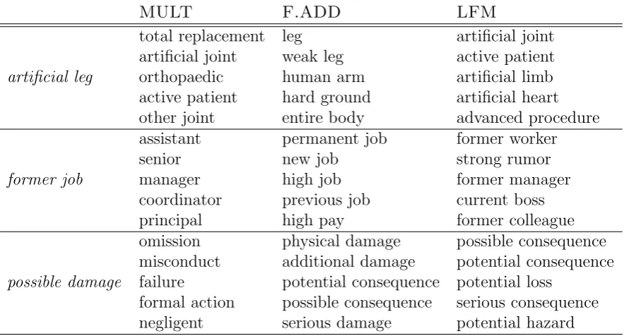
A good composition function should provide a large positive difference when comparing the AN to the A, and a small negative difference (because the effect is not significant in the corpus-observed data) when comparing the AN to the N. The functions that best match the corpus-observed data are again lfm, f.add and mult. Addand dl show the predicted pattern, but to a much lesser degree (cf. smaller differences in column ∆:A).
MULT F.ADD LFM
artificial leg
total replacement leg artificial joint artificial joint weak leg active patient
orthopaedic human arm artificial limb
active patient hard ground artificial heart other joint entire body advanced procedure
former job
assistant permanent job former worker
senior new job strong rumor
manager high job former manager
coordinator previous job current boss
principal high pay former colleague
possible damage
omission physical damage possible consequence misconduct additional damage potential consequence failure potential consequence potential loss
formal action possible consequence serious consequence negligent serious damage potential hazard
Table 3.5: Examples of nearest neighbors for intensional terms according to the three composition models: mult, f.add and lfm.
with intensional adjectives, as seen in Table 3.5..
3.5
Discussion
The present research provides evidence for treating adjectives as matrices or func-tions, rather than vectors, although simple operations on vectors such asaddand w.add (for their excellent approximation to observed vectors) still account for some aspects of adjectival modification. The mult model, in contrast, struggles to approximate adjectival modification (as seen in the poor ROE scores) likely due to the sparse, or even zero, vectors that result after point-wise multiplication of NMF-reduced component vectors. This is a serious drawback of the mult model.
2.5K ANs, while our semantic space contains more than 170K ANs. However, the linguistic literature and the present results suggest that it might be useful to try a compromise between lfmand f.add, training one matrix for each subclass of adjectives under analysis.
Capturing semantic deviance
4.1
Introduction
A prominent approach for representing the meaning of a word in Natural Lan-guage Processing (NLP) is to treat it as a numerical vector that codes the pattern of co-occurrence of that word with other expressions in a large corpus of language (Sahlgren, 2006; Turney & Pantel, 2010): the meaning of the word painting, for instance, could be characterized in terms of its proximity with artist, museum, colorful, abstract, etc. This approach to semantics (sometimes called distribu-tional semantics) naturally captures collocations, scales well to large lexicons and does not require words to be manually disambiguated (Sch¨utze, 1997). Until recently, however, this method had been almost exclusively limited to the level of content words (nouns, adjectives, verbs), and had not directly addressed the problem of compositionality (Frege, 1892; Partee, 2004), the crucial property of natural language which allows speakers to derive the meaning of a complex lin-guistic constituent from the meaning of its immediate syntactic subconstituents. Together with a generative syntactic component (Chomsky, 1957), this principle is responsible for the productivity of natural language, which allows speakers to produce and understand sentences they have never encountered before.
vec-tor space (Baroni & Zamparelli, 2010; Blacoe & Lapata, 2012; Grefenstette & Sadrzadeh, 2011a; Guevara, 2010; Mitchell & Lapata, 2010; Socher et al., 2012). All these approaches manage to construct distributional semantics representa-tions for novel phrases, starting from the corpus-derived vectors for their lexical constituents. Since their output is naturally graded, these methods also promise to address the fact that compositionality is a matter of degree (Nunberg et al., 1994), ranging from fully compositional cases, as in those attributive adjective-noun phrases whose meaning is the intersection of the meaning of the adjective-noun and adjective (e.g. rented car, wooden spoon), to syntactically fixed expressions such as take advantage, cut a deal, where the meaning of some of their subparts can still be recognized in the final meaning, to idioms and multi-word expressions (kick the bucket, red herring,by and large), whose meaning cannot be distributed at all across their constituents. Despite these latter cases, language is still largely compositional, providing an open space for speakers to create novel but under-standable complex linguistic expressions.
Yet, linguistic creativity has its limits: as native speakers we have the clear intuition that not all of the infinitely many possible syntactically well-formed strings are equally semantically acceptable. Chomsky’s classic example in (1) was devised precisely to show that syntax and semantics can diverge.
(1) Colorless green ideas sleep furiously
Our knowledge of compositionality tells us that here the lexical semantics of the words colorless, green and ideas did not combine properly. The result is a semantically deviant phrase which cannot be used in ‘normal’ contexts (e.g. non-metalinguistic ones—see below for some qualifications), and therefore will not be found in corpora, not even very large ones, since corpora largely document actual, normal language use.
linguistics from the generative linguistic community was precisely that (crude) statistical approaches could not distinguish between these various possibilities (cf. Chomsky’s famous remark that “I live in Dayton, Ohio” is not less grammatical, nor indeed, less meaningful, that “I live in New York”, despite being far less frequent).
In this study we show that it is possible to use compositional distributional methods to distinguish the unattestedness due to nonsensicality from all the other cases, in the domain of simple noun phrases. Specifically, we show that distri-butional measures such as vector length, neighbor density and cosine distance can reliably predict the extent to which a novel adjective-noun combination—one never found in a corpus and never seen by the system in the training phase— makes sense. Moreover, we show that these distributional measures improve over shallow, word-based measures like word length or word frequency. Finally, we show that this result holds across a variety of compositional methods proposed in the literature, though some are of course better then others in various subtasks.
To put the problem in context, consider the difference between two adjective-noun phrases in (2) which are not attested in a large corpus of English.
(2) a. grooved tangerine b. residential steak
Although it may be the case that you have never considered that a tangerine could have grooves, such an object is easy to imagine and it can be understood in out-of-the-blue contexts. On the other hand, residential steak describes an object that is quite hard to imagine. In what sense can a steak be residential? Perhaps in none, perhaps in too many: in the context of a man who always and only eats steak when he is in his residence, his usual residential steak makes sense. Notice, however, that now the adjective is used only as a proxy for a larger description (eaten when in residence). Out of the blue,residential steak is semantically very odd, grooved tangerine is not (though it might be factually strange, whence its absence). In truly semantically deviant cases, different speakers would probably not even agree on how to paraphrase the expressions, if given in isolation.
what it means for a linguistic expression to be “nonsensical”, nor a clear relation between this notion and that of being unattested in a corpus: semantic deviance remains a difficult and understudied phenomenon. In formal denotation-based semantics, for instance, a ‘meaningless sentence’ could perhaps be characterized as one which is false in any imaginable situation (say, in any epistemically accessible possible world). However, this approach would still be unable to determine the degree or even the motivation for the deviance, and could not predict when a novel string will be nonsensical. Moreover, there are many necessarily false expressions such as (3) which do not feel nonsensical, but simply false.
(3) 17 is not a prime
Thus, the task of distinguishing between unattested but acceptable and unat-tested but semantically deviant linguistic expressions is not only a way to address a criticism about the limits of corpus linguistics, but also an interesting linguistic task, whose solution could have an impact on the theoretical and com-putational linguistic community as a whole, and shape our future treatments of semantic deviance.
com-positional distributional semantics. Finally, we asses the effect of a number of variables in the ability to model the intuitions of semantic acceptability for novel phrases, on the basis of the acceptability judgments we collected. Since, to our knowledge, this is the first attempt to automatically model semantic acceptabil-ity computationally, we did not know a priori which features could be best for the task. Therefore, we used a variety or metrics, some taken from the cognitive and psycholinguistic literature on lexical processing and in particular compound processing, others designed by us and based on the distributional representation we are using. Evaluating the effectiveness of these measures, we show that dis-tributional semantics techniques go beyond semantically shallow wordform-based measures previously tested in psycholinguistic studies.
The unsupervised method we introduce for measuring and estimating the semantic deviance of phrases can be applied to a number of NLP tasks, such as metaphor analysis, the collection of better estimates for language modeling and a measure of plausibility in machine translation tasks.
Outline This section is structured as follows. Section 4.4.1 describes the design of the experiments discussed in this study, including the datasets used and the parameter-tuning phase for the composition methods. The measures we tested are described in Section 4.4.2, and our approach to data analysis is laid out in Section 4.4.2. We present the results of our experiments in Section 4.4.3 in three parts: (i) the ability of word-based measures to model the acceptability of novel AN phrases (our baseline); (ii) the measures extracted from estimated distributional representations of ANs which improve the ability to model semantic acceptability; and (iii) a detailed analysis of the performances of each composition function. Finally, Section 4.4.4 contains a discussion of the conclusions drawn from this study, as well as a number of issues that we would like to address in future research.
4.2
Related work
computa-tional linguistics, the possibility of detecting semantic deviance has been seen as a prerequisite to access metaphorical/non-literal semantic interpretations (Fass & Wilks, 1983; Zhou et al., 2007). In psycholinguistics, it has been part of a wide debate on the point at which context can make us perceive a ‘literal’ vs. a ‘figurative’ meaning (Giora, 2002). In theoretical generative linguistics, the issue is part of an ongoing discussion on the boundaries between syntax and semantics.
(4) Colorless gree