METHODOLOGY
A computational approach for the
functional classification of the epigenome
Francesco Gandolfi
1*and Anna Tramontano
1,2Abstract
Background: In the last decade, advanced functional genomics approaches and deep sequencing have allowed large-scale mapping of histone modifications and other epigenetic marks, highlighting functional relationships between chromatin organization and genome function. Here, we propose a novel approach to explore functional interactions between different epigenetic modifications and extract combinatorial profiles that can be used to anno-tate the chromatin in a finite number of functional classes. Our method is based on non-negative matrix factorization (NMF), an unsupervised learning technique originally employed to decompose high-dimensional data in a reduced number of meaningful patterns. We applied the NMF algorithm to a set of different epigenetic marks, consisting of ChIP-seq assays for multiple histone modifications, Pol II binding and chromatin accessibility assays from human H1 cells.
Results: We identified a number of chromatin profiles that contain functional information and are biologically inter-pretable. We also observe that epigenetic profiles are characterized by specific genomic contexts and show signifi-cant association with distinct genomic features. Moreover, analysis of RNA-seq data reveals that distinct chromatin signatures correlate with the level of gene expression.
Conclusions: Overall, our study highlights the utility of NMF in studying functional relationships between different epigenetic modifications and may provide new biological insights for the interpretation of the chromatin dynamics.
Keywords: Chromatin profiles, Epigenetic mark combinations, NMF
© The Author(s) 2017. This article is distributed under the terms of the Creative Commons Attribution 4.0 International License (http://creativecommons.org/licenses/by/4.0/), which permits unrestricted use, distribution, and reproduction in any medium, provided you give appropriate credit to the original author(s) and the source, provide a link to the Creative Commons license, and indicate if changes were made. The Creative Commons Public Domain Dedication waiver (http://creativecommons.org/ publicdomain/zero/1.0/) applies to the data made available in this article, unless otherwise stated.
Background
In eukaryotes, DNA is wrapped and packaged in nucle-osomes, which represent the fundamental unit of the chromatin. Each nucleosome consists of an octamer of four different histone proteins: H2A, H2B, H3 and H4. These subunits undergo several types of chemical modi-fications on their N-terminal chain, including phospho-rylation, methylation and acetylation. It has been shown that posttranslational modifications of histone proteins can modulate the structural and functional properties of the chromatin and may be associated with transcriptional activation or repression [1], suggesting that they play a key role in determining the genetic profile of distinct types of cells. However, understanding which molecular
mechanisms and epigenetic changes are involved in the control of the gene expression still remains a challenge [2, 3]. Moreover, experimental evidences clearly suggest that many epigenetic modifications do not act as isolated signals along the DNA but tend to co-occur in a range of combinatorial patterns that can demarcate distinct func-tional elements on the genome [4].
In the last decade, advanced functional genomic tech-niques and NGS sequencing (ChIP-seq, DNase-seq) have allowed large-scale mapping of histone modifications and other epigenetic marks, highlighting functional relation-ships between chromatin states and transcriptional activ-ity. As genome-wide approaches became popular, broad datasets of different type of epigenetic data started being collected in public databases. Nowadays, two major con-sortia, the ENCODE (The ENCyclopedia Of Dna Ele-ments) project [5] and the NIH Roadmap Epigenomics [6], are acquiring data on multiple types of genomic assays,
Open Access
*Correspondence: [email protected]
1 Department of Physics, Sapienza University of Rome, Piazzale Aldo Moro
2, 00185 Rome, Italy
including DNA methylation, histone modifications, chro-matin accessibility and TF binding profiles for specific tissues/cell lines providing powerful resources to investi-gate several aspects of the chromatin organization. With the expanding amount of chromatin data publicly avail-able, an increasing interest in developing computational methods able to integrate different types of epigenetic signals and identify biologically meaningful combinations of chromatin marks has emerged. Most of the proposed algorithms are based on unsupervised classification tech-niques aimed at identifying recurrent patterns of chro-matin modifications from a given set of chrochro-matin marks. One of the early methods, ChromaSig [7], attempts to identify commonly occurring chromatin signatures in a pre-defined set of signal-enriched loci using a pattern-finding algorithm and unsupervised clustering techniques. The approach was initially applied to nine different epige-netic marks on 1% of the human genome [8] and identified epigenetic signatures that strongly correlate with distinct types of promoters and enhancers. However, the proce-dure is restricted to all regions with high levels of epige-netic modifications and does not allow a full exploration of all mark co-occurrence. Other popular tools such as ChromHMM [9], Segway [10] and EpicSeg [11] partially overcome this limit providing integrative models to extract combinatorial patterns from multiple genomic experi-ments. All these algorithms rely on the relatively new concept of chromatin segmentation. In this approach, a genome is fully partitioned in non-overlapping segments of a fixed length and raw reads are assigned to segments (or bins) generating a count-based distribution for a given functional genomic assay. The process is repeated for each epigenetic mark generating genome-wide normalized sig-nals of multiple genomic tracks along the chromosomic coordinate. Epigenetic signals are then processed through an unsupervised learning algorithm to infer the most probable chromatin state in each interval (i.e., a recurrent pattern of a given combination of marks). ChromHMM and EpicSeg are very similar and employ multivariate hid-den Markov model to reconstruct the sequence of hidhid-den states given a vector of observed frequencies (epigenetic marks). In ChromHMM, read count distributions are first converted in binned data tracks to reflect the presence/ absence of a particular mark in each segment according to a sample-specific probabilistic threshold. This HMM approach is computationally efficient, but does not allow a full-scale analysis of the chromatin modification levels and therefore loss of quantitative information is unavoid-able. In their work, Mammana et al. [11] propose a slightly different version of the HMM segmentation algorithm where raw read counts are directly used as observation variables instead of binary values. Observed counts for each epigenetic mark in each state are then modeled by
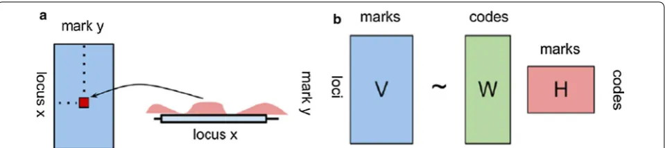
a negative multinomial distribution to take into account overdispersion of the data. Segway is conceptually close to ChromHMM and EpicSeg, but employs a dynamic Bayes-ian networks model to infer the most probable sequence of chromatin states at 1-bp resolution. Despite their appli-cability, these segmentation algorithms still suffer from a number of practical limitations that make chromatin state analysis not trivial. First, in most of these methods the number of chromatin states is arbitrarily fixed a priori to allow biological interpretation of the results. This solution is convenient in practical terms but does not allow estima-tion of the optimal number of states for a given set of epi-genetic marks. Second, most of the existing approaches are still based on computationally intensive algorithms and in the absence of an adequate compute cluster management system are hardly applicable. In this work, we propose a different computational approach to explore biologically meaningful interactions between epigenetic marks and identify a number of patterns that can be used to provide a genome-scale interpretation of the chromatin function. Our approach is based on NMF (non-negative matrix fac-torization), an unsupervised learning technique originally employed to approximate high-dimensional datasets in a reduced number of meaningful components [12–14]. A distinguishing feature of NMF compared to other meth-ods is that sparse matrices of nonnegative entries are used to represent the output of the factorization (Fig. 1). This allows a better interpretation of the results and a more local representation of a given combination of marks, making the approach particularly suitable for count-based distributions as in next-generation sequencing data analy-ses [15]. In this study, we test the feasibility and the per-formance of NMF in finding recurrent combinations of marks and provide a computational framework for their full characterization. We also investigate the biological role of chromatin profiles by examining their correlation with current genomic annotations, experimental data and asso-ciation with gene expression level. We first describe the preprocessing pipeline implemented to collect and inte-grate different types of genomic datasets for a given list of epigenetic marks and next illustrate the application of the NMF technique to identify the different chromatin pro-file distributions. We also qualitatively and quantitatively compare the NMF procedure to other chromatin segmen-tation approaches.
Methods
Collection of the ChIP‑seq and DNase‑seq datasets
All ChIP-seq and DNase I-seq experiments are part the NIH Roadmap Epigenomics Mapping consortium [6] and the ENCODE project database [5].
Data integration and preprocessing
Each of the genomic dataset consisted of an experiment with two or more biological replicates for a given chro-matin mark. In some cases, experiments from multiple laboratories for the same mark were provided. In order to generate a uniform epigenetic signal for each type of mark, we combined data from replicates in each experiment or multiple experiments (laboratories) when present.
Read alignment files (BAM or BED files) were selected from the NIH Roadmap Epigenomics data portal and the ENCODE project database and downloaded from GEO (Gene Expression Omnibus) [20].
To maintain a uniform, standard treatment of the data across different experiments, we adopted a common pro-tocol of data processing. For each genomic assay, read alignments were processed through an ad hoc pipeline to generate a mark-specific normalized coverage track along the genomic coordinate.
The first part of the pipeline takes raw BAM files as input and extracts high-quality alignments generating a pro-cessed BED file for each separate sample. More specifically, we apply the following steps:
1. Remove all duplicate sequences using ‘MarkDuplicates’ function from Picard Tools (http://broadinstitute. github.io/picard)
2. Remove all reads with ambiguous matches
3. Extend unique-match reads to 200 bp in the 3′ direc-tion on both strands (this corresponds to half of the estimated average length of typical ChIP-seq frag-ments and is not applied to chromatin accessibility assay data)
For some datasets, processed BED files were already available and did not require any of the aforementioned steps for the final signal estimation.
For each chromatin mark, processed BED files were then combined together generating a multivariate dis-tribution of different epigenetic signals, which represent the input to the NMF. This procedure was carried out following a standard segmentation approach. First, we partitioned the genome (hg19/GRC37 assembly ver-sion) in 200-bp non-overlapping intervals (bins), which better approximates the average occupancy of a single nucleosome along the DNA. For each sample, uniquely mapped reads were re-distributed to intervals accord-ing to their alignment positions: each read overlappaccord-ing with an interval was assigned to the interval. Following the approach of Hoffman et al. [10], raw counts were then converted into background-corrected coverage estimates to account for technical and experimental variability across samples and datasets from multiple laboratories. We determined this coverage estimate as a fold-enrichment of the observed read count over the expected number of reads falling in a given bin. Specifi-cally, we computed for each sample (replicate) i in the dataset P for the epigenetic mark k and the bin j:
a. R(j, k, i), the observed number of reads of k assigned to j
b. E(j, k, i), the expected number of reads of k assigned to j assuming a uniform distribution of reads over all uniquely mappable sites on the genome.
To take into account the different sequencing depth across samples i of P and the different dataset sizes, we also estimated a scaling factor which normalizes R(j, k, i) on the basis of the sample size and the average library size of the dataset. Hence, the expected read count E(j, k, i) is given by:
where M(i) is the number of uniquely mappable posi-tions in the genomic interval j, G is the uniquely map-pable size of the human genome and Q(i, P) is the normalization factor estimated for sample i, defined as Q(i, P) = A(P)/C(i), where A(P) is the mean total count of mapped reads across all samples i in the dataset P and C(i) corresponds to the total number of mapped reads in i. The hg19 uniqueness mappability track was generated as part of the ENCODE project and downloaded from the UCSC Browser database [21]. Finally, a normalized coverage estimate for each epigenetic mark k in a bin j can be written as:
The numerator in (2) corresponds to the sum of all observed counts in the bin j over samples/replicates in the dataset for k. This value was normalized to the sum of all expected counts from all samples in the dataset. Thus, the normalized coverage signal can also be represented as:
This procedure yields a sparse matrix V(j, k) where chromatin marks correspond to columns (k) and rows correspond to non-overlapping bins (j). Hence, each cell (j, k) in the matrix reports the final coverage estimate of a given mark (k) in a single 200-bp interval (j).
The statistical model
In order to extract meaningful combinations of marks, we first identified regions with significant levels of epi-genetic signals. This was based on a number of statistical assumptions about the data. First of all, we considered a vector Zk = (x1, x2, x3…xn) of coverage estimates for the epigenetic mark k across n non-overlapping intervals in the genome. Our model assumes that Zk follows a
nega-tive binomial probability distribution Φk to better
repre-sent the overdispersion of count data in typical ChIP-seq experiments. We also assumed that our negative binomial distribution arose as a mixture of Poisson distributions where the Poisson mean μp is itself a random variable,
dis-tributed according to a gamma distribution Γ with scale parameter α = (1 − p)/p (where p indicates the prob-ability) and the shape parameter β. We first integrated a generalized linear model to fit each mark k (i.e., the vector
Zk) on a gamma family distribution and derived β using a (1)
E j,k,i
= M
j G∗Qi,P
(2)
Sj,k = P
i R
j,k,i P
i E
j,k,i
(3)
Sj,k = P
i
R
j,k,i
× P
i
Qi,P× G
Mj
maximum likelihood estimation function. Finally, we inte-grated the parameters μk (i.e., the mean coverage signal
over all intervals) and β to derive the negative binomial probability function using an alternative parametrization of Φk described by the following equation:
where N is the random variable and α/β are the param-eters of the Poisson–Gamma mixture distribution. The procedure generates a new probability matrix Q(j, k) of the same size of V that reports for each epigenetic mark k
in the interval j, the corresponding p value (i.e., the prob-ability to observe a coverage of x(j, k) or higher in that interval) according to the negative binomial distribution. Next, we set a statistical thresholds corresponding to a tail distribution probability of 1% and select from V(j, k) all genomic bins with one or more chromatin marks above the threshold. This step yields a sub-data matrix VS(j, k) of 13 different chromatin marks distributed over 833,738 genomic intervals.
Signal transformation
To correct for variability in the signal ranges of the dif-ferent epigenetic marks, we scaled all coverage tracks (columns) in an interval from 0 to 1 using a sigmoid func-tion (5). Values were transformed such that the coverage distribution of each mark became linear up to the 95th percentile.
The equation in (5) represents the sigmoid function used for the signal transformation step. The x parameter refers to the input normalized value for a given chroma-tin mark in each bin, y is the 95th percentile of the dis-tribution, while X′ corresponds to the new value obtain after the transformation.
Non‑negative matrix factorization
The main task of NMF is to decompose high-dimensional datasets in a reduced number of meaningful components (profiles), which approximate the original data as accu-rately as possible. Brunet and colleagues employed NMF in microarray data analysis to identify patterns of gene expression that clearly discriminate between different groups of samples [14]. In a recent work, Cieslik and col-leagues applied NMF to multiple ChIP-seq datasets from different chromatin marks and identified epigenetic sig-natures associated with distinct types of promoters and enhancers in four human cell lines [15].
(4)
Φk(N=n) =
n+β−1
n
+
α α+1
β +
1
α+1
n
(5)
X′ = 2
Here, we used an NMF-based approach to characterize the full repertoire of chromatin profiles and capture the most recurrent combinations of marks from a given set of epigenetic signals. Due to the huge variety of possible epigenetic modifications and marks, the estimation of the real number of combinatorial profiles remains an ardu-ous task. However, as we show here, meaningful combi-nations of epigenetic signals can be captured and used to characterize the most important chromatin functions in the genome.
In a general NMF model, data are approximated by two factor matrices H(c, k) and W(j, c) generated from the input matrix V(j, k):
where H(c, k) represents the pattern coefficients matrix and W(j, c) a matrix of weights to reconstruct V(j, k) using the patterns described by H. In H(c, k), rows cor-responds to signal profiles while columns corcor-responds to samples (i.e., the different epigenetic marks of V). Thus, each cell in H(c, k) reports the contribution of each pat-tern c to the epigenetic mark k. The W matrix has the same number of rows as V(j, k) and columns correspond-ing to the number of patterns. Hence, each cell in W
indicates the weight of a given profile c in each genomic interval. According to (6), each column of V(j, k) is approximated by a nonnegative linear combination of the columns of W (profiles) where coefficients are indicated by the corresponding columns of H(c, k). A schematic representation of the NMF procedure is shown in Fig. 1.
The weights and the coefficient matrices need to be initialized with a seed (i.e., a value for W0 and H0), from which the iteration process can start. The most common seeding method is to use a random starting point where the entries of W and H are drawn from a uniform dis-tribution over the range [0, max(Vj, k)]. A general rule of thumb for the stochastic initialization approach is to perform several runs of the NMF (i.e., several random initializations for matrices W and H) and keep the fac-torization that minimizes the reconstruction error across multiple runs.
where δ is the difference between the real and the model output values of the epigenetic mark levels.
The most important parameter in NMF is the factori-zation rank r, which corresponds to the expected number of combinatorial profiles used to approximate V(j, k). As with most unsupervised learning algorithms, the choice of the optimal r represents a critical step in an NMF anal-ysis and a clear consensus strategy to determine the best value of r is still lacking. In general, large factorization ranks results in sparse signal profiles (i.e., many patterns
(6)
V ≈ W H
(7) min[δ=V−WH]
containing data from a single variable/mark) and few combinatorial interactions. Conversely, too small values of r compress the data in a scanty number of patterns where spurious interactions between epigenetic marks are more likely to arise.
A common approach to find the best factorization rank is to try NMF in a pre-defined range of r values, estimate a quality measure of the results, and select the best value of r according to this quality criteria [22].
Different strategies have been proposed to select the best factorization rank. The most common approach is based on the cophenetic correlation coefficient, which reflects the overall cluster stability obtained after the factorization process [14]. Furthermore, the cophenetic coefficient strongly depends on the sample–sample dis-tances from the consensus and the connectivity matrices. Given the total number of epigenetic tracks collected and analyzed K, the K×K connectivity matrix gives the empirical probability for each sample pair to be part of the same cluster. In NMF, connectivity matrices over multiple runs are then averaged to derive the final con-sensus matrix. The cophenetic correlation coefficient is defined as the correlation between the sample distances from the consensus matrix and the distances obtained by its hierarchical clustering [14]. Brunet et al. proposed to select the value of r after which the cophenetic coeffi-cient starts decreasing. A more robust approach suggests to take the smallest value of r at which the decrease in the residual sum of squares (RSS) between V(j, k) and the NMF model is larger than the decrease observed in the random data [23].
We applied NMF to the sub-data matrix of V(j, k) defined as VS, which describes the normalized coverage signal of the 13 chromatin marks over a set of 833,738 genomic bins. In the same manner, we used NMF on a random data matrix VR having the same column and row sizes as VS. We generated the VR matrix independently, by randomly permuting values in the columns of the real matrix.
The whole procedure was carried out in the R environ-ment [24] using the NMF framework package [22]. To achieve a reasonable cluster stability, we executed, for each NMF analysis (corresponding to a given r), 30 dif-ferent runs using the ‘Brunet’ algorithm [14] and a ran-dom initialization approach. In order to speedup the computation, all runs were parallelized on a 56Gb RAM multi-core machine using the foreach and doParallel framework packages.
the random data matrices to compute the value of r in that range. A minimum factorization rank of 3 was cho-sen since this is the minimum r value previously assessed in [15] and because common histone modifications tend to coarsely accumulate in three distinct types of genomic regions: promoter, intragenic and intergenic. Hence, cophenetic correlation coefficients from both the real and the random datasets were computed and compared together for each value of r in the range 3–13 to identify significant changes in the cluster stability. To derive a reasonable statistics, each NMF analysis was repeated 20 times, generating a distribution of ‘random’ cophenetic coefficients for each rank. Specifically, we took the value of r above which the cluster stability of the real dataset started being significantly higher than that in the random (using a distance of more than fourfold standard devia-tion from random mean as threshold). We referred to this value, which corresponds to the optimal factoriza-tion rank chosen for the analysis, as r*. Given an NMF model with a number r* of combinatorial profiles, we finally reconstructed the full pattern membership of each feature (genomic intervals) in VS by assigning each bin to the profile c with the maximum contribution in that interval according to the weights of the W(j, c) matrix.
Genomic feature annotation and gene expression data collection
Annotations for genes and other types of genomic fea-tures were downloaded from the UCSC Genome Browser database [25] using the hg19 genome assembly version (feb 2009). Specifically, we retrieved the full list of Ref-seq gene coordinates, together with the 3′ UTR and 5′
UTR regions, Refseq introns and exons, Refseq upstream regions (defined as 1-Kb regions before the TSS) CpG islands [26], poly-adenylation sites [27], small regula-tory RNAs and microRNAs [28, 29], conserved human enhancers [30] and conserved transcription factor bind-ing sites [31]. All Refseq transcripts from the same locus sharing a common TSS were merged together resulting in a final list of 23,086 TSS-grouped transcripts.
The Vista database [30] of human enhancers provides a list of conserved noncoding regions experimentally vali-dated by moderate mouse transgenesis enhancer assay. From the initial list, enhancers with reproducible expres-sion in at least three independent biological replicates (also called positive enhancers) were selected, resulting in a final set of 642 validated regions. The enhancer annota-tion was also integrated with a list of 684 putative hESC-specific enhancer clusters collected from the dbSUPER database [32], catalog super-enhancer regions predicted in several human and mouse tissues/cell lines from ChIP-seq experiements. The conservation data of putative TFBS were obtained from the Transfac Matrix Database
[31]. The full set of TFBS was next filtered in order to keep sites with strong evidence of sequence conserva-tion (Z score >2.3). hESC-H1-specific DNase hypersensi-tive sites (peaks) were taken from the UW (University of Washington) group as part of the ENCODE project and downloaded from the UCSC data portal. Heterochro-matin region coordinates were obtained from the UCSC Broad ChromHMM track as part of a chromatin state segmentation study using ChromHMM on nine different epigenetic marks in human ESC-H1 cells [9]. 5C (Chro-matin Conformation Capture Carbon Copy) chromo-somic interaction data from H1 cells were generated by the Dekker Lab/University of the Massachusetts [33] and downloaded from the UCSC genome database as well.
hESC-H1 promoter expression data were obtained from UCSC as genome-wide CAGE track provided by the RIKEN consortium [34]. CAGE (5′ cap analysis of gene expression) levels were reported as RPKM (reads per kilobase per million of mapped reads) for each CAGE cluster (i.e., a region of overlapping tags assigned to a value representing the normalized expression signal). Robust CAGE clusters were finally identified by select-ing all those regions with an irreproducible discovery rate (IDR) smaller than 10−3.
hESC-H1 gene-level expression estimates were previ-ously generated by the ENCODE/Caltech groups through single-end RNA-seq experiments in four different bio-logical replicates and downloaded from the ENCODE GRCh37.v3c annotation database [35]. Normalized expression values (RPKM) for each locus in each sample were averaged across all replicates to get the mean RPKM estimate of the gene.
Selection of transcription factor binding data
Mapping positions of putative TF binding sites were taken from the Myers Lab at the HudsonAlpha Institute of Bio-technology [36]. The dataset consisted of a collection of 16 different transcription factors, each represented by two distinct biological replicates. Each sample was pro-vided as a tab-delimited file in the ‘broadPeak’ format and contained genome-mapping coordinates of the enriched regions (peaks) detected through ChIP-seq binding assays in hESC-H1. For each transcription factor, the intersec-tion between peak coordinates in the two different repli-cates was obtained using the bedtools intersect function and compared to the different chromatin profiles.
Enrichment analysis of chromatin profiles
row and c/d in the second; a is the total number of bins belonging to u that have a minimum overlap of 1-base pair with any region from g; b is the estimate of the num-ber of bins from u that do not overlap with any region of the feature g. We calculated c as the number of bins assigned to any profile uI ≠ u that overlapped for at least 1 bp to any region of g. We computed d as the number of bins belonging to uI that did not overlap any region of the same feature. Finally, the enrichment ratio for the chro-matin profile u compared to the feature g was calculated as [a×d]/[b×c]. The significance of the enrichment was assessed using one-tail Fisher’s exact test with a p value threshold of 10−5.
Analysis of chromatin data using different segmentation approaches
We ran NMF independently on the same hESC-H1 data-set maintaining a random initialization approach and the ‘brunet’ method as core algorithm (with 30 runs) but increasing the factorization rank from 7 to 13. The hESC dataset was also analyzed in parallel using the Chrom-HMM algorithm [9] as alternative approach for the comparison. Since normalized signals for these marks were already generated, we used the BinarizeSignal func-tion of ChromHMM tool to convert directly the input matrix into a binarized dataset using the default statisti-cal threshold (Poisson tail probability of 10−4). After the binned data were obtained, the LearnModel function was applied to perform chromatin state analysis on a whole-genome scale. The -printposterior and the - print-statebyline parameters were also included to retrieve the posterior probability vector over state assignment and the assigned chromatin state per bin. We ran ChromHMM in two independent analyses using either an 8-states or a 14-state model at a bin resolution of 200 bp. In this paper, we actually reefer to these analyses as the 7-states and the 13-states models since, compared to NMF, an additional “empty-state” is normally generated by ChromHMM.
NMF analysis in IMR90 human cell line
Multiple epigenetic datasets from human IMR90 (human fetal lung fibroblasts) cell line were downloaded from the ENCODE project database [5] and the NIH Road-map Epigenomics consortium [6] as read alignment files (BAM/BED) for the same epigenetic marks col-lected from hESC-H1. Each chromatin dataset was rep-resented by a pool of two (or three) biological replicates for a given chromatin mark. For each genomic assay, a normalized coverage signal track was generated follow-ing all the steps in the implemented pipeline as previ-ously described. Once the IMR90 normalized matrix was obtained, genomic bins were filtered assuming a nega-tive binomial probability tail of 0.01 and all the signal
distributions were compressed into a common range (0,1) using a sigmoid function for the data standardiza-tion. Next, we ran NMF on the new combined dataset using r = 7 and the same algorithm parameters. It is important to note that a factorization rank of 7 was set to facilitate the comparison of chromatin profile distribu-tions between the two cell lines.
Results
We run the NMF algorithm on the filtered data matrix
Vs representing the coverage signal of thirteen different
epigenetic marks over 833,738 significant bins in human embryonic stem cells. The observed trend of the cophe-netic correlation coefficient from both the real and ran-dom datasets is shown in Additional file 1: Figure S1. Comparison with the random data (red line) shows a first gain in stability at r = 4 after which the cophenetic coef-ficient rapidly decreases (blue line). A second increase is observed for r = 7. At this point, the cophenetic coeffi-cient of the random dramatically drops reaching a mini-mum at r = 11, while that of the real dataset progressively reaches a plateau (coefficient = 0.99). In this range, the real cophenetic coefficient constantly remains at more than fourfold the standard deviation from the mean of the random dataset. Hence, we decided to select a factor-ization rank of 7, which corresponds to the smallest value of r where stability starts being significantly higher than the random.
Chromatin profiles definition and interpretation
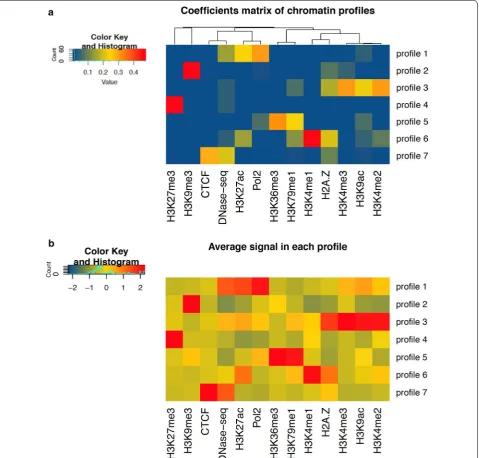
One of the main advantages of the NMF-based approach compared to other chromatin segmentation methods is that the number of combinatorial profiles is not fixed in a predetermined manner, but effectively relies on the extent of correlation among input signals. An intui-tive representation of the seven combinatorial profiles obtained after the NMF procedure is illustrated in Fig. 2.
in H2A.Z, a histone variant involved in the control of the promoter activity and gene responsiveness to spe-cific physiological conditions. While the H2A.Z mark seems to be less represented, histone modifications H3K4me2 and H3K4me3 show the highest contribution to the profile. We also observe a moderate contribu-tion of H3K9ac, a histone-acetylacontribu-tion mark known to be associated with active promoters. A different cluster of
histone modifications is observed in chromatin profile 6. This epigenetic status is predominantly enriched in H3K4me1, which is known to be associated with distal enhancer regions [37]. However, the profile also exhib-its a much more lower content of four additional epige-netic marks (H2A.Z, H3K4me2, H3K27ac, H3K79me1), which is likely to suggest a modest level of chromatin activation.
Chromatin profile 7 apparently lacks any promoter-associated or transcription-promoter-associated histone modi-fication, but shows moderate enrichment in DNase hypersensitive sites and CTCF binding, with a minor contribution in H2A.Z. CTCF is an insulator binding protein that can interact with promoters, enhancers or other types of DNA regulatory elements, activating or repressing the transcriptional machinery according to the type of the bound DNA sequence [38]. Notably, the absence of any acetylation or methylation mark is quite consistent with the functional role of CTCF, which is prevalently found in intergenic sequences, often distant from the transcription start site. This chromatin profile is mostly represented by a combination of CTCF and DNase HS, an epigenetic mark extensively used to map active cis-regulatory DNA elements by identifying chro-matin accessibility regions in the genome [18, 39, 40].
Profile 5 consists of a combination of four differ-ent chromatin marks. Among them, the most preva-lent, H3K36me3, is a tri-methylated histone mark associated with RNA elongation within the body of transcribed genes. Another transcription-associated mark, H3K79me1, also appears in the same profile with a smaller contribution. Other two marks, Pol2 and H3K9ac, are mostly linked to active promoters or other regulatory regions but are more poorly represented than transcription marks H3K36me3 and H3K79me1. The last two epigenetic profiles, 2 and 4, are dominated by the presence of two different repressive chromatin marks, respectively: the histone tri-methylation H3K9me3 and H3K27me3. Profile 2 combines H3K9me3 with very low occurrence of H2A.Z, whereas H3K4me3 and other TSS/transcription-associated marks are almost absent. Chromatin profile 4 shows a high contribution of the histone modification H3K27me3, a well-characterized mark associated with polycomb-mediated repressed regions and promoter inactivation. Interestingly, we found that the chromatin mark composition of profiles 3, 4, 5 and 6 was very similar to that of some profiles (defined as epigenetic ‘codes’) previously obtained in [15] in the same cell line using a slightly different set of histone modifications.
To evaluate the robustness of each epigenetic track in each combination of marks, we also estimated the mean coverage signal of every mark across the different pro-files. As shown in the heatmap of Fig. 2b, the mean signal distributions resemble well the composition of different chromatin profiles as reported in the coefficient matrix (Fig. 2a). Taken together, these results demonstrate the applicability of the NMF approach in discovering com-binatorial information among multiple epigenetic marks, highlighting functional interactions otherwise not easily decipherable using separate ChIP-seq assays.
Genomic distribution of chromatin profiles
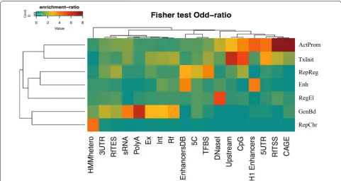
As a first step, we sought to characterize each profile as a function of their genomic their distribution using a set of functional elements and well-annotated regions as benchmark. To define the biological significance of the different profiles, we compared their genomic distribu-tion with those of a number of known funcdistribu-tional regions, including Refseq genes, Refseq promoters, enhanc-ers, poly-adenylation sites, 5′ and 3′ UTRs, smallRNAs, CAGE clusters, transcription factors binding sites and other types of functional genomic data (see “Methods” section). Interestingly, the overlap analysis identified very different patterns of enrichment among the profiles, indicating the presence of distinct epigenetic functions (Fig. 3; Additional file 1: Figure S2).
To provide a more intuitive and biologically interpret-able definition of each profile, we replaced numbers from 1 to 7 with a list of seven distinct ‘genomic labels’ (and abbreviations) on the basis of the different enrichment patterns using the following scheme: chromatin pro-file 1 = ‘Active Promoter’ (ActProm); chromatin profile 2 = ‘Repressed Chromatin’ (RepChr); chromatin profile 3 = ‘Transcription Initiation’ (TxInit); chromatin profile 4 = ‘Repressed Regulatory Regions’; chromatin profile 5 = ‘Gene Body Transcription’ (GenBd); chromatin pro-file 6 = ‘Enhancer Regions’ (Enh); and chromatin profile 7 = ‘Regulatory Elements’ (RegEl).
factors binding sites (f.e. = 1.62, p value = 10−8) and Ref-seq intragenic regions (genes f.e. = 1.9, exons f.e. = 1.55, introns f.e. = 1.62), suggesting a more spread distribution around the gene TSS. Globally, these results demonstrate that both the chromatin profiles are strongly associated with the regions surrounding gene promoters but show inverse patterns of enrichment around the transcription start site, indicating a possible different organization of the chromatin near the 5′ portion of the gene. Com-pared to them, the ‘Gene Body Transcription’ profile shows a completely different enrichment pattern, with a significant overlap over the body and the 3′ end of the gene (Refseq genes f.e. = 3.35, exons f.e. = 2.7, introns f.e. = 2.66, TES f.e. = 1.7, 3′UTR f.e. = 2, poly-A sites f.e. = 6.5). This profile also shows significant association with annotated small RNAs, for which it shows consistent
enrichment (f.e. = 4.02, p value = 10−8), but results strongly depleted in the promoter-associated regions. Chromatin profiles RepChr, RepReg, Ehn and RegEl have very poor overlap with all promoter-related regions, but show the tendency to spread over the intergenic portions of the genome. Despite the prevalence of a repressive mark, profiles RepChr and RepReg show distinct patterns of enrichment when we look at their genomic context. While the former is mostly concentrated toward puta-tive heterochromatin regions (f.e. = 4.2, p value = 10−8), the latter shows preferential enrichment for enhancers (f.e. = 4, p value = 10−8), conserved TF binding sites (f.e. = 3.88, p value = 10−8) and distal chromatin interac-tions (f.e. = 2.28, p value = 10−10), but it results weakly represented in TFBS, CpG islands and Refseq 3′-end regions, thus suggesting a degree of association with
ActProm
TxInit RepReg Enh
RegEl
GenBd RepChr
Fig. 3 Enrichment of chromatin profiles with respect to genomic features. The heatmap represents the enrichment of each chromatin profile (rows) compared to different regions of the gene and distinct types of genomic features in the genome (columns). The enrichment is defined as a log-odd ratio as described in “Methods”. Positive associations (odd-ratio >1) are colored from green/yellow to brown whereas negative associations (odd-ratio <1) are indicated in blue. As shown in the heatmap, each combinatorial profile reveals a distinct pattern of enrichment, thus demonstrating the usefulness of the NMF-approach in the biological interpretation of the different chromatin functions. In this heatmap, each profile is associated to a specific biological label in order to facilitate the mnemonic association between the profile and its functional role on the basis of the observed enrichment (top-bottom): ActProm= Active Promoter (profile 1), TxInit= Transcription Initiation (profile 3), RepReg= Repressed Regulatory Regions (profile 4), Ehn= Enhancer Regions (profile 6), RegEl= Regulatory Elements (profile 7), GenBd= Gene Body Transcription (profile 5), RepChr=
Repressed Chromatin (profile 2). Genomic features indicated in the columns are: CAGE = hESC-H1 CAGE clusters from ENCODE; RfTSS = Refseq Transcription Start Sites; RfTES = Refseq Transcription End Sites; 5UTR=Refseq 5’untranslated region; 3UTR = Refseq 3’unstranslated regions; H1 Enhancers = Superenhancer regions from hESC; CpG = CpG islands; Upstream = 1Kb upstream regions from Refseq TSSs; DNase1 = hESC DNase1 Hypersensitive sites from ENCODE; TFBS = Conserved transcription factor binding sites from the Transfac Matrix Database; 5C = Chromatin confor-mation capture carbon copy data from hESC; EnhancersDB = experimentally validated enhancer elements from the VistaEnhancer Dabatabse; Rf
inactive or poised enhancers. Profile RegEl (the CTCF/ DNase HS profile) is strongly associated with open chro-matin accessibility regions (f.e. = 5.2, p value = 10−10), suggesting an association with different types of cis-reg-ulatory DNA elements (insulators, silencers, etc.) and a role in the organization of the chromatin structure. The last combinatorial profile Ehn significantly correlated with both the enhancer groups (Vista Database Enhanc-ers f.e. = 3.83, p value = 10−8, hESC super-enhancers f.e. = 3.9, p value = 10−10), where it shows higher lev-els of overlap compared to profile RepReg. Interestingly, we found that profile ActProm is also significantly asso-ciated with hESC active enhancers, with even higher enrichment than the ‘Enhancer’ profile (f.e = 4.6, Fisher p value = 10−10). It is noteworthy that, in contrast with Enh, the ActProm profile seems to be confined to active enhancers only, as suggested by the extremely poor over-lap with the Vista Database annotation. This different enhancer pattern is likely to suggest that, within enhancer regions, the two profiles are often correlated and, while the presence of Ehn profile is crucial for enhancer predic-tion, the addition of ActProm could help in discriminat-ing between the active and the poised enhancer state.
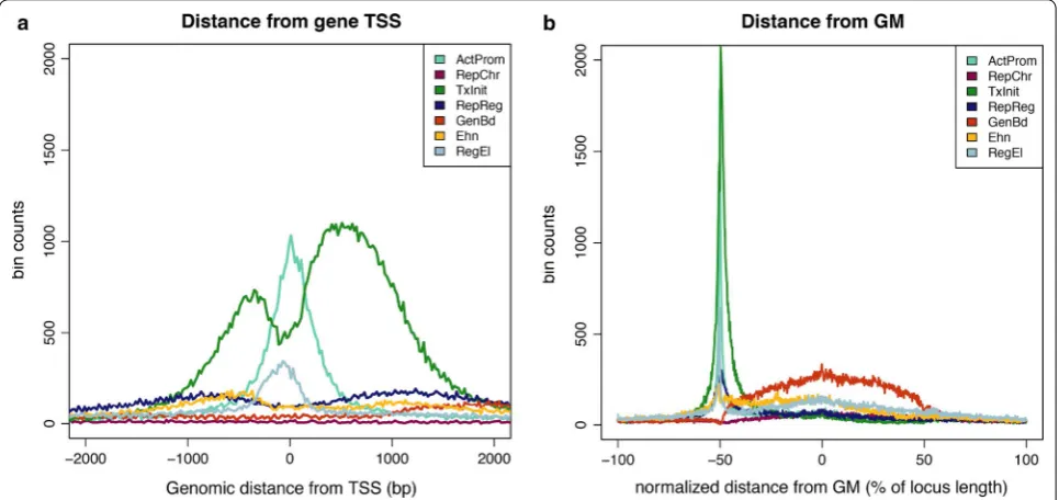
To get a more detailed view of chromatin profiles occurrences in the gene structure, we also investigated how chromatin profiles are differentially distributed around specific structural elements, such as the TSS and
the middle point of the gene. Hence, each combinato-rial profile was analyzed with respect to its distance from the closest gene feature (Fig. 4a, b). Around the TSS, the most striking difference is observed between the two promoter-associated profiles, ActProm and TxInit. These chromatin profiles occur with highest frequency compared to all other profiles, but show completely dis-tinct shapes over a region of 4 Kb surrounding the 5′end of the gene (Fig. 4a). While ActProm precisely maps to the transcription start site, chromatin profile TxInit tends to be broadly distributed both in the upstream and downstream directions, with two large peaks in the TSS surrounding region and a characteristic dip exactly over-lapping the TSS (Fig. 4a).
To investigate spatial relationships among the dif-ferent profiles, we also examined the frequency with which a given profile consecutively occurs next to each other considering all possible pairwise combinations. For any transition A–B, we estimated its occurrence as the logarithmic fold-change of the frequency observed in the real data over the frequency in the random data-set (Additional file 1: Figure S3). Notably, the analy-sis reveals the presence of a low number of meaningful associations. Among these, transition from chroma-tin profile TxInit to ActProm shows the highest level of enrichment (logFC = +1.07). The reciprocal transition ActProm-> TxInit is weakly enriched (logFC = +0.45)
relative to the random profile distribution. Among the most recurrent profile combinations, transition from TxInit to Ehn seems to be also slightly favored (logFC = +0.80). Transition RegEl-> Ehn (+0.37) and ActProm-> Ehn (+0.77) also occur with higher frequency than randomly expected, but show lower occurrence rel-ative to the most frequent profile combinations.
Recovery power of chromatin profiles for a known set of genomic features
We next evaluated the ability of the different chromatin profiles in correctly recognizing distinct classes of known functional elements and comparing their performance with that of most representative epigenetic marks. For this task, we focused on a small set of functionally relevant regions of the gene that are already supported by a consist-ent amount of experimconsist-ental information: the Refseq TSS, the 1-Kb upstream region from the gene TSS, enhancer regions and RNA poly-adenylation sites. For each region, the predictive power of chromatin profiles was assessed using a ROC (receiver operating characteristic) curve (Fig. 5a–c; Additional file 1: Figure S4). To test the per-formance in the Refseq TSS prediction, we focused on a list of 11,263 transcription start sites supported by hESC-H1 CAGE cluster data (i.e., Refseq promoter regions over-lapping at least one CAGE cluster in a window of ±50 bp around the transcription initiation site). We found that, in almost all cases, chromatin profiles showed better perfor-mance compared to that of single chromatin marks, con-firming the ability of NMF in identifying combinatorial interactions that are more informative than single mark contributions. Here, chromatin profile ActProm shows a performance similar to that of the CAGE clusters, but outperforms predictions based on TSS-associated marks (H3K4me3, H3K9ac, Pol2) and those of other mark com-binations. Similarly, profile TxInit shows the best perfor-mance in correctly predicting 1-Kb regions upstream of the Refseq TSS (Fig. 5b), with higher recovery power com-pared to the performance of promoter-associated marks. Notably, the analysis of enhancer predictions (Fig. 5c) shows that, at relatively lower false positive rates (<0.25), the ‘Enhancer’ profile and the ‘Repressed Regulatory’ pro-file slightly outperform predictions from H3K4me1 mark and other related histone modifications such as H3K4me2 and H3K27ac. In contrast, no improvement was observed when we compared the performance of profile GenBd with the predictive power of the H3K36me3 mark (Addi-tional file 1: Figure S4).
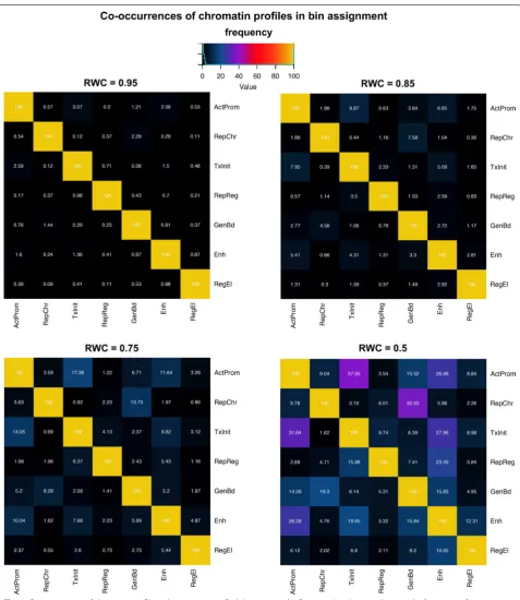
Ambiguousness in chromatin profile assignment
We also set out to assess how confidently a profile could be univocally assigned to each bin by simply taking the dominant (i.e., the maximum) weight observed in the W(j,
c) matrix for that bin. For assessing the robustness this relationship, we defined the relative weight contribution (RWC) of each profile in a given bin. We estimated the RWC by simply normalizing the weights of W for the bin on the profile with the maximum contribution, which cor-responds to Rw(j,c)=W
j,c /max
W
j,
We then asked how the assignment of additional pro-files influences the amount of genomic information cap-tured in each combinatorial pattern. For this purpose, we examined how the mean overlap rate with genomic annotations varies in function of the mean number of profiles assigned per bin (Additional file 1: Figure S5). The mean overlap rate was estimated as the percentage of regions of a given feature covered by a given profile
over the total sequences of that feature, averaged across all genomic features significantly enriched in the profile (Fig. 3; Additional file 1: Figure S2). We found that, for some profiles (‘Repressed Regulatory,’ ‘Regulatory Ele-ments’ and ‘Repressed Chromatin’) the degree of overlap constantly increases until all the profiles are assigned, suggesting that the profiles are distributed with a lower degree of clustering with respect to the genomic elements
considered. Conversely, profiles ActProm, TxInit, GenBd, Ehn show a flection point between three and four, indi-cating that assigning at least two other profiles per bin
can add further information with an increase of overlap that is, on average, between 7% (‘Enhancer’) and 13% (‘Transcription Initiation’).
Association between chromatin profiles and gene expression
We decided not to include transcriptomic data from RNA-seq experiments as input signal for the NMF analysis. The RNA-seq expression estimates from the ENCODE consortium database in hESC-h1 were instead used to test whether the different profile distributions are associated with the transcriptional activity and can be functionally interpreted. Specifically, we examined whether the occurrence of specific chromatin profiles over pre-defined gene boundaries correlates with the corresponding expression levels (RPKM). To this aim, we computed the frequency of each chromatin profile over a region of 12 kb (2-kilobases upstream and 10-kilo-bases downstream) spanning the transcription start site, binned them in increasing ranges of expression levels and identified the most frequent profile in a given bin for a given expression interval. We observed that most of the epigenetic profiles are partitioned in a number of well-delimited regions along the genomic and the expression coordinate, generating diverse bi-dimensional patterns that reflect multiple levels of information about the gene position and the promoter activity (Additional file 1: Figure S6). On a global scale, these bi-dimensional pat-terns clearly indicate that chromatin profiles can be not only associated with distinct gene elements but are also informative about the transcriptional status of the gene. The frequency distribution for separate chromatin pro-files is reported in Additional file 1: Figure S7.
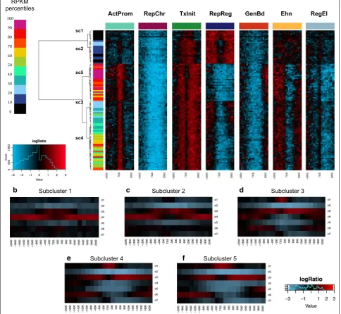
Chromatin profiles are organized in enrichment patterns that reflect distinct levels of transcription
Encouraged by these observations, we asked if the fre-quency distribution of single profiles could be used to identify enrichment patterns able to discriminate the dif-ferent ranges of expression. We assigned each gene to a different expression percentile interval on the basis of the corresponding RPKM (reads per kilobase per million of mapped reads). Next, we computed the frequency of each chromatin profile in each expression interval in each bin over a window of ±2 kb around the transcription start site. We next estimated the logarithmic fold-change of the occurrence observed in the real data with respect to the frequency in the random dataset. The heatmap in Fig. 7a clearly shows that, along the genomic and the expression coordinate, chromatin profiles follow differ-ent enrichmdiffer-ent shapes that resemble well their genomic distribution, consistently with our previous findings (see Fig. 3, 4; Additional file 1: Figure S6). Moreover, hierar-chical clustering analysis of the percentile intervals iden-tified a number of clusters and subclusters that accurately reconstruct the full scale of expression. In particular, the clustering analysis allowed us to identify five expression
subclusters (Fig. 7a; Additional file 1: Figure S8) spe-cifically associated with a diverse pattern of enrichment (Fig. 7a), thus suggesting a correlation between the occurrence of each profile and the extent of transcrip-tional activity. Furthermore, expression subclusters are differentially marked by precise sequences of (enriched) profiles around the gene TSS. In particular, five pat-terns (Fig. 7b–f), discriminate well between the different expression level groups.
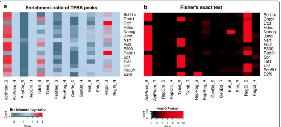
Association between chromatin profiles and transcription factor binding data
for several TFs (Fig. 8b) (Bcl11a: f.e. = 1.6, p value = 10−5; Hdac: f.e. = 2.14, p value = 10−6; Nanog: f.e. = 1.81, p value = 10−5; Nsrf: f.e. = 2.4, p value = 10−5; p300:
f.e. = 1.12, p value = 10−4; Usf: f.e. = 2, p value = 10−5; Pou5f1: f.e. = 1.45, p value = 10−15) but with lower lev-els of overlap than found in promoter-associated profiles
a
f
b Subcluster 1 c Subcluster 2 d
e Subcluster 4 Subcluster 5
Subcluster 3 Fold-enrichment of chromatin profiles within +/- 2kb around the TSS
ActProm RepChr TxInit RepReg GenBd Ehn RegEl
sc1
sc2
sc5
sc3
sc4 RPKM
percentiles 100
90 80 70 60 50 40 30 20 10 0
(ActProm and TxInit). In contrast, the RegEl profile is found to be enriched in the CCCTC binding insulator protein (CTCF: f.e. = 116, p value = 10−12) and the dou-ble-strand break repair Rad21 homolog protein (Rad21: f.e. = 121, p value = 10−12), another chromatin binding protein known to cooperate with the CTCF-mediated insulator complex in modulating enhancer–promoter interactions [43].
Comparison with different chromatin segmentation approaches
We compared our chromatin profile distribution with that of ChromHMM (9), which is a common chroma-tin segmentation technique. We did not compare our method with the Segway algorithm [10] because its 1-bp segmentation resolution would not permit to easily com-pare the different profile/state distributions.
Both ChromHMM and EpicSeg have been shown to be effective when used close to 13 chromatin states [11, 44]. Therefore, an additional NMF model with a factorization rank of 13 was also tested for the comparison. This is also the maximum number of states we can compute since it corresponds to the number of epigenetic marks in the input data matrix.
We assessed the ability of the methods to recover func-tional information about biologically relevant regions and to correctly predict the presence of distinct functional
elements in terms of their sensitivity (true positive rate), specificity (true negative rate), precision (number of true positives divided by the sum of true positives and false positives) and accuracy (total fraction of correct predictions).
The heatmaps in Additional file 1: Figure S9 show the enrichment of the epigenetic profiles (states) gen-erated by NMF with r = 7 (denoted as NMF7), NMF with r = 13 (NMF13), the ChromHMM 7-states model
(ChromHMM7) and the ChromHMM 13-states
model (ChromHMM13). The enrichment patterns of NMF7 are very similar to those of ChromHMM7 and ChromHMM13, while the NMF13 model is much less effective, confirming that a level of factorization of 7 is sufficient for the NMF model to capture the combinato-rial information contained in the chromatin profiles.
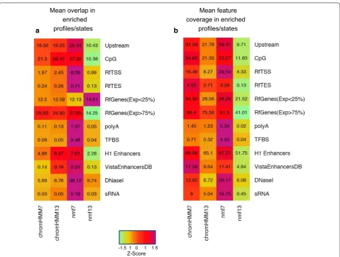
Figure 9 illustrates the ability of each method to retrieve annotated features. We restricted the analy-sis to all the combinatorial profiles (states) that were significantly enriched in a given feature, and used the enriched profiles (states) to determine the degree of genomic overlap. Specifically, the amount of infor-mation retrieved was measured using two different indicators: (i) the mean profile/state overlap and (ii) the mean feature coverage. The mean profile over-lap was computed as the fraction of bins of a profile P overlapping at least one element of the feature G,
Fig. 8 Overlap between chromatin profiles and putative TF binding sites from hESCH1 ChIP-seq data. a The heatmap shows the extent of overlap between ChIP-seq peaks from each transcription factor (along rows) and the distribution of a given chromatin profile in both the observed and the random data (columns). For each possible combination of TF/profile, a fold-enrichment is calculated following the procedure described in “ Meth-ods”. b Heatmap showing the significance of the enrichment for the same combinations of TFs/profiles represented in (a). The color-scale indicates the associated p value on the basis of the Fisher’s exact test (reported in the −log10 form): black: p > 0.01; brown 0.01 > p > 0.0001; dark red 0.0001 >
averaged across all profiles/states enriched in that feature. The mean feature coverage was estimated as the fraction of elements in G matching the profile P, averaged across all profiles/states found to be signifi-cantly enriched in that feature. We observed that the two indicators gave similar results when we looked at the performance between the different techniques (Fig. 9a, b). Compared to our NMF model and Chrom-HMM approaches, the NMF13 model shows very weak overlap in all the features examined (Fig. 9a), with the exception of low expressed Refseq genes (mean profile
overlap = 14.6%). A significant drop of overlap from NMF7 to NMF13 is also observed in terms of mean fea-ture coverage (Fig. 9b), which is in accordance with our previous results.
Interestingly, we noted that our NMF7 model slightly outperforms ChromHMM7 and ChromHMM13 both in terms of profile/state overlap and feature coverage for almost all the features considered (Fig. 9a, b). Indeed, the NMF7 model exhibits the highest overlap rate in 11 out of 12 features (91%). Remarkably, the NMF7 approach and the ChromHMM7 tend to perform better than the
b a
-1.5 1 0 1 1.5 Z-Score Mean overlap in
enriched profiles/states
Mean feature coverage in enriched
profiles/states
Fig. 9 Overlap and coverage levels of different genomic elements using enriched profiles/states in each method. Chromatin segmentation approaches are reported in columns, genomic features in rows. Each cell in the heatmap indicates the amount of overlap (a) or coverage (b) observed intersecting a feature with any profile/state specifically enriched in that feature using NMF or ChromHMM-based methods. The extent of overlap is represented as the mean percentage by which an enriched profile/state overlaps the feature (a). Similarly, we represent the cover-age as the mean percentcover-age of a given feature covered by any enriched profile/state. The color-scale (from green to purple) mirrors the amount of information retrieved for each pair of feature/method. Genomic features labels indicate: Upstream = 1kb upstream region from the Refseq TSS; CpG
ChromHMM13 model in terms of feature coverage. In 9 out of 12 features (75%), our NMF model shows the best mean coverage, confirming the ability of the NMF profiles to retrieve a larger fraction of biological information from distinct types of functional regions in the genome. In both analyses, the most striking differences are observed for Refseq transcription start sites (mean overlap: NMF7 : 8%, ChromHMM7 : 1.97%, ChromHMM13 : 2.45%; mean coverage: NMF7 : 23.5%, ChromHMM7 : 16.4%, ChromHMM13 : 8.2%), upstream regions (mean overlap: NMF7 : 26.3%, ChromHMM7 : 18.5%, ChromHMM13 : 19.2%; mean coverage: NMF7 : 39.3%, ChromHMM7 : 31.9%, ChromHMM13 : 21.8%), smallRNAs (mean over-lap: NMF7 : 0.18%, ChromHMM7 : 0.03%, ChromHMM13 : 0.05%; mean coverage: NMF7 :16.7%, ChromHMM7 : 8%, ChromHMM13 : 5%) and DNase hypersensitive sites (mean overlap: NMF7 : 38.1%, ChromHMM7 : 5.6%, ChromHMM13 : 8.7%; mean coverage: NMF7 : 20.1%, ChromHMM7 : 12.6%, ChromHMM13 = 6.7%).
To assess the generality of these observations, we repeated the two analyses illustrated above varying the set of enriched profiles/states used for each method. We considered all possible combinations of size L ≤ N among the profiles/states, where N corresponds to the total number of enriched profiles/states detected by a given method in a given feature (Additional file 1: Table S1). The distribution of the mean profile overlap and the mean feature coverage generated for each feature are shown in Additional file 1: Figure S10. We found that, in almost all cases, the NMF7 approach gives similar or better overlap compared to both the ChromHMM7 and the ChromHMM13 model, suggesting that this trend is unlikely to depend on the selection of a specific combina-tion of enriched profiles (Addicombina-tional file 1: Figure S10a, b).
Next, we tested the performance of the different approach in the prediction of some important functional genomic features (TSSs, upstream regions, and puta-tive H1 enhancers) using, for each model, the full set of enriched profiles/states. The true positive rate was esti-mated considering all the bins assigned to any of the enriched profile/state and having (or not) a minimum overlap (1 bp) with the analyzed feature. A number of intragenic (or intergenic) intervals lacking any annotation for the specific feature were assumed as negative con-trols for the test. We found that, when all the enriched profiles/states were used, our approach has in general the same predictive power of the ChromHMM models (Additional file 1: Figure S11a–c). We also observed that, in the prediction of the Refseq TSSs (Additional file 1: Figure S11a), the NMF7 model shows a marginal drop in sensitivity and a small gain in precision and specific-ity compared to ChromHMM-based approaches. As an
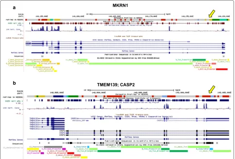
example, a UCSC Genome Browser representation of the chromatin profile distribution generated by the NMF7 model at level of two distinct genomic regions on the human chromosome 7 (the TMEM139/CASP2 genomic loci and the MKRN1 locus) is reported in Fig. 10.
Chromatin profiles distribution in IMR90 ENCODE data
We also tested the NMF approach on a different human dataset, i.e., IMR90 (fetal lung fibroblasts), another cell line well characterized by a large number of functional chromatin assays publicly available on the ENCODE catalog [5]. We compared the results on the two datasets using both an IMR90-derived coefficient matrix (H) and that derived from the hESCs-H1 cell line. A Pearson cor-relation analyses was performed using all possible pair-wise comparison between the profiles (Additional file 1: Figure S12a, b). We found that, in both cases, most of the IMR90 profiles are well correlated with the corre-sponding hESC profile (as suggested by the red diagonal in the Additional file 1: Figure S12a, b), indicating that the two datasets tend to be similar in terms of genomic organization and chromatin mark composition. The only major difference is observed for the profile RepReg. In hESCs, this epigenetic profile is mainly dominated by the H3K27me3 histone modification with almost no traces of other mark contributions (Fig. 2a). Conversely, the IMR90 profile s4 is described by moderate H3K79me1 and CTCF mark contributions (data not shown) and par-tially correlates with the hESC profiles GenBd and RegEl. In contrast, we found that hESC RepReg profile appears closer to the IMR90 profile ‘s2,’ which is represented, indeed, by a combination of the two repressive marks H3K27me3 and H3K9me3.
Discussion
In this work, we demonstrated the usefulness of the non-negative matrix factorization for the systematic characterization of the chromatin functions. This is an unsupervised classification technique that uses a signal decomposition algorithm to reduce the dimensionality of multivariate datasets to a restricted number of com-binatorial components [14, 45, 46]. The ability of NMF to use the sparse data makes the approach particularly appropriate for the analysis of NGS experimental data. We show here that the method can discover functional relationships among different epigenetic marks and per-mits to extract a number of combinatorial profiles useful for the biological interpretation of the broad spectrum of the chromatin functions.
combinations of marks. One of the main advantages of the NMF approach is that the number of chromatin pro-files is not arbitrarily set. Indeed, here we statistically assessed the stability of the data for an increasing num-ber of profiles and selected the value at which the clus-tered data started being significantly stable compared to the random profile distribution. This approach allowed us to identify seven different chromatin profiles that bet-ter represents the most recurrent combination of marks. We tested NMF on a combined epigenetic dataset of 13 chromatin marks, encompassing 9 histone modifications,
one histone variant, two transcription factors binding data (Pol2, CTCF) and one chromatin accessibility mark (DNase hypersensitive site assay), previously mapped in hESC and IMR90 lines. A complete list of the analyzed datasets is reported in the Additional file 2. We found that epigenetic profiles are composed by different chro-matin patterns that resemble quite well the functional diversity of single marks, highlighting the ability of NMF in capturing spatial relationships among different epi-genetic signals. When compared to a number of well-annotated features and other functional elements, we
a
b
MKRN1
TMEM139; CASP2
also found that combinatorial profiles are predominantly associated with specific genomic contexts, which sug-gests the usefulness of the NMF approach in extracting biologically interpretable information from meaningful combinations of marks.
We also found that chromatin profiles are more effec-tive than single marks in recovering known functional elements and observed that most profiles are distrib-uted following specific bi-dimensional patterns along the genomic and the expression coordinates. This strongly suggests that chromatin profiles are not only related to the genomic localization of distinct functional elements but can also be correlated to the level of transcriptional activity. Specifically, we showed that, around the pro-moter region, chromatin profiles are organized in signa-tures that preserve positional information and are able to mirror well the different ranges of expression. Our data suggest the presence of an almost symmetric mecha-nism of chromatin activation, which could propagates progressively from the gene TSS toward distal upstream and downstream regions through a defined number func-tional chromatin states (Fig. 7b–f). When compared to those obtained from ChromHMM, our combinatorial profiles share similar patterns of enrichment in terms of genomic organization, but tend to have better sequence overlap with a variety of functional elements.
We also used the enriched profiles from both methods to verify how well they can predict annotated regions in the genome and showed that the NMF model has very similar predictive power, but has a slightly higher preci-sion and specificity in the prediction of Refseq TSSs, with a very small drop in terms of sensitivity.
Furthermore, our results are not specific for the selected cell line (hESC-H1) since the profiles obtained using another one (IMR90) provides very similar results.
Despite these observations, there are still a number of limiting factors that have to be taken into account and that will require additional efforts to further improve the accuracy of the approach. First of all, we analyzed how the chromatin profile assignment varies as function of the single profile contribution and we found that spe-cific profile combinations are more recurrent than oth-ers, suggesting that there is still a fraction of uncertainty in determining the correct chromatin status for specific groups of bins. We also found that, in some cases, assign-ing more than one profile makes the chromatin segmen-tation procedure even more informative, suggesting that some genomic information could be missed in the bin assignment. In this context, more statistically rigorous approaches to redefine bin/profile relationships will likely be needed. Moreover, further methodological improve-ments will be required to optimize the signal decompo-sition algorithm in the integrative analysis of multiple
epigenetic datasets. Although the technique has been shown to be effective in capturing most important func-tional mark interactions, the detection of combinatorial information for some histone mark distributions (as for H3K27me3, H3K9me3 and H3K4me1) still remains a challenging task. This consideration arises from the fact that such histone modifications tend to be compressed into a unique chromatin profile (as for RepReg, RepChr, Ehn) rather than gradually fluctuate over different func-tional states, making the approach less sensitive to local patterns of mark interactions. An example of such pat-terns is particularly evident in undifferentiated cells, where distinct bivalent domains of chromatin modi-fications (e.g., H3K27me3/H3K4me3 and H3K4me3/ H3K9me3) were found at poised promoters of lineage-specific genes [47, 48]. This limitation, however, seems not to be strictly related to the NMF approach as a simi-lar trend also arises with previously proposed chromatin segmentation techniques [9–11, 49], thus indicating that a certain degree of complexity still persists in the inter-pretation of this kind of data
Another common limiting factor is represented by the large amount of memory and time resources required to process such large amount of epigenetic signals, which often makes the analysis not very practical. For the hESC dataset, both the NMF and the ChromHMM performed in the same time range on a Intel®Xeon® 56 Gb RAM multi-core machine. It is, however, worth mention-ing that the implementation of the NMF technique in the R environment allows easier integration of statisti-cal function and appropriate libraries normally used in downstream analyses. We believe that this technique can improve the limited repertoire of tools and algorithms currently available in the analysis of high-dimensional epigenetic datasets, thus facilitating the development of novel frameworks for a more accurate characterization of the chromatin activity (the implemented pipeline is pro-vided in Additional file 3).
Conclusion