Introduction to MATLAB
Brett Ninness
Department of Electrical and Computer Engineering
The University of Newcastle, Australia.
The name ‘MATLAB’ is a sort of acronym for ‘Matrix Laboratory’. In fact, MATLAB is an interpreted language which is designed for calculations with matrix and vector quantities.
Software of this sort turns out to be very useful in the area of signal and systems analysis. This is because a signal can be represented as a vector of values that the signal takes as it evolves over time, and also because the effect of systems on this signal can be represented by the operation of matrix multiplication on the vector signal representation.
The fact that MATLAB is an interpreted language means that commands to it are parsed and executed as they are entered; there is no need for the compilation/link/run phases that are necessary in, for example, ‘C’ or fortran programming. At the same time, with MATLAB it is also possible to have something like a ‘C’ or fortran programme, complete with conditional loops, subroutines and GUI interfaces. This is achieved via what are known as MATLAB ‘script’ and ‘function’ files.
This section will provide an introduction to MATLAB for readers who have never encountered it before. It is intended to be read in front of a computer running MATLAB so that ideas can be tried by the reader as they are explained in the text.
1
Starting MATLAB
How MATLAB is invoked depends on which operating system you are running, and is really an issue for you to discuss with you system manager or tutor. However, if it is installed on a Microsoft branded operating system you have access to, then invoking it will involve double clicking an icon on your desktop, or accessing it from the ‘applications’ menu. If it is installed on a unix operating system you have an account on, then typing ‘matlab’ at the command prompt should invoke it.
2
MATLAB Interaction
Once MATLAB is invoked, it will present you with a ‘command window’ in which instructions may be entered. This window will initially look something like this:
< M A T L A B >
Copyright 1984-1999 The MathWorks, Inc. Version 5.3.1.29215a (R11.1)
Oct 6 1999
To get started, type one of these: helpwin, helpdesk, or demo. For product information, type tour or visit www.mathworks.com.
>>
1. The prompt that the MATLAB command interpreter is ready for a command is
>>
Anything typed on the keyboard at this point will be echoed after this prompt and then interpreted and executed when the ‘enter’ key is hit.
2. If help is needed, then this can be obtained by entering commands such ashelpwinorhelpdesk; actually justhelpwill do.
To quit from MATLAB, typequitat the command prompt:
>> quit
3
Entering Vectors and Matrices
As already mentioned, the fundamental data types that MATLAB is designed to handle are vectors and matrices of floating point values (although other data types such as character strings, structures, and objects with overloaded operations are also possible). For example, the vector
x=
1 2
can be entered into the MATLAB workspace via the command
>> x=[1;2]
x =
1 2
There are three points to note here
1. The square brackets[and]are used when entering vector/matrix values;
2. The semi-colon symbol;is used to denote the end of a row of a vector (or matrix);
3. The elements entered into the vector are echoed back to the screen once entered.
The echoing operation can be inhibited by using the semicolon;at the end of a command:
>> x=[1;2]; >> x
x =
1 2
Notice that it was only whenxwas entered without a terminating;that it was echoed.
While;is used to denote the end of a row, the comma,(or simply just a space) denotes the end of a column, so that a row vector can be entered as so
>> y = [3,4]
y =
Having a means for terminating both rows and columns means that matrices can be entered. For example,
A=
1 2 0 3
is entered as
>> A = [1,2;0,3]
A =
1 2
0 3
An important point is that matrix/vector blocks can be concatenated together using the column delimiter,
and the row delimiter;. For example, a matrix can be stacked on top of a row vector
>> [A;y]
ans =
1 2
0 3
3 4
and a column vector can be placed before a matrix
>> [x,A]
ans =
1 1 2
2 0 3
Finally, once a matrix or vector is specified, its row and column dimension can be found using thesize
operator
>> size([x,A])
ans =
2 3
From this example, thesizeoperator clearly returns two numbers (as a row vector), the first being the number of rows, and the second being the number of columns. What if you forget what order thesize
operator returns row and column information? This question provides an ideal opportunity to illustrate a general principle with MATLAB - if you want help, ask for it with thehelpcommand:
>> help size
SIZE Size of matrix.
D = SIZE(X), for M-by-N matrix X, returns the two-element
row vector D = [M, N] containing the number of rows and columns in the matrix. For N-D arrays, SIZE(X) returns a 1-by-N
vector of dimension lengths. Trailing singleton dimensions are ignored.
separate output variables. [M1,M2,M3,...,MN] = SIZE(X) returns the length of the first N dimensions of X.
M = SIZE(X,DIM) returns the length of the dimension specified by the scalar DIM. For example, SIZE(X,1) returns the number of rows.
See also LENGTH, NDIMS.
Overloaded methods help zpk/size.m help tf/size.m help ss/size.m help frd/size.m
4
Entering Structured Vectors and Matrices
MATLAB has several commands and syntax options that allow for streamlined generation of various com-mon vector and matrix structures. For example, vectors and matrices of all ones or zeros are entered by specifying the dimensions of the vectors or matrices required
>> z = zeros(1,4)
z =
0 0 0 0
>> B = ones(2,3)
B =
1 1 1
1 1 1
An important matrix is the identity matrixI which is specified by theeye command together with an indication of the dimension required (note, in this case, since an identity matrix must be square and hence have equal row and column dimension, then the function generating an identity matrix needs only one argument)
>> I = eye(2)
I =
1 0
0 1
More general diagonal matrices are specified using thediagoperator in conjunction with a specification of the diagonal values
>> C = diag([3,4])
C =
3 0
Thediagoperator also performs the reverse operation of extracting the diagonal entries of a matrix
>> diag(C)
ans =
3 4
Finally, a vector composed of a start valuea, an end valueband all points in-between that are spacedt
units apart is specified using the colon:operator asa:t:b. For example
>> c = 1:0.2:2
c =
1.0000 1.2000 1.4000 1.6000 1.8000 2.0000
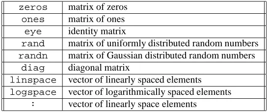
A list of the matrix/vector building tools available in MATLAB is given in table 1, where several cases that were not discussed here (but will be explained later in this book).
zeros matrix of zeros
ones matrix of ones
eye identity matrix
rand matrix of uniformly distributed random numbers
randn matrix of Gaussian distributed random numbers
diag diagonal matrix
linspace vector of linearly spaced elements
logspace vector of logarithmically spaced elements
: vector of linearly space elements
Table 1: MATLAB Matrix/Vector Building tools.
5
Matrix/Vector Operations
The essential feature of MATLAB is that operations on these matrix and vector elements are now very streamlined. For example, provided the matrix/vector dimensions are compatible, then matrix/vector mul-tiplication is easy and returns a quantity of the appropriate dimension
>> x*y
ans =
3 4
6 8
>> y*x
ans =
11
ans =
5 6
>> y*A
ans =
3 18
Note that if a mistake is made and a multiplication is attempted with quantities of incompatible dimension, then an error message is generated
>> A*y
??? Error using ==> *
Inner matrix dimensions must agree.
There are several other basic Matrix/Vector operations available.
For example, addition and subtraction uses the+and-symbols as expected
>> A*x-x
ans =
4 4
>> A*x+x
ans =
6 8
A matrix can be raised to a power by using theb operator,
>> Aˆ3
ans =
1 26
0 27
which can be checked as follows
>> A*A*A
ans =
1 26
0 27
>> y
y =
3 4
>> y’
ans =
3 4
>> A
A =
1 2
0 3
>> A’
ans =
1 0
2 3
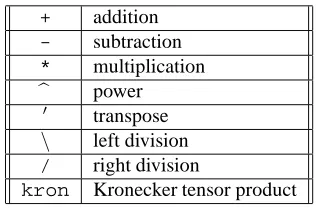
In summary then, MATLAB provides the following basic matrix/vector operations as shown in table 2. The division and tensor product operators are somewhat advanced and hence are not addressed here.
+ addition
- subtraction
* multiplication
b power
0 transpose \ left division
/ right division
kron Kronecker tensor product
Table 2: MATLAB Matrix/Vector Operations
6
Element-wise operations
As is hoped the reader already knows, algebraic operations on matrices and vectors can be quite different to those on scalars. Some operations, like matrix addition and subtraction are very straightforward, since they are defined elementwise. That is, for matricesAandC,A+CandA−Care new matrices whose elements are just the sum and difference of the corresponding elements inAandC. That is, ifD=A+C, thenD(1,1) =A(1,1) +C(1,1)
ans =
4
>> A(1,1)+C(1,1)
ans =
4
This same sort of simplicity does not hold for other matrix operations. In particular, with matrix multipli-cation, ifD=A∗C, then (for example)D(1,2)6=A(1,2)∗C(1,2)
>> D=A*C; D(1,2)
ans =
8
>> A(1,2)*C(1,2)
ans =
0
However, it is often useful to be able to force an operation to be elementwise, and MATLAB achieves this by preceding an operation this is to be forced by the period.like so
>> D=A.*C; D(1,2)
ans =
0
This means that matrix multiplication, which under the normal matrix/vector definition is only possible when the column dimension of the left multiplicand equals the row dimension of the right multiplicand, now applies (if elementwise operation is specified) when the row and column dimensions of the two mul-tiplicands are equal
>> [1;2]*[3;4]
??? Error using ==> *
Inner matrix dimensions must agree.
>> [1;2].*[3;4]
ans =
3 8
The matrix power operatorb can also be made to operate elementwise by preceding it with a period
>> [1,2,3].ˆ2
ans =
7
Selecting Matrix/Vector Elements
Once the elements in a matrix or vector are entered, it is possible to then select these elements via specifying their co-ordinates in the matrix or vector.
For example, with a vector, the element number is specified
>> x
x =
1 2
>> x(1)
ans =
1
>> x(2)
ans =
2
while for a matrix, two co-ordinates are required - the row and column number:
>> A
A =
1 2
0 3
>> A(1,1)
ans =
1
>> A(1,2)
ans =
2
More than one element can be selected if the row and/or column indices are themselves vectors of multiple entries. For example, with vectors only one range of co-ordinates needs to be specified:
>> c
c =
1.0000 1.2000 1.4000 1.6000 1.8000 2.0000
ans =
1.2000 1.4000 1.6000
while with matrices, both row and column ranges are needed
>> A
A =
1 2
0 3
>> A([1;2],1)
ans =
1 0
>> A([1;2],2)
ans =
2 3
Actually, there is a very useful shorthand notation in MATLAB for the whole column of a matrix - the colon:represents a column, so that the above examples can be shortened to
>> A(:,1)
ans =
1 0
>> A(:,2)
ans =
2 3
This:operation allows for an interesting and extremely useful MATLAB trick that forces a vector to be a row vector by selecting its elements and then putting them in a column
>> y
y =
3 4
ans =
3 4
8
Pre-defined constants
When MATLAB starts, certain variable names are initialised with values that are commonly required. For example the variable namepiis initialised to the valueπ
>> pi
ans =
3.1416
whileiandjare both initialised toi=j=√−1 >> j
ans =
0 + 1.0000i
Finally,epsis initialised to a value that varies from computer to computer. It is (essentially) a measurement of the finest granularity of floating point representation that the computer you are using is capable of
>> eps
ans =
2.2204e-16
For any of these pre-defined variables, it is possible to overwrite them
>> i
ans =
0 + 1.0000i
>> i=5; >> i
i =
5
However, as a general rule, it is best to avoid this. In particular, it can be very dangerous to overwriteeps, since some MATLAB library programmes depend on this variable being set to its initialised value.
9
Fundamental Scientific Functions
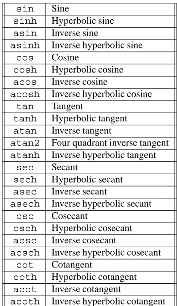
MATLAB has a number of built in scientific functions such as you would expect to find on a scientific calculator. A complete list is given in tables 3 and 4 which break the scientific function list into those of trigonometric and exponential sort.
>> sin(pi/4)
ans =
0.7071
orelogπ
>> exp(log(pi))
ans =
3.1416
is, as just illustrated, simply a matter of entering the required calculation. However, the important point is that these functions work element-wise on vectors and matrices as well. For example
>> theta=0:pi/4:pi
theta =
0 0.7854 1.5708 2.3562 3.1416
>> sin(theta)
ans =
0 0.7071 1.0000 0.7071 0.0000
10
Complex Numbers and Functions
One of the particularly useful feature of MATLAB is that it transparently handles operations with complex valued quantities. Any element of a matrix can be complex, and operations on that matrix will then take account of the elements being complex. For example
>> F = [1+j,1-j;2,exp(j*pi)]
F =
1.0000 + 1.0000i 1.0000 - 1.0000i
2.0000 -1.0000 + 0.0000i
>> log(F)
ans =
0.3466 + 0.7854i 0.3466 - 0.7854i
0.6931 0 + 3.1416i
As another example, we could check De-Moivre’s Theorem
ejθ= cosθ+jsinθ
sin Sine
sinh Hyperbolic sine
asin Inverse sine
asinh Inverse hyperbolic sine
cos Cosine
cosh Hyperbolic cosine
acos Inverse cosine
acosh Inverse hyperbolic cosine
tan Tangent
tanh Hyperbolic tangent
atan Inverse tangent
atan2 Four quadrant inverse tangent
atanh Inverse hyperbolic tangent
sec Secant
sech Hyperbolic secant
asec Inverse secant
asech Inverse hyperbolic secant
csc Cosecant
csch Hyperbolic cosecant
acsc Inverse cosecant
acsch Inverse hyperbolic cosecant
cot Cotangent
coth Hyperbolic cotangent
acot Inverse cotangent
acoth Inverse hyperbolic cotangent
Table 3: MATLAB Elementary Trigonometric Functions
>> exp(j*pi/3)-(cos(pi/3)+j*sin(pi/3))
ans =
0
The above example also illustrates the simple point that the left and right brackets(and)may be used in the usual way to group operations and establish their precedence.
Finally, there are a number of special functions provided in MATLAB in order to streamline working with complex numbers. For example, extracting|z|,argz, Real{z}and Imag{z}can be simply achieved as follows
>> z = 0.8*exp(j*0.4)
exp Exponential
log Natural logarithm
log10 Common (base 10) logarithm
log2 Base 2 logarithm and dissect floating point number
pow2 Base 2 power and scale floating point number
sqrt Square root
nextpow2 Next higher power of 2
z =
0.7368 + 0.3115i
>> abs(z)
ans =
0.8000
>> angle(z)
ans =
0.4000
>> real(z)
ans =
0.7368
>> imag(z)
ans =
0.3115
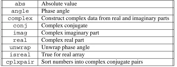
A complete list of the special functions available for handling complex valued quantities is given in table 5.
abs Absolute value
angle Phase angle
complex Construct complex data from real and imaginary parts
conj Complex conjugate
imag Complex imaginary part
real Complex real part
unwrap Unwrap phase angle
isreal True for real array
cplxpair Sort numbers into complex conjugate pairs
Table 5: MATLAB Functions for Complex Valued Quantities
11
The Workspace
If you have been following the above discussion by trying out the above commands for yourself (you should have been), then by now you have quite a few variables defined in what is called your ‘workspace’. To see just which ones are in your workspace, use thewhocommand
Your variables are:
A D ans t y
B F c theta z
C I i x
If you would like to save these variables in such a way as to reload them at some future time, then the following command
>> save archive
will save all these variables into a file namedarchive.mat; any other file name will also do.
Clearing all the variables in your workspace is achieved with theclearcommand, and loading them from a saved file likearchive.matis achieved with theloadcommand:
>> clear >> who
>> load archive >> who
Your variables are:
A D ans t y
B F c theta z
C I i x
One of the most useful and interesting MATLAB commands is the relatedwhycommand, whose operation is really too sophisticated to describe, and hence the reader is urged to try it for themselves.
12
Elementary Plotting
We are now finally at a point where one of the simplest ways in which MATLAB is useful for signals and systems analysis can be illustrated. Specifically, we can show how signals can be constructed and visualized (plotted).
For example, suppose it is necessary to generate and visualise the signal
f(t) = sin(2t), t∈[0,2π].
In this case, the vectortfor the time variable could first be generated as (say) 100 points in the interval
[0,2π]as
>>t = 0:2*pi/99:2*pi;
Note that the increment is2π/99not2π/100since the indexing begins at0, so that such an increment in fact produces 100 points, as can be verified with the command
>> length(t)
ans =
100
Now, generating the signalf(t)is a very simple matter
f = sin(2*t);
>> plot(t,f)
After executing this command, a window should have popped up for you and showing a plot off(t)versus
t.
Notice that the simpler commandplot(f)(try this) will also generate a plot off, but in this case the
xaxis of the plot is the index of the vector element off, whereas with the commandplot(t,f), thet
vector specifies thexaxis.
Your plot can be given a title, as well asxandyaxis labels and a grid as follows (try this for yourself)
>> plot(t,f)
>> xlabel(’time (s)’) >> ylabel(’f’)
>> title(’f(t) versus t’) >> grid on
In fact, this example illustrates another data type in MATLAB - the character string data type. This is nothing more than a vector with elements as ASCII characters rather than real numbers, and it is specified by using quotation characters as in the following example
>> s = ’Expanded Label for Graph: f(t) versus t’; >> s
s =
Expanded Label for Graph: f(t) versus t
>> title(s)
This idea of a character string data type allows us to illustrate a further refinement of the plot function - the specification of the colour, symbol and style of the line used for the plot via a three element string. That is, the plot function can be more fully defined as being of the form
plot(x,y,s)
where
x: Vector of real numbers specifying thexaxis values.
y: Vector of real numbers specifying theyaxis values to be plotted against thexaxis values.
s: Three element character string specifying the plotting line style. The three characters are a
concatena-tion formed as shown in table 6.
Therefore, as examples
>> plot(t,f,’mo-’)
plots magenta circles markers over a solid curve, while
>> plot(t,f,’gd:’)
plots green diamonds over a dotted curve.
The point of these different line-styles is to allow multiple plots on the same set of axes can be discrim-inated. For example, suppose that the function
g(t) = cos(4t)
is to be plotted alongsidef(t), then this can be achieved by
>> g = cos(4*t);
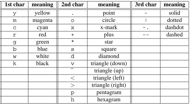
1st char meaning 2nd char meaning 3rd char meaning
y yellow . point - solid
m magenta o circle : dotted
c cyan x x-mark -. dashdot
r red + plus -- dashed
g green * star
b blue s square
w white d diamond
k black v triangle (down)
b triangle (up)
< triangle (left)
> triangle (right)
p pentagram
h hexagram
Table 6: Character codes for line plotting styles
This process of including more items on the same set of axes can be continued indefinitely by adding triples ofx, yaxes and line-style strings:
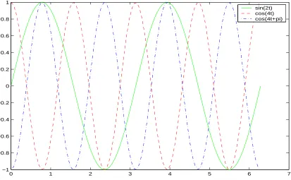
>> h = cos(4*t+pi);
>> plot(t,f,’g-’,t,g,’r--’,t,h,’b-.’)
In order to provide a legend as to which colour and line style corresponds to which plot, this is achieved with thelegendcommand, which accepts a sequence of strings which are labels for the legends, and then associates these strings so that the order of the strings matches the order of the plots. Like so:
>> legend(’sin(2t)’,’cos(4t)’,’cos(4t+pi)’)
If you are trying these commands yourself (you should), then you should see now see something like what is shown in figure 1
13
Script Files
Of course, a necessary convenience for a piece of software such as MATLAB is some means for being able to automate the process of executing commands so that they do not need to be manually typed in every time a particular sequence of them is to be executed.
This convenience is provided by what is known as a script file, and it is very simple. Suppose the following sequence is to be executed
>> t=0:0.01:1; >> f = exp(-5*t); >> plot(t,f)
>> xlabel(’t (s)’) >> ylabel(’exp(-5t)’) >> title(’exp(-5t) vs t’)
Then this sequence could be typed in by hand to the MATLAB prompt as indicated above. On the other hand, one could use an editor (such asnotepadon Windows, oremacson unix) to create a text file calledplotexp.mand then enter the command (without any>>prompt) as
0 1 2 3 4 5 6 7 −1
−0.8 −0.6 −0.4 −0.2 0 0.2 0.4 0.6 0.8 1
sin(2t) cos(4t) cos(4t+pi)
Figure 1: Legend labelled plot of three sinusoidally shaped signals
xlabel(’t (s)’) ylabel(’exp(-5t)’) title(’exp(-5t) vs t’)
This fileplotexp.mis now called a script file, and if it exists in the same directory that MATLAB is currently in (typepwdto see what this directory is, and use thechdircommand to move directory), then the command
>> plotexp
will cause all the commands in the script fileplotexp.mto be run.
Note that the.mfile extension is essential, as it is by this means that MATLAB knows that the function is a script file. On the other hand, the name of the file can be almost arbitrary, except that it must not conflict with the name of another.mfile already known to MATLAB. For example, a name may be used by what is known as a MATLAB ‘toolbox’ routine.
This can be checked with thehelpcommand. For example, suppose that instead ofplotexp.m, the nametryit.mwas to be used as a name. Then first check if this is already being used by
>> help tryit
tryit.m not found.
Clearly, the name is not already being used, so it is fine to use for new purposes.
14
An Alternative to MATLAB
MATLAB is commercial software, so it costs money to obtain and run your own copy. However, there is an alternative calledoctaveavailable as part of thegnuproject which is therefore open-source and costs nothing to download and use. It is available for Windows and Linux platforms from the web site
Notice that this software is not meant to be a clone of MATLAB, and in fact boasts some features not included in MATLAB. However, if it is invoked via the syntax (from, for example, a unix prompt)
% octave --traditional
then it is in a mode whereby its syntax is almost exactly the same as MATLAB. All the examples given in this section will run underoctavewith the syntax given provided it is invoked with the--traditional
option.
The main deficiency ofoctave over MATLAB is not to do with the fundamental structure of the language, but rather to do with the paucity of toolbox’s available foroctavecompared to MATLAB. However, since the material in this book minimises the reliance on add-on MATLAB toolbox functions,