R E S E A R C H
Open Access
A POD-based reduced-order TSCFE
extrapolation iterative format for
two-dimensional heat equations
Zhendong Luo
**Correspondence: [email protected]
School of Mathematics and Physics, North China Electric Power University, No. 2 Bei Nong Road, Beijing, 102206, China
Abstract
In this article, a proper orthogonal decomposition (POD) technique is employed to establish a POD-based reduced-order time-space continuous finite element (TSCFE) extrapolation iterative format for two-dimensional (2D) heat equations, which includes very few degrees of freedom but holds sufficiently high accuracy. The error estimates of the POD-based reduced-order TSCFE solutions and the algorithm implementation of the POD-based reduced-order TSCFE extrapolation iterative format are provided. A numerical example is used to illustrate that the results of the numerical computation are consistent with the theoretical conclusions. Moreover, it is shown that the POD-based reduced-order TSCFE extrapolation iterative format is feasible and efficient for solving 2D heat equations.
MSC: 74S10; 65M15; 35Q35
Keywords: proper orthogonal decomposition technique; reduced-order time-space finite element extrapolation iterative format; two-dimensional heat equations; error estimate
1 Introduction
The time-space finite element (FE) methods for time-dependent partial differential equa-tions (TDPDEs) play an important role in many practical applicaequa-tions and form an impor-tant research topic (see [–]). They have a higher accuracy than their usual FE methods with time-forward difference and even they have a higher accuracy than their Crank-Nicolson FE methods with time-averaged data (see,e.g., [–]). However, even if the time-space continuous finite element (TSCFE) methods for two-dimensional (D) heat equations include a lot of degrees of freedom too, they would cause many difficulties for real-life applications. Therefore, an important problem is how as few it is possible to use to lessen the degrees of freedom so as to alleviate the computational load and save time-consuming calculations and resource demands in the computational process in a way that guarantees the sufficiently accurate numerical solutions.
The proper orthogonal decomposition (POD) method (see []) is an efficient means to lessen the degrees of freedom of numerical models for TDPDEs and alleviate the accu-mulation of truncation errors in the computational process so as to reduce the compu-tational load and save memory requirements. It has been widely and successfully applied to numerous fields, including signal analysis and pattern recognition (see []), statistics,
geophysical fluid dynamics or meteorology (see []). It essentially provides an orthogo-nal basis for representing the given data in a certain least squares optimal sense, namely, it provides a way to find optimal lower dimensional approximations of the given data. Espe-cially, it has played an important role in reduced-order of numerical methods for TDPDEs (see,e.g., [–]). Moreover, the long-term stability of POD reduced-order models is dis-cussed (see,e.g., [–]).
However, almost all existing POD-based reduced-order numerical methods (see,e.g., [–]) employ numerical solutions obtained from classical numerical methods on the total time span [,T] to form POD bases and establish reduced-order models, and then recompute the solutions on the same time span [,T], which actually entails repeating computations on the same time span [,T]. Especially, to the best of our knowledge, there is not any report that the POD-based reduced-order TSCFE extrapolation iterative for-mat for D heat equations is established or that an algorithm of the reduced-order TSCFE extrapolation iterative format is implemented. Therefore, in this article, we establish the POD-based reduced-order TSCFE extrapolation iterative format for D heat equations and provide the error estimates of the POD-based reduced-order TSCFE solutions and the algorithm implementation of the POD-based reduced-order TSCFE extrapolation it-erative format. We also provide a numerical example to illustrate that the POD-based reduced-order TSCFE extrapolation iterative format is feasible and efficient for seeking numerical solutions for D heat equations. Especially, we here thoroughly improve the existing methods, namely, we do only employ the first few given classical TSCFE solu-tions on a very short time span [,T] (TT) as snapshots to form POD basis and establish the POD-based reduced-order TSCFE extrapolation iterative format for seeking the numerical solutions on the total time span [,T]. Thus, we can sufficiently absorb the advantage of the POD method, namely, sufficiently utilize the given data (on very short time span [,T] andTT) to forecast future physical phenomena (on the time span
[T,T]). Therefore, the POD-based reduced-order TSCFE extrapolation iterative format for D heat equations is completely different from the existing POD-based reduced-order methods (see,e.g., [–] etc.) and we have an improvement and development of the existing methods as mentioned above or others.
2 Recall the classical TSCFE method for 2D heat equations and generate snapshots
Let⊂Rbe a bounded and connected polygonal domain. Consider the following D
heat equations (see [, ]).
Problem I Findusuch that
ut–γ u=f, (x,y,t)∈×(,T], (.)
u(x,y,t) = , (x,y,t)∈∂×(,T], (.)
u(x,y, ) =ϕ(x,y), (x,y)∈, (.)
whereut=∂u/∂t,γ is a positive constant, the source termf(x,y,t) and the initial value functionϕ(x,y) are all sufficiently smooth to ensure the following analysis’ validity, and T is the total time.
The Sobolev spaces along with their properties used in this context are standard (see []). For example, define the space
Hm() =
v;
≤|α|≤m
∂x∂α|α∂|vyα
dxdy<∞
,
wherem≥ is integer,α= (α,α),α, andα are two non-negative integers, and|α|=
α+α, with norm
vm=
≤|α|≤m
∂|α|v
∂xα∂yα
dxdy /
and semi-norm
|v|m=
|α|=m
∂x∂α|α∂|vyα
dxdy /
.
Time-space Sobolev spaces are denoted by
Hl ,tn;Hm()
=
v(x,t);
tn
l
i=
di
dtiv(·,t) mdt<∞
with norms
vHl(,tn;Hm)= tn
l
i=
di
dtiv(·,t) mdt
/
.
Especially,vHl(,tn;Hm)are denoted byvHl(Hm)iftn=T.H() ={v∈H();v|∂= }. LetU=H(,T;H
()). Thus, a variational formulation for Problem I is written as
Problem II Seeku(t)∈Usatisfying
(ut,v) +a(u,v) = (f,v), ∀v∈U, (.)
u(x,y, ) =ϕ(x,y), (x,y)∈, (.)
where a(u,v) =γ(∇u,∇v), (·,·) denotes inner product inL(). For the sake of
conve-nience and without loss of generality, we may as well suppose thatγ = in the following theoretical analysis.
In order to establish TSCFE formulation, we first subdivide computational domain into a quasi-uniform triangulationh={K} with h=maxhK, herehK is the diameter
of the triangle K∈ h (see [, , ]), and take the partition on the time span [,T]
as =t<t<· · ·<tN =T with a time stepk=max≤i≤N|ti–ti–|. Then we introduce
the subspaceShm()⊂H() consisting of the piecewise continuousmth degree
poly-nomials defined on the partitionh ofwith mesh parameterh, and letSkl(,T) be an
FE subspace on time partition consisting of continuous piecewiselth degree polynomials, namely,Skl(,T) ={χ∈C([,T]) :χ|
[ti–,ti]∈Pl([ti–,ti])}, wherePl([ti–,ti]) is the set of
polynomials of degree≤lon [ti–,ti]. Finally, we define the time-space element subspace as
Uhk=Shm()⊗Skl(,T).
Thus, the classical TSCFE formulation for the D heat equations is established as follows.
Problem III Finduhk∈Uhksuch that T
uhkt ,φt
+auhk,φt
dt=
T
(f,φt) dt, ∀φ∈Uhk, (.)
uhk(x,y, ) =Phϕ(x,y), (x,y)∈, (.)
wherePh:H
()→Shm() is a Ritz projection, namely, foru∈H(), we have
(∇Phu,∇φ) = (∇u,∇φ), ∀φ∈Shm(). (.)
The TSCFE solutionuhkcan be found by marching through successive time levels. To
this end, letJn= [tn–,tn] andPl(Jn) denote the set of polynomials of degree ≤lon an intervalJn. Then, forn= , , . . . ,N, the TSCFE solutionuhk onJnis found as the unique
solution of
Jn u hk t ,φ
+a uhk,φdt=
Jn
(f,φ) dt, ∀φ∈Shm()⊗Pl–(Jn), (.)
withuhk(x,y, ) =Phϕ
(x,y), anduhk(x,y,tn) (n= , , . . . ,N– , (x,y)∈) are given and
have been found on a previous time step.
In order to improve the accuracy of time approximation,Pl–(Jn) is taken as the set of
end, for eachl≥, consider the Gauss-Legendre integration rule,
g(τ) dτ ∼=
l
j=
wjg(τj), <τ<τ<· · ·<τl< , (.)
which is exact for all polynomials of degree≤l– . For givenl≥, let{i}li= be the
Lagrange polynomials of degreel– corresponding to the points of divisionτ,τ, . . . ,τl,
namely
i(τ) = l
j= j=i
τ–τj
τi–τj
, i= , , . . . ,l. (.)
With the linear transformationt=tn+τkn(kn=tn–tn–) which maps the unit interval [, ] ontoJnand quadrature formula (.), the points of division and weights are denoted by
tn,j=tn+τjkn, n,j(t) =j(τ),
wn,j=
Jn
n,j(t) dt=kn
j(τ) dτ=knwj, j= , , . . . ,l.
(.)
The Lagrange polynomials{ ˜i}li=of degreelcorresponding to the points of division =
τ<τ<τ<· · ·<τl= are denoted by
˜
i(τ) = l
j= j=i
τ–τj
τi–τj
, i= , , . . . ,l. (.)
Puttn,=tn. Note thatun,=uhk(x,y,tn) (n= , , , . . . ,N– ) and ifψ(x,y)∈Shm(),
func-tionϕ=ψ(x,y)n,i(t)∈Shm()⊗Sk(l–)(,T). Thenuhk|Jnis solely determined by the
func-tionsun,j(x,y)≡uhk(x,y,tn,j)∈Shm() such that l
j=
mij un,j,ψ+knwi ∇un,i,∇ψ
=
Jn
n,i f(x,y,t),ψ
dt, i= , , . . . ,l,∀ψ∈Shm(), (.)
uhk(x,y,t) =
l
j=
˜
n,j(t)un,j(x,y), t∈Jn,n= , , . . . ,N, (.)
wheremi,j=Jn˜n,j(t)n,i(t) dt(i= , , . . . ,l;j= , , . . . ,l).
The following results of the existence, the uniqueness, the stability, and the convergence of the solution for the system of equations (.) and (.), namely, Problem III, are ob-tained by means of the same methods as the proofs of Theorems ., ., ., and . in [] or the analogous approaches of proving Theorems ., ., ., and . in [].
Theorem . Ifϕ(x,y)∈H()and f(x,y,t)∈L(,T;L()),there exists a unique solu-tion uhkfor the system of equations(.)and(.),namely,ProblemIIIsatisfying
uhkt L(,tn;H)+∇uhk(x,y,tn)≤C fL(,tn;H–)+∇ϕ
C here and in the following is a constant which is possibly different at different occurrences,
being independent of h and k,but dependent onγ.
()Let u(x,y,t)of the solution to ProblemIIsatisfy u(x,y,t)∈Hm+() (≤t≤T),u∈ Hl+(,T;L()),and u∈H(,T;Hm()).Then we have the following error estimates:
u(x,y,tn) –uhk(x,y,tn)
≤Ckl+uHl+(,tn;H)+hm utL(,tn;Hm)+u(x,y,tn) m+
,
n= , , . . . ,N; (.)
ut(x,y,t) –uhkt (x,y,t)L(,tn;L)
≤Chm+utL(,tn;Hm+)+kl
uHl+(,tn;L)+uHl(,tn;H)
,
n= , , . . . ,N. (.)
() If is convex and the solution u to Problem II is sufficiently smooth that u ∈ Hl+(,T;H()),u∈H(,T;Hm+()),and u(x,y,t)∈Hm+()for each t∈[,T],then we have the following error estimates:
u(x,y,tn) –uhk(x,y,tn)
≤Ckl+uHl+(,tn;H)+hm+u(x,y,tn)
m++uH(,tn;Hm+)
,
n= , , . . . ,N. (.)
Remark . If the source termf(x,y,t), the initial value functionϕ(x,y), the time step k, and the spatial mesh size hall are given, then we can obtain solutionsuhk(x,y,t) by
solving Problem III or the system of equations (.) and (.). But we obtain the first
Msolutionsun,(x,y) =u(x,y,tn) (≤n≤M) (in general,MN, for example,M= , N= ,) by solving (.) atn= , , . . . ,M, which are referred to as snapshots. When one computes actual problems, one may obtain the ensemble of snapshots from physical system trajectories by drawing samples from experiments.
3 Form POD bases and establish POD-based reduced-order TSCFE extrapolation iterative format
In this section, we refer to the idea in [, , , ] to form a POD basis (for more details see [, , , ]) and establish the POD-based reduced-order TSCFE extrapolation iterative format for D heat equations.
Form the matrix A = (Aij)M×M∈RM×M, whereAij= (∇ui,,∇uj,)/Mandun,(x,y) (n=
, , . . . ,M) are the snapshots extracted in Section . Since the matrix A is positive semi-definite with rankκ=dim(span{un,(x,y);n= , , . . . ,M}), its positive eigenvalues and the corresponding orthonormal eigenvectors are used to form POD bases as follows [, , , ].
POD bases is denoted by
ψi(x,y) =
√
Mλi M
j=
vijuj,(x,y), ≤i≤d≤κ. (.)
Furthermore,there is the following error formula:
M M
i= ui,–
d
j=
∇ui,,∇ψjψj
= κ
j=d+
λj. (.)
Let Sdm() =span{ψ,ψ, . . . ,ψd}. For un,(x,y)∈Shm(), define the projection Pd : Shm()→Sdm() as follows:
∇Pdun,,∇wd= ∇un,,wd, ∀wd∈Sdm(). (.)
ThenPdis bounded, that is,
∇Pdun,≤∇un,, ∀un,∈Sdm(). (.)
Thus, by functional analysis theories (see []), there exists an extension Ph : U → L(,T;Shm()) such thatPh|
Shm()=P
d:Shm()→Sdm() defined by
∇Phu,∇wh= (∇u,∇wh), ∀wh∈L ,T;Shm(), (.)
whereu∈U. Due to (.), the projectionPhis also bounded,
∇ Phu≤ ∇u, ∀u∈U. (.)
There is the following inequality (see [, , ]):
u–Phu≤Ch∇ u–Phu, ∀u∈U. (.)
Further, there are the following conclusions (see [, , , ]).
Lemma . For every d(≤d≤κ),the projection Pdsatisfies
M M
i=
ui,–Pdui,+h∇ ui,–Pdui,h ≤Ch
κ
j=d+
λj, (.)
where ui,∈S
hm() (i= , , . . . ,M)are the solutions to (.). Further, if u∈Hr(,T; Hm+())is the solution to ProblemII,then,for all t∈[,T],the projection Ph satisfies the following error estimates:
∂tru(x,y,t) –Phu(x,y,t)s≤Chm+–s∂tru(x,y,t)m+, (.)
where∂r
Thus, based onSdm(), the POD-based reduced-order TSCFE extrapolation iterative format for the D heat equations is established as follows.
Problem IV Findudk∈Sdm()⊗Skl(,T) such that
udk(x,y,t)|Jn= l
j=
˜
n,j(t) d
i=
∇ψi,∇un,j
ψi, n= , , . . . ,M; (.)
l
j=
mij un,jd,ψd
+knwi ∇un,id,ψd
=
Jn
n,i f(x,y,t),ψd
dt, i= , , . . . ,l,∀ψd∈Sdm(), (.)
udk(x,y,t)|Jn= l
j=
˜
n,j(t)un,jd(x,y), n=M+ ,M+ , . . . ,N, (.)
where mi,j=
Jn˜n,j(t)n,i(t) dt (i = , , . . . ,l; j= , , . . . ,l) and un,j (n = , , . . . ,M; j=
, , . . . ,l) are the solutions to (.).
Remark . Ifhis a uniformly regular triangulation, even thoughShm() is the spaces
of piecewise linear polynomials,i.e.,m= , the number of total degrees of freedom for Problem III on each time level isNh×l(whereNh is the number of vertices of triangles inh). Ifm= , the number of total degrees of freedom for Problem III on each time level
is Nh×l, while the number of total degrees of freedom for Problem IV on each time
level isd×l(dκ≤MNNh). For scientific engineering problems, the number Nhof vertices of triangles inhis more than tens of thousands, even more than a hundred
million, whiled is only the number of the first few main eigenvalues so that it is very small (for example, in Section ,d= , whileNh> ×××= ×). Therefore,
Problem IV is the POD-based reduced-order TSCFE extrapolation iterative format with very few degrees of freedom for the D heat equations. Especially, it has no repeating computations and uses the given solutions on the first fewerMtime steps for Problem III to extrapolate other (n–M) solutions, which is completely different from existing reduced-order approaches (see,e.g., [–]etc.).
4 Error analysis and algorithm implementation of POD-based reduced-order TSCFE extrapolation iterative format
4.1 Error estimates of solutions for Problem IV
In the following, we employ classical TSCFE method to derived the error estimates of the POD-based reduced-order TSCFE solutions for Problem IV. We have the following main results for Problem IV.
Theorem . Under the hypotheses of Theorem .,ProblemIVhas a unique solution
udk∈Sdm()⊗Skl(,T)such that
∇udk(tn)≤C fL(,tn;H–)+∇ϕ, n= , , . . . ,M; (.)
uhkt L(,tn;H)+∇uhk(tn)
≤C fL(,tn;H–)+∇ϕ
which show that the solutions to ProblemIVare stable and continuously dependent of the initial value functionϕ(x,y)and the source term f(x,y,t).If M=O(N),then we have the following error estimates between the solution u(t)to ProblemIand the solutions udk to ProblemIV:
u–udk(x,y,tn)
≤Chm+ uH(,tn;Hm+)+u(tn)
m+
+kl+uHl+(,tn;H)
+C
k–/h
κ
i=d+
λj /
, n= , , . . . ,M; (.)
∇ u(tn) –udk(tn)+uhk–udkH(tM,tn;L)
≤Chm utL(,tn;Hm)+u(x,y,tn) m+
+kluHl+(,tn;H)
, n=M+ ,M+ , . . . ,N. (.)
Proof The solutions of Problem IV onJn(n= , , . . . ,M) are obviously unique since they are obtained by projecting the solutions of (.) and (.), namely Problem III on Jn
(n= , , . . . ,M) into POD basis. Moreover, (.) and (.) are immediately obtained from (.)-(.) and Theorem ..
Fort∈Jn(n=M+ ,M+ , . . . ,N), Problem IV has a unique solution by means of the same technique as the proof of Theorem . in [] or the analogous method in []. Equa-tions (.) and (.) are equivalently written as
Jn
udkt ,φdt+a udk,φtddt=
Jn
f,φtddt, ∀φd∈Udkn, (.)
where Un
dk =Sdm()⊗Skl(Jn) (n=M+ ,M+ , . . . ,N) and udk(x,y,tL) =PduL,(x,y) = d
j=(∇ψj,∇uL,)ψj((x,y)∈). By subtracting (.) from Problem III takingφ=φd, we
obtain the following system of error equations:
Jn
uthk–udkt ,φtd+a uhk–udk,φtddt= , ∀φd∈Udkn, (.)
where n =M+ ,M+ , . . . ,N and (uhk –udk)(t
M) = (uhk –Pduhk)(tM) =uM,(x,y) – PduM,(x,y).
Note thatJn= [tn–,tn]. By using the system of error equations (.), (.), and the Hölder
and Cauchy inequalities, we have
uhk–udkH(Jn;L)+ ∇ u
hk–udk(t n)
–
∇ u
hk–udk(t n–)
=
Jn
uhkt –udkt ,uhkt –udkt +a uhk–udk,uhkt –udkt dt
=
Jn
uhkt –udkt ,uhkt –Pduhkt +a uhk–udk,uhkt –Pduhkt dt
+
Jn uhk
t –udkt ,Pduhkt –udkt
+a uhk–udk,Pduhk t –udkt
=
Jn
uhkt –udkt ,uthk–Pduhkt +
d dta u
hk–Pduhk,uhk–Pduhkdt
≤
u
hk–udk H(Jn;L)+
u
hk–Pduhk H(Jn;L)
+ ∇ u
hk–Pduhk(tn) –
∇ u
hk–Pduhk(tn–) .
Note that (uhk–Pduhk)(tM) = (uhk–udk)(tM). By simplifying the above inequality and
sum-ming it fromM+ ton, we obtain
∇ uhk–udk(tn) +u
hk–udk
H(tM,tn;L)
≤∇ uhk–Pduhk(tn)+uhk–PduhkH(tM,tn;L). (.)
Moreover, by Theorem . and Lemma ., we have
∇ uhk–Pduhk(tn)
≤∇ uhk–u(tn)+∇ u–Phu(tn)+∇ Phu–Pduhk(tn)
≤∇ u–Phu(tn)+ ∇ u–uhk(tn)
≤Chm uH(,tn;Hm)+u(x,y,tn) m+
+kl+uHl+(,tn;H)
,
n=M+ ,M+ , . . . ,N; (.)
uhk–PduhkH(tM,tn;L)
≤CkluHl+(,tn;L)+uHl(,tn;H)
+hm+utL(,tn;Hm+)
,
n=M+ ,M+ , . . . ,N. (.)
Combining (.) with (.) and (.) yields
∇ uhk–udk(tn)+uhk–udkH(t
M,tn;L)
≤Chm uH(,tn;Hm)+u(x,y,tn) m+
+kluHl+(,tn;L)+uHl(,tn;H)
, n=M+ ,M+ , . . . ,N. (.)
Combining (.) with Theorem . and (.) yields (.).
With Theorem . and by means of the analogous proof of Theorem ., we easily obtain the following corollary.
Corollary . Under the hypotheses of Theorems . and ., we have the following
L-error estimates for the solutions udkto ProblemIV:
u–udk(x,y,tn)≤C
hm+ uH(,tn;Hm+)+u(tn)
m+
+kl+uHl+(,tn;H)
+C
k–/h
κ
i=d+
λj /
Remark . Due to POD-based reduced-order and extrapolation for the classical TSCFE formulation Problem III, the errors of the solutions for the POD-based reduced-order TSCFE extrapolation iterative format Problem IV include more term (k–/hκ
i=d+λj)/
than those for Problem III, but the degrees of freedom for Problem IV are far less than those of Problem III so that Problem IV can greatly lessen the truncation error accumu-lation in the computational process, alleviate the calculating load, save time-consuming calculations, and improve actual computational accuracy (see the example in Section ). However, the factor (k–/hκ
i=d+λj)/ in Theorem . and Corollary . can act as a
suggestion to choose the number of POD bases, namely, it is only necessary to choosed
such that (k–/hκ
i=d+λj)/=O(kl,hm).
4.2 Algorithm implementation of POD-based reduced-order TSCFE extrapolation iterative format
Finding the solutions of the POD-based reduced-order TSCFE extrapolation iterative for-mat for D heat equations consists of the following six steps.
Step. For given initial value functionϕ(x,y), source termf(x,y,t), and the time step
incrementkand the spatial grid measurementh, solving (.) at the firstMsteps obtains the snapshotsun,(n= , , . . . ,M).
Step. Form the correlation matrix A = (Aij)M×M∈RM×M, whereAij= (∇ui,,∇uj,)/M
and (·,·) isL-inner product.
Step. Let v = (a,a, . . . ,aM)T. Solving the eigenvalue problem Av =λvyields positive
eigenvaluesλ≥λ≥ · · · ≥λκ> (κ=dim(span{un,(x,y);n= , , . . . ,M})) and the corre-sponding eigenvectors vj= (aj
,a j , . . . ,a
j
M)T(j= , , . . . ,κ).
Step. For the errorδ=O(kl,hm) needed, determine the numberdof POD basis such
thatk–/hκ
j=d+λj≤δ.
Step . Generate POD basisψi= M
j=aijuj,(x,y)/
√
Mλi (j= , , . . . ,d). Let Sdm() = span{ψ,ψ, . . . ,ψd}. Solving Problem IV withddegrees of freedom obtainsudk(x,y,t).
Step. If∇(un–,d –udn,)≥ ∇(un,d –u n+,
d ) (n=M,M+ , . . . ,N– ), thenudk
are the solutions for Problem IV satisfying accuracy needed. Else, namely, if∇(un–,d –
un,d )<∇(un,d –u n+,
d )(n=M,M+ , . . . ,N– ), letui,=un–M–i(i= , , . . . ,M) and
return toStep.
5 A numerical example
In this section, we present a numerical example showing the advantage of the POD-based reduced-order TSCFE extrapolation iterative format for D heat equations.
Its computational domain is irregular and consists of a set = ([, ] × [, ])∪ ([, .]×[., .]) cm. The triangularization
hfor computational domainadopts
local refining meshes such that the scale of meshes on [, .]×[., .] and nearby (,y) (≤y≤) are one third of meshes nearby (,y) (≤y≤). Buth=√×–, whose
nodesNh> ×. We take the time step increment ask= – s (second). Subspaces Shm() andSkl(,T) are taken as piecewise second polynomial spaces, namely,m= and l= , respectively. The source term is taken asf(x,y,t) = , the initial and boundary valve functions are taken as follows, for ≤t≤T:
ϕ(x,y) = ⎧ ⎪ ⎨ ⎪ ⎩
ϕ(x,y) = , and the boundary value function as follows:
ϕ(x,y,t) =
ϕ(x,y), (x,y)∈∂,t= , un–
h (x,y,t), (x,y)∈∂,t=tn,n= , , . . . ,n.
We first take the firstM= solutionsun,(x,y) =u(x,y,tn) for the classical TSCFE for-mulation, namely, Problem III at time partition pointstn(n= , , . . . , ) as snapshots. Then we find the eigenvalues λ ≥λ ≥ · · · ≥λ≥ and the corresponding
eigen-vectors vj= (aj,aj, . . . ,aj )T (j= , , . . . , ) for the matrix A = (Aij)×, whereAij=
(∇ui,,∇uj,)/. It is shown by computing that error factor (k–/h
i=λj)/≤×–.
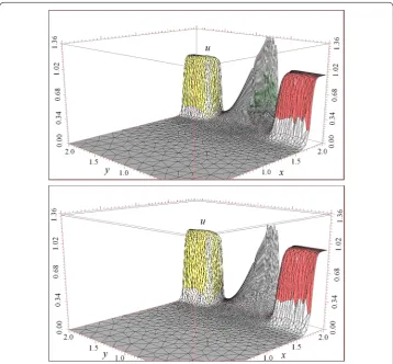
Thus, it is only necessary to take the most main six POD bases. According to steps in Section . without renewing POD basis, the POD-based reduced-order TSCFE extrapo-lation iterative format are still convergent, whose solution att= is found and depicted on the top chart in Figure . The numerical solutionun
hobtained with classical Problem III
whenn= , (i.e.,t= ) is depicted graphically on the bottom chart in Figure . The two charts in Figure exhibit a quasi-identical similarity. Although the errors of the POD-based reduced-order TSCFE solutions on the starting time span are slightly larger than those of the classical TSCFE solutions, since the POD-based reduced-order TSCFE
ex-Figure 1 Classical TSCFE solutionsun
dand the reduced-order TSCFE solutionu n
d.The top chart is the reduced-order TSCFE solutionun
dwhend= 6 atn= 1,000 (t= 10). The bottom chart is the classical TSCFE
solutionun
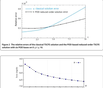
Figure 2 The relative errors of the classical TSCFE solution and the POD-based reduced-order TSCFE solution with six POD bases on 0≤t≤10.
Figure 3 The error (log 10) chart between the classical TSCFE solution and the POD-based reduced-order TSCFE solutions with different number of 20 POD bases att= 10.
trapolation iterative format Problem IV on each time level only includes × degrees of freedom and the classical TSCFE formulation Problem III has more than ××
degrees of freedom, namely, the degrees of freedom for the POD-based reduced-order TSCFE extrapolation iterative format are far fewer than those for the classical TSCFE for-mulation Problem III so that it could greatly lessen the truncation error accufor-mulation in the computational process, alleviate the calculating load, save the consuming time of calculations, and improve the actual computational accuracy; therefore, after some time span, the numerical errors of the POD-based reduced-order TSCFE extrapolation itera-tive format are fewer than those of the classical TSCFE formulation (see Figure ).
Figure shows the errors between solutions obtained from the POD-based reduced-order TSCFE extrapolation iterative format with different number of POD bases and solu-tions obtained from the classical TSCFE formulation att= . It is shown that the numer-ical computing results are consistent with those obtained for the theoretnumer-ical case because the theoretical and numerical errors are allO(–).
Further, by comparing the classical TSCFE formulation with the POD-based reduced-order TSCFE extrapolation iterative format with six POD bases implementing the numer-ical simulations att= , it is found that the classical TSCFE formulation includes more than ××unknown quantities (since the subspacesShm() andSkl(,T) are taken
format with six POD bases does only include six unknown quantities on each time level and the corresponding computing time is less than seconds, namely, the computing time of the classical TSCFE formulation is times higher than that of the POD-based reduced-order TSCFE extrapolation iterative format with six POD bases. Thus, the POD-based reduced-order TSCFE extrapolation iterative format can greatly save the calculating time and alleviate the computing load so that it could greatly lessen the truncation error accumulation in the computational process. It is also shown that finding the numerical solutions for D heat equations by means of the POD-based reduced-order TSCFE ex-trapolation iterative format is computationally very effective and feasible.
6 Conclusions and discussions
In this article, the POD-based reduced-order TSCFE extrapolation iterative format for D heat equations has been established, the error estimates of the POD-based order TSCFE solutions and the algorithm implementation of the POD-based reduced-order TSCFE extrapolation iterative format have been provided. A numerical example has been used to validate that the results of the numerical computation are consistent with the theoretical conclusions. Further, it has shown that the POD-based reduced-order TSCFE extrapolation iterative format can greatly save the calculating time and alleviate the computing load so that it could greatly lessen the truncation error accumulation in the computational process. Moreover, it is shown that the POD-based reduced-order TSCFE extrapolation iterative format is computationally very effective and feasible for finding the numerical solutions to D heat equations.
Though some POD-based reduced-order models for D parabolic equations have been established (see [, , , , ]), the POD-based reduced-order TSCFE extrapolation iterative format here is completely different from those mentioned above because the TSCFE method is different from the usual Galerkin method, the FE method, the finite vol-ume method, and the finite difference scheme. Especially, the POD-based reduced-order TSCFE extrapolation iterative format only employs the first few given classical TSCFE so-lutions on the very short time span [,T] (TT) as snapshots to form the POD basis and seek the numerical solutions on the total time span [,T]. It is an improvement and innovation of the existing methods (see,e.g., [–]etc.).
Future research work in this area will aim to extend the POD-based reduced-order TSCFE extrapolation iterative format, applying it to more TDPDEs such as the nonlin-ear Schrödinger equation, integral differential equations, convection-diffusion equations, nonlinear sine-Gordon equation, Sobolev equations, solute transport equations, and vis-coelastic equations.
Competing interests
The author declares that he has no competing interests.
Acknowledgements
This research was supported by National Science Foundation of China grant 11271127 and Science Research Project of Guizhou Province Education Department grant QJHKYZ[2013]207.
Received: 19 October 2014 Accepted: 23 March 2015
References
1. Aziz, AK, Monk, P: Continuous finite elements in space and time for the heat equation. Math. Comput.52, 255-274 (1989)
3. Li, H, Liu, RX: The space-time finite element method for parabolic problems. Appl. Math. Mech.22(6), 687-700 (2001) 4. Bales, L, Lasiecka, I: Continuous finite elements in space and time for the nonhomogeneous wave equation. Comput.
Math. Appl.27(3), 91-102 (1994)
5. French, DA, Peterson, TE: A continuous space-time finite element method for the wave equation. Math. Comput.
65(214), 491-506 (1996)
6. Liu, Y, Li, H, He, S: Mixed time discontinuous space-time finite element method for convection diffusion equations. Appl. Math. Mech.29(12), 1579-1586 (2008)
7. French, DA: A space-time finite element method for the wave equation. Comput. Methods Appl. Mech. Eng.107, 145-157 (1993)
8. Luo, ZD: The Foundations and Applications of Mixed Finite Element Methods. Chinese Science Press, Beijing (2006) (in Chinese)
9. Thomée, V: Galerkin Finite Element Methods for Parabolic Problems, 2nd edn. Springer, Berlin (2003)
10. Thomée, V: Negative norm estimates and superconvergence in Galerkin methods for parabolic problems. Math. Comput.34, 93-113 (1980)
11. Holmes, P, Lumley, JL, Berkooz, G: Turbulence, Coherent Structures, Dynamical Systems and Symmetry. Cambridge University Press, Cambridge (1996)
12. Fukunaga, K: Introduction to Statistical Recognition. Academic Press, New York (1990) 13. Jolliffe, IT: Principal Component Analysis. Springer, Berlin (2002)
14. Ly, HV, Tran, HT: Proper orthogonal decomposition for flow calculations and optimal control in a horizontal CVD reactor. Q. Appl. Math.60, 631-656 (2002)
15. Kunisch, K, Volkwein, S: Galerkin proper orthogonal decomposition methods for parabolic problems. Numer. Math.
90, 117-148 (2001)
16. Kunisch, K, Volkwein, S: Galerkin proper orthogonal decomposition methods for a general equation in fluid dynamics. SIAM J. Numer. Anal.40, 492-515 (2002)
17. Kunisch, K, Volkwein, S: Control of Burgers’ equation by a reduced order approach using proper orthogonal decomposition. J. Optim. Theory Appl.102, 345-371 (1999)
18. Ahlman, D, Södelundon, F, Jackson, J, Kurdila, A, Shyy, W: Proper orthogonal decomposition for time-dependent lid-driven cavity flows. Numer. Heat Transf., Part B, Fundam.42, 285-306 (2002)
19. Luo, ZD, Chen, J, Xie, ZH, An, J, Sun, P: A reduced second-order time accurate finite element formulation based on POD for parabolic equations. Sci. Sin., Math.41(5), 447-460 (2011) (in Chinese)
20. Luo, ZD, Li, H, Zhou, YJ, Huang, XM: A reduced FVE formulation based on POD method and error analysis for two-dimensional viscoelastic problem. J. Math. Anal. Appl.385, 371-383 (2012)
21. Luo, ZD, Li, H, Zhou, YJ, Xie, ZH: A reduced finite element formulation and error estimates based on POD method for two-dimensional solute transport problems. J. Math. Anal. Appl.385, 371-383 (2012)
22. Luo, ZD, Du, J, Xie, ZH, Guo, Y: A reduced stabilized mixed finite element formulation based on proper orthogonal decomposition for the non-stationary Navier-Stokes equations. Int. J. Numer. Methods Eng.88(1), 31-46 (2011) 23. Luo, ZD, Xie, ZH, Shang, YQ, Chen, J: A reduced finite volume element formulation and numerical simulations based
on POD for parabolic equations. J. Comput. Appl. Math.235(8), 2098-2111 (2011)
24. Luo, ZD, Xie, ZH, Chen, J: A reduced MFE formulation based on POD for the non-stationary conduction-convection problems. Acta Math. Sci.31(5), 1765-1785 (2011)
25. Li, HR, Luo, ZD, Chen, J: Numerical simulation based on proper orthogonal decomposition for two-dimensional solute transport problems. Appl. Math. Model.35(5), 2489-2498 (2011)
26. Luo, ZD, Zhou, YJ, Yang, XZ: A reduced finite element formulation based on proper orthogonal decomposition for Burgers equation. Appl. Numer. Math.59(8), 1933-1946 (2009)
27. Luo, ZD, Chen, J, Sun, P, Yang, XZ: Finite element formulation based on proper orthogonal decomposition for parabolic equations. Sci. Sin., Math.52(3), 587-596 (2009)
28. Luo, ZD, Chen, J, Navon, IM, Yang, XZ: Mixed finite element formulation and error estimates based on proper orthogonal decomposition for the non-stationary Navier-Stokes equations. SIAM J. Numer. Anal.47(1), 1-19 (2008) 29. Luo, ZD, Chen, J, Navon, IM, Zhu, J: An optimizing reduced PLSMFE formulation for non-stationary
conduction-convection problems. Int. J. Numer. Methods Fluids60(4), 409-436 (2009)
30. Luo, ZD, Zhu, J, Wang, RW, Navon, IM: Proper orthogonal decomposition approach and error estimation of mixed finite element methods for the tropical Pacific Ocean reduced gravity model. Comput. Methods Appl. Mech. Eng.
196(41-44), 4184-4195 (2007)
31. Luo, ZD, Li, H, Shang, YQ, Fang, Z: A LSMFE formulation based on proper orthogonal decomposition for parabolic equations. Finite Elem. Anal. Des.60, 1-12 (2012)
32. Bergmann, M, Bruneau, CH, Iollo, A: Enablers for robust POD models. J. Comput. Phys.228(2), 516-538 (2009) 33. Deane, AE, Kevrekidis, IG, Karniadakis, GE, Orsag, SA: Low-dimensional models for complex geometry flows:
application to grooved channels and circular cylinder. Phys. Fluids A3(10), 2337-2354 (1991)
34. Ma, X, Karniadakis, GE: A low-dimensional model for simulating three-dimensional cylinder flow. J. Fluid Mech.458, 181-190 (2002)
35. Wang, Z, Akhtar, I, Borggaard, J, Iliescu, T: Two-level discretizations of non-linear closure models for proper orthogonal decomposition. J. Comput. Phys.230, 126-146 (2011)
36. Adams, RA: Sobolev Spaces. Academic Press, New York (1975)