Cross-diffusion-driven Turing instability and weakly nonlinear analysis of Turing patterns in a uni-directional consumer-resource system

R E S E A R C H

Open Access

Cross-diffusion-driven Turing instability

and weakly nonlinear analysis of Turing

patterns in a uni-directional

consumer-resource system

Renji Han

_{and Binxiang Dai}

*_{Correspondence:}

[email protected]

1_{School of Mathematics and}

Statistics, Central South University, Changsha, 410083, China Full list of author information is available at the end of the article

Abstract

Spatiotemporal patterns driven by cross-diffusion of a uni-directional consumer-resource (C-R) system with Holling-II type functional response are investigated in this paper. The existence of a unique positive steady state of the considered system is studied first. The linear stability analysis shows that the cross-diffusion is the key mechanism for the formation of spatiotemporal patterns through Turing bifurcation. We choose the cross-diffusion coefficient as bifurcation parameter and discuss three different types of Turing bifurcations, corresponding to simple, double non-resonant and double resonant cases. Based on weakly nonlinear analysis with the multiple scale method and the adjoint system theory, we derive the amplitude equations of the Turing patterns near the Turing bifurcation point and obtain the analytical approximation solutions of the patterns for each case. Specially, some qualitative results of amplitude equations of the resonant case are given in detail. Finally, numerical simulations are performed to illustrate the weakly nonlinear theoretical predictions and through these simulations some patterns (single mode pattern, mixed-mode pattern, super-squares pattern, roll pattern, hexagonal pattern) are found. Simultaneously, numerical simulations show that the resource supplying rate has an important impact on the direction of Turing bifurcation.

MSC: 35B32; 35B36; 35K57; 92D25; 92D40

Keywords: cross-diffusion; uni-directional C-R system; Turing pattern; amplitude equation; weakly nonlinear analysis

1 Introduction

The interaction of populations is one of the basic interspecies relations in biology and ecol-ogy []. The consumer-resource (C-R) system was originally incorporated into the study of interspecies interactions to describe the mechanisms or ways by which individuals of different species interact with one another []. A resource is considered to be a biotic or abiotic species that increases the population growth of its consumers, whereas a consumer exploits a resource and then reduces its growth rate. In this way, species interactions clude bi-directional, uni-directional, and indirect C-R interactions. Bi-directional C-R in-teractions occur when each species functions as both a consumer and a resource of the

other. Uni-directional C-R interactions occur when one species functions as a consumer and the other as a material and/or energy resource, but neither acts as both. Indirect C-R interactions occur when the effects of the two species on one another are mediated en-tirely by the density or traits of a third species that is a consumer or resource of one or both of them []. The general model of uni-directional C-R interactions proposed by Holland and DeAngelis [] is

⎧ ⎨ ⎩

du

dt =u[r+ef(u,v) –qg(u,v) –du], dv

dt =v[r+ef(u,v) –dv],

(.)

whereurepresents the population density of the resource, andvrepresents the population density of the consumer.randrare intrinsic growth rates in the absence of the other

species. The ratiosr/dandr/dcan be thought of as carrying capacities in the absence of

the other species. The termeifi(u,v) represents the gain from the interaction, and the term

qg(u,v) represents the costs incurred by the interaction. In this case, there are positive

effects occurring to both populations, but the speciesuhas only one that incurs a loss due to the C-R interaction. In the uni-directional C-R interaction, the consumer provisions the resource species with a non-trophic beneficial service of dispersal or defense in the other direction []. As an example, consider an interaction between an insect pollinator species and the host plant species. The pollinator both pollinates the plant’s flowers and oviposits on them, so that the insect’s larvae can feed on the plant’s seeds.

Since the pioneering work of Holland and DeAngelis [, ], some articles on C-R interac-tion models have been published to illustrate the importance of this interacinterac-tion. Previous studies of C-R interaction models mainly focused on the mechanisms that determine how interaction outcomes depend on the model parameters. Gross [] considered positive in-teractions among competitors in two kinds of resource-competition models. Wanget al. [] used uni-directional C-R theory to investigate the transitions of interaction outcomes for a kind of uni-directional C-R system. Based on the model (.), Wang and DeAngelis [] considered a specific uni-directional C-R system as follows:

⎧ ⎨ ⎩

du

dt =u[r+

αv

c+v–βv–du], dv

dt =v[r+

αu c+u–dv],

(.)

whereu,v,rianddihave the same meanings as those in the general model (.), and the

meanings of the other parameters in the system are referred to in Table . They studied the dynamical behavior of the system and demonstrated in this mechanism how and when interaction outcomes of this system vary with different conditions.

Table 1 Parameter definitions in systems (1.2)-(1.3) and their units, where [speciesu] indicates the speciesudensity and [speciesv] indicates speciesvdensity

Symbol Parameter definition Units

r1 Speciesuintrinsic growth rate 1/time

r2 Speciesvintrinsic growth rate 1/time

c1 Half-saturation density constant of speciesu [speciesu]

c2 Half-saturation density constant of speciesv [speciesv]

α12 Resource consumption rate of speciesu 1/time

β1 Resource supplying rate of speciesu [speciesv]–1_(1/time)

α21 Resource consumption rate of speciesv 1/time

r1/d1 Speciesucarrying capacity [speciesu]

r2/d2 Speciesvcarrying capacity [speciesv]

a1 Self-diffusion coefficient of speciesu (distance)2(1/time)

a2 Self-diffusion coefficient of speciesv (distance)2(1/time)

b Cross-diffusion coefficient of speciesv (distance)2_{(1/time)[speciesu]}–1

the individuals escape from high infection risks and so on (for example, see [–] and references therein). Considering the effects of spatial diffusion, Huanget al.[] studied bifurcation and temporal periodic patterns in a delayed plant-pollinator model with a dif-fusion effect.

More generally, there exists a motional state of interaction as well, one that recognizes the possible bias, say, of the motion of one species toward or away from another species [, ]. This phenomenon is called cross-diffusion. The value of the cross-diffusion coef-ficient can be positive or negative. The term including positive cross-diffusion coefficients denotes the movement of the species in the direction of lower concentration of another species and negative cross-diffusion coefficients denote that one species tends to diffuse in the direction of a higher concentration. Since the pioneer work of [], the concern on cross-diffusion in ecological models has attracted the attention of biologists, chemical experimenters and applied mathematicians and cross-diffusion has been one of the dom-inant topics in both ecology and mathematical ecology because of its universal existence and importance ([, ]). Shigesadaet al.[] investigated the effect of cross-diffusion in a competitive population system first. Then, many works have proposed to investigate the Turing instability driven by cross-diffusion and prove the existence of inhomogeneous steady states that induce the emergence of spatial patterns ([–] and [–]). Hence it is of great interest to explore the role of cross-diffusion in driving Turing instability and spatial pattern formation.

Based on the statements above, in this paper, we introduce the spatial diffusion with zero-flux boundary conditions into system (.), and further assume that speciesuis sub-ject to self-diffusion, and that speciesvis subject to nonlinear positive cross-diffusion. We examine how the cross-diffusion induces the Turing instability and the spatial inhomoge-neous distribution of the two species. Then the considered system appears as follows:

⎧ ⎪ ⎪ ⎪ ⎪ ⎪ ⎨ ⎪ ⎪ ⎪ ⎪ ⎪ ⎩

∂u(x,y,t)

∂t =a∇ _u+f

(u,v), (x,y)∈,t> ,

∂v(x,y,t)

∂t =∇ · ∇((a+bu)v) +f(u,v), (x,y)∈,t> ,

∂u(x,y,t)

∂ν = ∂v(x,y,t)

∂ν = , (x,y)∈∂,t> , u(x,y, ) =u(x,y), v(x,y, ) =v(x,y), (x,y)∈,

with

f(u,v) =u

r+

αv

c+v

–βv–du

,

f(u,v) =v

r+

αu

c+u

–dv

.

Hereu(x,y,t) andv(x,y,t) represent the numbers of biomass density of the two species at any instant of timetand location (x,y) subject to the non-negative initial conditionu(x,y)

andv(x,y) and Neumann boundary conditions∂u/∂ν=∂v/∂ν= ;∇is the gradient

op-erator in domainandνis the outward unit normal vector on∂. The homogeneous Neumann boundary conditions reflect the situation where the population cannot cross the boundary of.is a bounded open domain inR with smooth boundary∂. The parametersa,aare the positive self-diffusion coefficients whilebis the cross-diffusion

coefficient. The meanings of other parameters in system (.) are the same as in system (.). Referring to [], the units of parameters of system (.) are summarized in Table . In our current work we first investigate the effect of cross-diffusion on the spatial inho-mogeneous distribution of the two species in a uni-directional C-R system. Our results show that the resource supply rate has an important effect on the Turing bifurcation di-rection. We also show how the weakly nonlinear analysis of the C-R system (.) is able to point out some interesting phenomena like stable supercritical and subcritical Turing patterns and a hysteretic-type phenomenology due to the presence of a multiplicity of real stable equilibria for the amplitude equation in the subcritical case. The rest of the paper is organized as follows. Section  discusses the existence and unique positive spatially homo-geneous steady state of system (.). The linear stability analysis of the proposed system and its corresponding non-spatial system are presented in Section . Weakly nonlinear pattern analysis and the related numerical simulations are given in Section . A brief con-clusion and discussion are presented in Section . In the Appendix, we give the coefficient expressions of amplitude equations emerged in Section .

2 Existence of unique positive spatially homogeneous steady state

In this section, we shall prove the existence and uniqueness of a positive spatially homoge-neous steady state for system (.) by analytical methods. Clearly system (.) admits one trivial steady state:E:= (, ) and two semi-trivial constant steady states:E:= (_dr_, )

andE:= (,_dr_). In biology, we are interested in positive spatially homogeneous steady

states. System (.) admits a positive spatially homogeneous steady stateE∗:= (u∗,v∗) ifE∗

is a positive constant solution to the following two equations:

r+

αv

c+v

–βv–du= , (.)

r+

αu

c+u

–dv= . (.)

Assume that

(H): _dr_ <

r+α–cβ+

√

(r+α–cβ)+rβc

β .

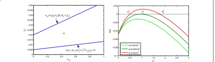
Figure 1 Graphs ofG1(v) andG2(v).Figure 1

depicts that there exist parameters such that system (1.3) has a unique positive steady state. Here the parameter values of system (1.3) are chosen as r1= 0.6,r2= 0.3,α12= 0.1,α21= 0.3,c1=c2= 0.1,

d1=d2= 0.01,β1= 0.01. A direct calculation yields

the unique positive steady state (u_∗,v_∗) = (10.2725, 59.7108).

Theorem . Under(H),system(.)has a unique positive spatially homogeneous steady

state E∗.

Proof It follows from (.) that  <v<r+α d . Define

F(v) =

 d

r+

αv

c+v

–βv

, F(v) =

cα

r+α–dv

–c,

forv∈(,r+α

d ). From (.) and (.), we know that the zero isoclines of system (.) are

given byu=F(v) andu=F(v), respectively. Then the positive spatially homogeneous

steady stateE∗= (u∗,v∗) of system (.) should satisfyu∗=F(v∗) =F(v∗). Thus the

ques-tion to look for a positive spatially homogeneous steady state is reduced to finding a pos-itive constant solutionvsuch thatF(v) =F(v). A direct calculation yields

F() =

r

d

, F

v = , F_(v) =  d

–β+

αc

(c+v)

,

F_(v) = – αc d(c+v)

< ,

and

F

r

d

= , F_(v) = cαd (r+α–dv)

> , F_(v) = cαd

 

(r+α–dv)

> .

Denote by (,v) the intersection of the zero isoclineu=F(v) and the v-axis. Then

we getv₌r+α–bβ+

√

(r+α–bβ)+rβb

β . From the equalities above, we see thatu=

F(v) is a continuous concave function on (,v) satisfyingF() =_dr_ >  andF(v) = .

Letuˆ=F(vˆ) =_d_(r+α_c₊v_vˆ_ˆ_ –βvˆ),vˆ=

_α

c

β –c. Since dF

dv|v=vˆ=  andF(v) < ,

(uˆ,vˆ) is the maximum point of the functionu=F(v) andF(v) is concave left as shown

in Figure . Hence, whenv<vˆ,u=F(v) is monotonically increasing; whenv>vˆ,u=F(v)

is monotonically decreasing.

It is clear that u=F(v) is a continuous and increasing concave down function on

(,r+α

d ) satisfyingF() = –cr

r+α < ,F( r

d) =  andlimv→r+dα–

F(v) = +∞.

Combining the above analysis and (H), we see that there is a unique constant

solu-tionv∗∈(,v) such thatu∗=F(v∗) =F(v∗) and is positive. Therefore, system (.) has

a unique positive spatially homogeneous steady state E∗ = (u∗,v∗). This completes the

proof.

3 Stability analysis

are interested in investigating the Turing instability of the system (.), which is induced by cross-diffusion, that is, the positive steady stateE∗of the model without cross-diffusion

is stable, but it is unstable in the presence of the cross-diffusion termbuv.

3.1 Stability analysis of the corresponding ODE system

First, we perform the stability analysis of the positive spatially homogeneous steady state E∗in the absence of diffusion, that is, the system (.) degenerates to the corresponding ordinary differential equation (ODE) system (.) in this case. To study this, we linearize the system (.) along the positive steady stateE∗and the linear stability is determined by

the eigenvalues of the following Jacobian matrix:

K=

K K

K K

, (.)

where

K= –du∗, K=

αcu∗

(c+v∗)

–βu∗, K=

αcv∗

(c+u∗)

, K= –dv∗.

The corresponding characteristic equation ofKis

λ–tr(K)λ+det(K) = , (.)

where

tr(K) =K+K, det(K) =KK–KK.

Theorem . Assume that(H)holds.Then we have

(i) System(.)cannot undergo a Hopf bifurcation at the positive spatially homogeneous

steady stateE∗.

(ii) Furthermore,if the parameters of the system(.)satisfy

(du∗–βv∗)(c+v∗)+αcv∗< , (.)

then the positive spatially homogeneous steady stateE∗is locally asymptotically stable.

Proof Sincetr(K) <  always holds, there is not any pair of imaginary roots in the charac-teristic equation (.), and the proof of (i) is completed.

(ii) Noting that

det(K) =ddu∗v∗–

αcv∗

(c+u∗)

αcu∗

(c+v∗) –βu∗

=ddu∗v∗+ αcu∗

(c+u∗)

βv∗– αcv∗

(c+v∗)

,

it follows from the assumption (.) thatdet(K) > . Clearlytr(K) = –du∗–dv∗< . Thus

is locally asymptotically stable in the absence of self-diffusion and cross-diffusion. This

completes the proof of the theorem.

3.2 No Turing instability without cross-diffusion

In this subsection, we shall prove system (.) still remains stable in the presence of self-diffusion but without cross-self-diffusion (i.e.,b= ). Then the linearized form of system (.) withb=  along the unique positive spatially homogeneous steady stateE∗= (u∗,v∗) can

be written as follows:

˙

w=Kw+

a 

 a

∇_{w, w=}

u–u∗

v–v∗

, (.)

withKgiven by (.).

Let us consider the solution of system (.) in the form

w=

c_k c k

eλt+ik·r, (.)

where k = (kx,ky), k·k=k,λis the growth rate of perturbation in timet,kxandky

repre-sent the wave numbers of the solutions, i is the imaginary unit, i_{= – and r = (x,y) is the}

spatial vector in two-dimensional space. Substituting (.) into (.) leads to the following dispersion relation, which gives the eigenvalueξas a function of the wave numberk=|k|:

λ–Trkλ+ k= , (.)

where

Trk=tr(K) –k(a+a), k=aak+ (adv∗+adu∗)k+det(K). (.)

The following theorem shows that Turing instability does not occur in the uni-directional C-R system (.) without cross-diffusion.

Theorem . Assume that(H), (.)and b= in system(.).Then the unique positive

spatially homogeneous steady state E∗= (u∗,v∗)is locally asymptotically stable.

Proof Since the assumption (.) holds, we getdet(K) > . Clearlytr(K) < . ThusTrk< 

and k> . This completes the proof.

3.3 Turing instability induced by cross-diffusion

In this subsection, we shall prove that the only potential destabilizing mechanism in our system (.) is the presence of the cross-diffusion. Linearizing system (.) along the pos-itive steady stateE∗= (u∗,v∗) yields

˙

w=Kw+Db∇w, w=

u–u∗

v–v∗

, (.)

whereDb₌a 

Substituting (.) into (.) leads to the following dispersion relation, which gives the eigenvalueλas a function of the wave numberk=|k|:

λ+gk λ+hk = , (.)

where

gk =ktrDb –tr(K), hk =detDb k+qk+det(K), (.)

and

q=adv∗+adu∗+bu∗

du∗–βv∗+

αcv∗

(c+v∗)

. (.)

Theorem . (Cross-diffusion induced Turing instability) Assume that (H) and(.)

hold.Then the unique positive spatially homogeneous steady state E∗(u∗,v∗)of system(.)

is spatially unstable when b>bc,and the critical wave number is given by k_c,where bcand k

c can be found in the proof of the theorem.

Proof From Theorem . and Theorem ., we know that system (.) still remains stable without diffusion or in the presence of self-diffusion alone. Therefore, it follows that the only potential destabilizing mechanism is the presence of the cross-diffusion terms. Then for the Turing instability to be realized and spatial patterns to form, there must be some k=  such that the real part of at least one root of the characteristic equation (.) is greater than zero. Sinceg(k_{) >  for∀k= , instability can only be obtained in the case of}

h(k_{) <  for somek= . Sincedet(D}b_{) > , we get the condition for the marginal stability}

as follows:

minhk =hk_m = , (.)

where

k_m = – q

det(Db₎, (.)

which requires that q< . Fromq< , we know that the necessary condition of Turing instability is as follows:

du∗–βv∗+

αcv∗

(c+v∗) < , (.)

which is equivalent to the assumption (.).

In what follows, we shall choose the cross-diffusion coefficientbas bifurcation param-eter. Let us now setq= –γb+δ, where the positive quantitiesγ andδare defined as:

γ = –u∗

du∗–βv∗+

αcv∗

(c+v∗)

Letb=_γδ +η. At bifurcation,min(h(k_{)) = . Then substitutingbinto the second equality}

of (.) yields the following equation forη:

γη

det(K)–au∗η–

aa+au∗

δ γ

= . (.)

Clearly, equation (.) has a unique positive root. Denote the unique positive root of equation (.) byη+_{. Set}

bc= δ γ +η

+_{. (.)}

Since

q=  ⇔ b∗= δ γ,

we can see that  <b∗<bc_{andq< ,min(h(k}_{)) <  whenb>b}c_{. Therefore, the unique}

steady stateE∗is unstable. This indicates that a Turing instability occurs and the critical value for bifurcation isb=bc_{. The critical wave numberk}

cis then given (using (.)) by

k_c= γ η

+

det(Dbc

). (.)

This completes the proof.

Remark  Whenb>bc, there exists a range (k_,k_) of unstable wave numbersksuch that h(k_{) < , and correspondingly the real part of the eigenvalue of equation (.)Re(λ) > ;}

see on the right of Figure .

In what follows, we shall consider only the case where there is one unstable eigenvalue, admissible for the Neumann boundary conditions, which falls within the band (k_,k_) in the sense ofk

 <k=φ+ψ<kwithφ=l

π

Lx andψ = nπ

Ly, wherel,nare integers. We

denote bykˆ

c the unstable admissible eigenvalue to distinguish it from the critical valuekc.

As an example, we take the parameters of system (.) asr= .,r= .,c=c= .,

Figure 2 Left: the growth rateα12vs. the consumption rateβ1; Right: dispersion relation.In Figure 2, the bounded areashows the parameter space where Turning instability may occur and the parameter values are chosen asr1= 0.6,r2= 0.3,α21= 0.3,c1=c2= 0.1,d1=d2= 0.01. To the right of the figure, the

parameter values are chosen asr1= 0.6,r2= 0.3,c1=c2= 0.1,d1=d2= 0.01,α21= 0.3,α12= 0.6,β1= 0.02,

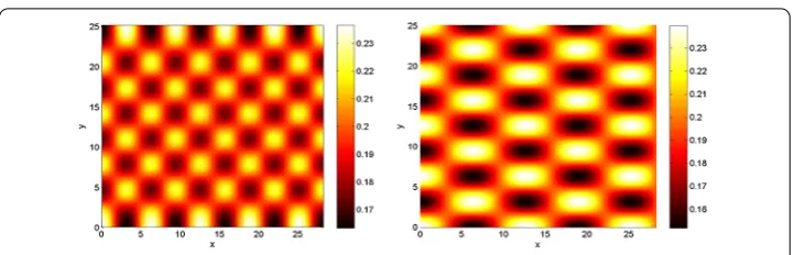
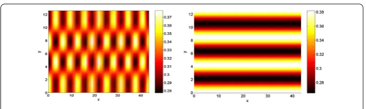
Figure 3 Snapshots of contour picture of spatial distribution of the speciesu(left) and speciesv

(right).Figure 3 depicts the pattern formation of the two species when the cross-diffusion coefficientbis greater than its critical valuebc_{. The parameters of system (1.3) are chosen asr}

1= 0.6,r2= 0.3,c1=c2= 0.1,

d1=d2= 0.01,α12= 0.4,β1= 0.02,α21= 0.3,a1= 0.1,a2= 0.2,b= 0.8. The spatial domain is taken asLx= 9π, Ly= 8π.

d=d= .,α= .,β= .,α= .,a= .,a= .,b= .. The spatial domain

is taken asLx= π,Ly= π. Using Shengjin’s formula [] and Matlab algorithm software,

we can calculate that system (.) has a unique positive steady stateE∗= (., .).

By (.), we compute thatbc= . <b= . and thatk_ = .,k_= .. Then there exists only a pair of (l,n) = (, ) such that the only unstable model allowed by the boundary condition iskˆ

c = , which falls within the band of the unstable modes.

Accord-ing to Theorem ., the unique positive spatially homogeneous steady stateE∗is spatially

unstable and the spatial inhomogenous distribution of the two species are dipicted in Fig-ure .

4 Weakly nonlinear analysis

In this section, we shall employ the multiple scale method to derive the amplitude equa-tions describing the dynamics close to onsetb=bc_{based on the weakly nonlinear analysis}

theory. For more details as regards the weakly nonlinear analysis, we refer the reader to [, ] and some articles which use similar techniques [, ]. In what follows, we will sup-pose that there exists only one unstable eigenvalueλ(kˆ

c), which lies in the instability band.

Now, we rewrite the linearized form of the original system (.) near the unique positive spatially homogeneous steady state (u∗,v∗) as follows:

∂tw=Lbw+



K(w, w) +  ∇

b

D(w, w) +

f (u–u∗)(v–v∗)+f (v–v∗)

f_ (u–u∗)(v–v∗) +f_ (u–u∗)

+

f

(u–u∗)(v–v∗)+f (v–v∗)

f

(u–u∗)(v–v∗) +f (u–u∗)

+

f

(u–u∗)(v–v∗)+f (v–v∗)

f (u–u∗)(v–v∗) +f (u–u∗)

+· · ·, (.)

where w is given by (.). The linear operatorLb_{is defined as follows:}

and the bilinear operatorsKandbDacting on (x, y) with x = (xu,xv) and y = (yu,yv) are

defined, respectively, as follows:

K(x, y) =

⎛

⎝–dxuyu+ (_(cαc

+v∗) –β)(xuyv+xvyu) – _(cαcu∗ +v∗)xvyv

–dxvyv+_(cα_+uc_∗₎(xuyv+xvyu) –

αcv∗ (c+u∗)xuyu

⎞

⎠ (.)

and

b_D(x, y) =

 b(xuyv+xvyu)

, (.)

f_ = – αc (c+v∗)

, f_ = αcu∗ (c+v∗)

, f_ = – αc (c+u∗)

, f_ = αcv∗ (c+u∗)

,

f_ = αc (c+v∗)

, f_ = – αcu∗ (c+v∗)

, f_ = αc (c+u∗)

,

f_ = – αcv∗ (c+u∗),

f_{} = – αc (c+v∗)

, f_{} = αcu∗ (c+v∗)

, f_{} = – αc (c+u∗)

,

f_{} = αcv∗ (c+u∗).

We set

Lb_=Lbc

+b–bc

 

v∗∇u∗∇

. (.)

Next, let us introduce the multiple time scales:

t=T ε +

T

ε +

T

ε +

T

ε +· · ·, (.)

and expand both the solution w and the bifurcation parameterbwith respect to the small parameterεas follows:

w=εw+εw+εw+εw+O

ε , (.)

b=bc+εb()+εb()+εb()+εb()+Oε . (.)

Substituting (.)-(.) into (.) and expanding the equation with respect to different orders ofε, we obtain the following sequence of linear equations for wi= (ui,vi)T:

O(ε) : Lbc_w

= , (.)

Oε : Lbcw= G =

∂w

∂T

– 

K+∇b c

D (w, w) –b()

 

v∗ u∗

∇_w

Oε : Lbcw= H

=∂w ∂T

+∂w ∂T

–K+∇b c

D (w, w) –b()∇

 uv

–

 

v∗ u∗

b()∇w+b()∇w –

f_ uv+f v

f

uv+fu

, (.)

Oε : Lbc_w = P =

∂w

∂T

+∂w ∂T

+∂w ∂T

–K+∇b c

D (w, w)

– 

K+∇b c

D (w, w) –b()∇

 uv+uv

–

 

v∗ u∗

b()∇w+b()∇w+b()∇w

–

f

uv+f v

f

uv+f u

–b()∇

 uv

, (.)

Oε : Lbcw= Q

=∂w ∂T

+∂w ∂T

+∂w ∂T

+∂w ∂T

–K+∇b c

D (w, w)

–K+∇b c

D (w, w) –b()∇

 uv+uv+uv

–b()∇

 uv+uv

–b()∇

 uv

–

  v∗u∗

b()∇w_+b()∇w_+b()∇w_+b()∇w_

–

f_{} uv+f v

f_{} u_v+f u

. (.)

It is easy to see that the solution of linear problem (.) satisfying the Neumann

bound-ary conditions is given by []

w= m

i=

Ai(T,T)cos(φix)cos(ψiy), (.)

ˆ

k_c=φ_i+ψ_i, whereφi=

liπ

Lx

,ψi=

niπ

Ly

,li,ni∈Z, (.)

whereZrepresents the integer set,Airepresents the varying amplitudes,mis the

multi-plicity of the eigenvalueλof the characteristic equation (.) and

=

 M

withM= – K–b

c_v ∗k_c K– (a+bcu∗)kc

Clearly,ϕ=m_i=M∗ cos(φix)cos(ψiy), withM∗= –_K K

–(a+bcu∗)kc satisfying the following

equality:

K–k

cDb c †

ϕ= .

Here (K–k cDb

c

)†_{is the adjoint operator of (K–k} cDb

c

) andϕwill be later used to impose solvability conditions.

4.1 Simple eigenvalue case

In this case,m= , that is, givenkˆ_c∈[k_,k_], there exists only one pair of integers (l,n) such that the following condition holds:

φ_+ψ_=

lπ Lx



+

nπ Ly



=kˆ_c. (.)

Since the eigenvalueλis simple, the solution of the linear problem (.) satisfying the Neumann boundary conditions is given by

w_=A(T,T)cos(φx)cos(ψy), withφ=

lπ Lx

,ψ=

nπ Ly

. (.)

From (.), we get the following form of the vector G:

G=

∂A

∂T

+b()kˆ_cA

 u∗M+v∗

cos(φx)cos(ψy)

– A

 

i,j=, M

ij(,)cos(iφx)cos(jψy),

withMl

ij==K– (iφl+jψl)b c D,l= , .

By imposing the solvability condition atO(ε_{) to equation (.), we obtain the quintic}

Stuart-Landau equations as follows:

∂A

∂T

=αA, α= –

b()_kˆ

c(u∗M+v∗)

 +MM∗ .

It follows from the above equation thatA→ ast→ ∞, which implies that the

pat-tern amplitude dies out at this order and there is no information that may be helpful at this stage and we should push the weakly nonlinear analysis to a higher order to obtain some qualitative results as regards the amplitude. Hence we imposeT=  andb()= 

to suppress the secular terms at this order. Then the compatibility condition is automati-cally satisfied and the solution of linear problem (.) satisfying the Neumann boundary conditions is then calculated as follows:

w=A

i,j=,

wijcos(iφx)cos(jψy), (.)

where the vectors wijare the solutions to the following linear systems:

Ll_ijwij= –

 M

l

withLl_ij=K– (i_φ

l +jψl)Db c

,l= , . According to (.), the vector H is given by

H=

dA

dT

+AH() +AH () 

cos(φx)cos(ψy) +AH∗, (.)

where H(j)_,j= , , and H∗ depend on parameters of the original system (.), given in Appendix A... Applying the solvability conditionH,ϕ=  to equation (.), we obtain the Stuart-Landau equation corresponding to the amplitudeA(T) as follows:

dA

dT

=σA–LA, (.)

whereσ andLare given by

σ= –H

()

cos(φx)cos(ψy),ϕ

cos(φx)cos(ψy),ϕ

, L=H

()

cos(φx)cos(ψy),ϕ

cos(φx)cos(ψy),ϕ

.

Since the coefficientσ in equation (.) is always positive in the pattern-forming re-gion, we distinguish two cases for the qualitative dynamics of the Stuart-Landau equation (.) according to the sign of the Landau constantL: (i)L> , the supercritical bifurcation case; (ii)L< , the subcritical bifurcation case.

In the following two subsections, we will concentrate ourselves to the discussion of the dynamics of the Stuart-Landau equation (.) according to the sign of Landau constantL.

.. The supercritical bifurcation case

In this case, sinceσandLare both positive, for equation (.) there exists the stable sta-tionary stateσ_L. Then summarizing the above analysis yields the following proposition.

Proposition . Assume that

(i) ε₌b–bc

bc is small enough so that the positive constant steady state(u∗,v∗)of system

(.)is unstable to modes corresponding only to the eigenvaluekˆ

c,which is defined in

(.);

(ii) there exists only one pair of integers(l,n)in(.); (iii) the Landau coefficientLin equation(.)is positive.

Then,according to(.),system(.)has a stationary pattern as follows:

u(x,y) v(x,y)

=

u∗

v∗

+ε

σ

Lcos(φx)cos(ψy)

+εσ L

i,j=,

wijcos(iφx)cos(jψy) +O

ε , (.)

whereis given by(.),andwijis given by(.).

Figure 4 Supercritical case.In Figure 4, we compare between the numerical solution of system (1.3) and the weakly nonlinear first order approximation of the solution under supercritical circumstance. Here the parameters are chosen as in Figure 3 except thatb= 1.01bc_{= 0.7647. The spatial domain is taken asL}

x= 9π, Ly= 8π.

L= . > . In view of Proposition ., a supercritical bifurcation occurs in this case. By (.), we get the approximation solution of the first order to the stationary pattern by weakly nonlinear analysis to read

w= .ερcos(.x)cos(y) +Oε ,

which shows a good qualitative agreement with the numerical solution of system (.). Through numerical computation we know that the error between the approximation so-lution and the simulation soso-lution isO(ε) withε= ..

.. The subcritical bifurcation case

For certain values of the parameters appearing in system (.), the Landau coefficientL in equation (.) has a negative value. In this case equation (.) cannot capture the amplitude of the pattern. In order to predict the amplitude of the pattern, one needs to extend weakly nonlinear expansion to higher orders as suggested by [] and references therein.

Pushing the weakly nonlinear analysis up to O(ε_{), one obtains the quintic}

Stuart-Landau equation for the amplitudeAat the timeT(T,T) as follows:

dA

dT =σA–LA



+RA, (.)

with

σ=σ+εσ, L=L+εL, R=εR.

Here the details of the derivation and the explicit expression of the coefficientsσ,L,Rare given in Appendix A...

Sinceσ> ,L< , there exists|ε|  such thatσ > ,L< . Then whenR< , there exists one stable stationary state

A∞=

L–

L– σR

R . (.)

Figure 5 Effect of the resource supplying rateβ1on the bifurcation direction.In Figure 5, the parameters values arer1= 0.6,r2= 0.3,c1=c2= 0.1,α21= 0.3,a1= 0.1,a2= 0.2 andε= 0.1. The left one

shows supercritical bifurcation and the right one shows subcritical bifurcation.

Proposition . Assume that the hypotheses(i)and(ii)of Proposition.hold and that

(i) the control parameterεis small enough so that the Landau coefficientLin(.)is

negative;

(ii) the coefficientRorRis negative.

Then the asymptotic solution of the reaction-diffusion system(.)can be expressed as

u(x,y) v(x,y)

=

u∗

v∗

+εA∞cos(φx)cos(ψy) +εA∞

i,j=,

wijcos(iφx)cos(jψy)

+ε

A∞w()cos(φx)cos(ψy) +A∞

i,j=,

wijcos(iφx)cos(jψy)

+ε

i,j=,

A_∞w()_ijcos(iφx)cos(jψy) +

i,j=,,

A_∞wijcos(iφx)cos(jψy)

+Oε , (.)

whereis given by(.), wij(i,j= , )are given by(.), w(), wij(i,j= , )are given

by(A.), w_ij()(i,j= , ), wij(i,j= , , )are given by(A.)and A∞is given by(.).

Figure  shows that the resource supply rate has an important effect on the Turing bi-furcation direction.

As an example, we take the parameters of system (.) as r = .,r= .,c=c=

.,d=d= .,α= .,β= .,α= .,a= .,a= .. Herebc= .,ε=

.,b= .,bc_{= .. Solving equations (.)-(.) yields a unique positive steady}

stateE∗∗= (., .) and that the critical value of the cross-diffusion coefficient isbc_{= .. Setε= .,b= ( +ε}_+ε_{), b}c_{= .. Then the band of the unstable}

modes is [., .]. The spatial domain is taken asLx= π,Ly= π and the only

unstable model is chosen askˆ

c = .∈[., .]. In this rectangular domain, there

exists only the pair (l,n) = (, ) such that equality (.) is satisfied. According to (.), we get the Landau coefficientL= –., which is less than zero. By a calculation, we obtainσ= .,L= –. andR= –. forε= .. Thus a subcritical bifurcation occurs according to Proposition . in this case. It can be seen from Figure  that both the approximation solution atO(ε_{) and the approximation atO(ε}_{) have only a subtle}

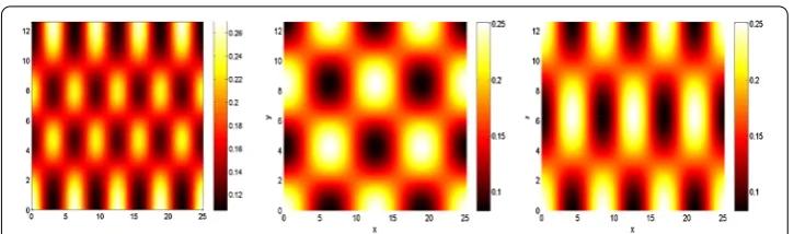
Figure 6 Subcritical case.In Figure 6, we give the comparison among the numerical solution of system (1.3) (left), the weakly nonlinear first order approximation of the solution (medium) and the weakly nonlinear fifth order approximation of the solution (right) under subcritical case. The parameters are chosen asr1= 0.6,

r2= 0.3,c1=c2= 0.1,d1=d2= 0.01,α12= 0.6,β1= 0.02,α21= 0.3,a1= 0.1,a2= 0.2. Herebc= 0.045,ε= 0.1,

b= 1.0101bc_{= 0.0455.}

Figure 7 Bifurcation diagram of the quintic Stuart-Landau equation (4.24).In Figure 7, the values of the parameters are the same as in Figure 6. Herebs= 0.0444 andbc= 0.045. The solid line indicates the stable states and the dashed line indicates the unstable ones.

Figure  presents a complete bifurcation diagram for the bifurcation parameterb. It also shows that system (.) is a stable stationary pattern with a large amplitude branch which coexists in the rangebs<b<bc, which is known as a hysteresis cycle. Varying the

bifur-cation parameterbfollowing the direction of the arrows in Figure , the corresponding numerical solution of the full system shows the hysteresis phenomenon.

4.2 Double and non-resonant eigenvalue

Whenm= , the two pairs of allowed spatial modes (φ,ψ) and (φ,ψ) satisfy the

fol-lowing no-resonance condition []:

φi+φj=φj or ψi–ψj=ψj

and

φi–φj=φj or ψi+ψj=ψj,

(.)

Pushing weakly nonlinear analysis up toO(ε_{), we get the following Stuart-Landau}

equa-tions for the amplitudesAandAat the timeT(T):

dA

dT =σA–LA



+SAA,

dA

dT =σA–LA



+SAA,

(.)

where the coefficientsσ,Ll,Sl, withl= , , are given in Appendix A... For the existence

and stability of the equilibria of equations (.), we have the following propositions.

Proposition .

(i) The trivial equilibriumE= (, )always exists.

(ii) The boundary equilibriaE±_ = (±σ

L, )exist if and only ifL> .

(iii) The boundary equilibriaE±_ = (,±_Lσ

)exist if and only ifL> .

(iv) The interior equilibriaE±_ = (±

σ(L+S) LL–SS,±

σ(L+S)

LL–SS)exist if and only if either

LL–SS< ,L+S< ,L+S< orLL–SS> ,L+S> ,L+S> .

By a linear stability analysis, we have the following results.

Proposition .

(i) The trivial equilibriumEis an unstable node.

(ii) The boundary equilibriaE±_ are stable nodes ifL+S< .

(iii) The boundary equilibriaE±_ are stable nodes ifL+S< .

(iv) The interior equilibriaE±_ are locally asymptotically stable ifLL–SS> ,

L+S> ,L+S> andLS+LS+ LL> ,while they are saddle points if

LL–SS< ,L+S< andL+S< .

Proof (i), (ii) and (iii) are easily checked; here we omit their proofs. For (iv), we only give the proof for the positive equilibriumE_+= (

σ(L+S) LL–SS,

σ(L+S)

LL–SS) as the other cases can be

proved similarly. Linearizing system (.) aboutE+_yields the Jacobian matrix as follows:

J= ⎛ ⎜ ⎝

–σLL–σLS

LL–SS S

σ(L+S) LL–SS

σ(L+S) LL–SS

S

σ(L+S) LL–SS

σ(L+S) LL–SS

–σLL–σLS LL–SS

⎞ ⎟ ⎠.

Then the characteristic equation of the linearized system can be calculated as follows:

λ+σ(LS+LS+ LL) LL–SS

λ+σ

_(L

+S)(L+S)

LL–SS

= . (.)

WhenLL–SS> ,L+S> ,L+S>  andLS+LS+ LL> , it is easy to know

that all the zeros of the characteristic equation (.) have negative real parts. However, the characteristic equation (.) has at least one positive real zero whenLL–SS< ,

L+S<  andL+S< . This completes the proof.

Figure 8 Single mode pattern.Figure 8 gives the comparison among the numerical solution of system (1.3) (left), the weakly nonlinear first order approximation of the solution with stable equilibrium (A1∞, 0) (medium) and the weakly nonlinear first order approximation of the solution with stable equilibrium (0,A2∞) (right) under double and non-resonant eigenvalue case. The parameters arer1= 0.6,r2= 0.3,c1=c2= 0.1,

d1=d2= 0.1,α21= 0.3,a1= 0.1,a2= 0.2,α12= 0.4,β1= 0.2. Herebc= 0.993,ε= 0.36 andb= (1 +2)bc.

equilibriaE,Eis stable, the interior equilibriaE± are all unstable. Thus, we shall

distin-guish two kinds of stationary patterns: (i): a single mode stationary pattern when any of the equilibriaE±_ orE±_ is stable; (ii): a mixed-mode stationary pattern when any of the equilibriaE±_ is stable.

Remark  It should be pointed out that the stability condition of the interior equilibria

E±_ requires thatLS+LS+ LL>  but notLS+LS+ LL< , emerging in [].

Here we give a detailed analysis and the corrected proof.

Suppose that system (.) admits at least one stable equilibrium (A∞,A∞). Then we

have the following conclusion.

Proposition . Assume that the hypothesis(i)of Proposition.and the no-resonance

condition(.)hold.Then system(.)has an asymptotic solution,

u(x,y) v(x,y)

=

u∗

v∗

+ε



i=

Ai∞cos(φix)cos(ψiy) +O

ε , (.)

where(A∞,A∞)is a stable equilibrium of system(.).

In Figure , we show the pattern formation, starting from initial conditions, which re-veals random periodic perturbations about the equilibrium (., .). Here we con-sider the rectangular domain with Lx= π andLy= π. With these parameter values

the only admitted unstable mode is chosen as kˆ

c = .∈[., .], which is

the band of the unstable modes. Then there exist two mode pairs (, ) and (, ) which satisfy the condition (.) and the non-resonant condition (.). By a calculation, we haveL=L= .,S=S= –.. Then we getL+S=L+S= –. < ,

LL–SS= –. < . Therefore, the equilibriaE± andE± are all stable andE± are

all unstable. Therefore, the predicted asymptotic solution is the following single mode pattern:

Figure 9 Mixed-mode pattern.Figure 9 gives the comparison between the numerical solution of system (1.3) (left) and the weakly nonlinear first order approximation of the solution (right) in the double and non-resonant eigenvalue case. The parameters are the same as in Figure 6 except thatα12= 0.5 and

β1= 0.02. Herebc= 0.2676,ε= 0.1 andb= (1 +ε2_)bc_.

Figure 10 Mixed-mode super-squares pattern.Figure 10 gives the comparison between the numerical solution of system (1.3) (left) and the weakly nonlinear first order approximation of the solution (right) under double and non-resonant eigenvalue case. The parameter values are chosen the same as in Figure 9. Here a square domain withLx=Ly= 8πis chosen.

or

w=εA∞cos(.x)cos(.y) +O , (.)

whereA∞andA∞are the coordinates of the equilibriaE± andE±, respectively. In

Fig-ure , we see a good qualitative agreement of the approximation (.) or (.) with the numerical solution of the full system (.).

According to the parameter values of Figure , the only admitted unstable mode is cho-sen as kˆc = ., which belongs to the band of unstable modes allowed by the

bound-ary conditions. Then the two mode pairs (, ) and (, ) satisfy the conditions (.) and (.). From (.), we obtainσ=σ= .,L=L= .,S=S= –.. Thus

the only stable positive equilibrium isE+_according to Proposition .. Therefore, the pre-dicted asymptotic solution given by the positive equilibriumE_+is the following mixed-mode pattern:

w=εA∞cos(x)cos(.y) +A∞cos(.x)cos(y) +O , (.)

whereA∞andA∞are the coordinates of the positive equilibriumE+. Figure  provides

the comparison between the numerical solution of system (.) and the weakly nonlinear approximation solution withLx= πandLy= πat the first order.

According to the parameter values of Figure , the only unstable model is chosen as ˆ

k

two mode pairs (, ) and (, ) satisfying the conditions (.) and (.). The predicted asymptotic solution has the same form as (.). From Figures  and , we see a signifi-cant quantitative discrepancy between the numerical solution of the original system and the approximated solution. The fact that the weakly nonlinear analysis has poorer perfor-mances in predicting the mixed-mode pattern was also reported in [].

4.3 Double and resonant eigenvalue

Whenm= , the two pairs of allowed spatial modes (φ,ψ) and (φ,ψ) satisfy the

fol-lowing resonance condition []:

φi+φj=φj and ψi–ψj=ψj

or

φi–φj=φj and ψi+ψj=ψj,

(.)

withi,j= ,  andi=j. In what follows, without of loss generality, we shall assume that the first conditions in (.) hold withi= ,j= . Thus it follows thatφ= ,ψ=kˆc,ψ=kˆ_c,

φ=

√

ψandψ= ψ.

When the resonance condition (.) holds, the solution (.) at the orderεreads

w=Acos(

√

ψx)cos(ψy) +Acos(ψy). (.)

By imposing the solvability condition atO(ε) to equation (.), we obtain the Stuart-Landau equations as follows:

∂A

∂T

=σA˜ –LA˜ A,

∂A

∂T

=σ˜A–

˜ L A

 .

(.)

Here the coefficientsσ˜ andL˜are given in Appendix A...

It is easy to see that the steady states of equation (.) are the trivial equilibrium (, ) andE±= (±_L˜σ˜,σ_L˜_˜). By computing the eigenvalues of the Jacobian matrix evaluated atE±, we obtain the stationary solutionsE±are always unstable, and it is not possible to pre-dict the amplitude of the pattern at this order. Therefore the weakly nonlinear analysis as regards the amplitude has to be pushed to a higher order to obtain some qualitatively results. Pushing the weakly nonlinear analysis toO(ε_{), we obtain the following}

Stuart-Landau equations for the amplitudesAandAat the timeT(T,T):

dA

dT =σ¯A–L¯AA+γ¯A



+δ¯AA,

dA

dT =σ¯A–L¯A



+γ¯A+δ¯AA,

(.)